Article

A New Approach to Approximate Solutions of Single Time-Delayed Stochastic Integral Equations via Orthogonal Functions

1
Department of Mathematics, Karaj Branch, Islamic Azad University, Karaj 31499-68111, Iran
2
LAETA/INEGI, Faculty of Engineering, University of Porto, 4200-465 Porto, Portugal
*
Author to whom correspondence should be addressed.
Symmetry 2022, 14(10), 2085; https://doi.org/10.3390/sym14102085
Submission received: 3 September 2022 / Revised: 29 September 2022 / Accepted: 1 October 2022 / Published: 7 October 2022
(This article belongs to the Special Issue Differential/Difference Equations and Its Application)

Abstract

:
This paper proposes a new numerical method for solving single time-delayed stochastic differential equations via orthogonal functions. The basic principles of the technique are presented. The new method is applied to approximate two kinds of stochastic differential equations with additive and multiplicative noise. Excellence computational burden is achieved along with a O ( h 2 ) convergence rate, which is better than former methods. Two examples are examined to illustrate the validity and efficiency of the new technique.

1. Introduction

Many real-world problems are mathematically formulated in terms of differential equations (DEs), integro-differential equations (IDEs) or partial differential equations (PDEs). Symmetry plays an important role in the study of many types of these equations [1,2,3]. Stochastic differential equations (SDEs) are often adopted to model the time evolution of systems in the areas of biology, physics, economics, and engineering, among others. SDEs have an important role in explaining some symmetry phenomena, namely symmetry breaking in molecular vibration [4]. Due to physical constraints, it is often necessary to introduce time delays into the equations in order to take into account the fact that systems’ response to inputs or perturbations is not instantaneous, leading to the so-called stochastic delayed differential equations (SDDEs). Indeed, energy transfer or signal transmission might be the origin of delay terms. Recurrently, the calculation of the reaction of time-delay systems turns out to be incredibly demanding. However, regardless of the challenges, addressing such issues ends up being unavoidable.
Solving SDDEs is an open issue, and different numerical methods have been proposed. Among them, orthogonal functions can reduce the SDDEs to a linear system of algebraic equations, whose solution describes approximately the behavior of the original system.
In the follow-up, we consider:
j ( ζ ) = j 0 ( ζ ) + 0 ζ k 1 s , ζ · j ( s τ ) d s + 0 ζ k 2 s , ζ · j ( s τ ) d W ( s ) , ζ 0 , ζ , j ( ζ ) = μ ( ζ ) , ζ τ , 0 ,
where j ( ζ ) , j 0 ( ζ ) , k 1 ( s , ζ ) , k 2 ( s , ζ ) , and the 1-D Wiener process W ( ζ ) , for s , ζ [ 0 , Z ) , are stochastic processes defined on the same probability space ( Ω , ϝ , P ) , with a filtration F ζ . These satisfy the usual conditions, namely: (i) right-continuous filtration F ζ ζ 0 ; (ii) each F ζ , ζ 0 contains all P-null sets in F; and (iii) j ( ζ ) is an unknown function, and 0 ζ k 2 ( s , ζ ) · j ( s τ ) d W ( s ) is a stochastic integral that is interpreted in the Itô sense [5].
We are interested in the response to the initial function j ( ζ ) = μ ( ζ ) or the parameters contained in the SDDEs. In fact, extra data are required to deal with a system of delayed differential equations (DDEs). Since the derivative of Equation (1) depends upon the solution at former time ζ τ , it is essential to give an initial history function to determine the value of the solution before time ζ = 0 . In many usual models, the history is a constant vector. However, non-constant history functions are experienced regularly. The initial time is a jump derivative discontinuity in most problems. Moreover, any solution or derivative discontinuity in the history function at preceding points to the initial time should be dealt with suitably since such discontinuities can spread to after-times.
Numerical analysis of SDDEs based on the Euler–Maruyama scheme was suggested by Buckwar [6]. Triangular functions (TFs) were proposed for the analysis of dynamic systems by Deb et al. [7]. Numerical and computational methods for solving SDEs based on TF and block pulse function (BPF) methods were presented by Khodabin et al. [8]. Operational matrices of BPFs for Taylor series and Bernstein polynomials were computed by Marzban et al. [9] and by Behroozifar et al. [10].
In this paper, we will be keen on obtaining SDDEs approximations via the TFs method. The new approach leads to O ( h 2 ) convergence rate, which is better than alternative methods [11]. The rest of the paper is organized as follows. In Section 2, the basics of TFs and operational delayed matrices are introduced. In Section 3, the new method is presented. In Section 4, two numerical examples are studied. In Section 5, the main conclusion remarks are given.

2. Basic Concepts of Triangular Functions

The TFs originate from a simple dissection of BPFs, where ϕ i ( ζ ) = T i 1 ( ζ ) + T i 2 ( ζ ) is the i-th BPF such that:
T i 1 ζ = 1 ζ i h h i h ζ < ( i + 1 ) h , 0 otherwise . T i 2 ζ = ζ i h h , i h ζ < ( i + 1 ) h , 0 otherwise ,
where h = Z m with Z = 1 is considered herein in the interval ζ [ 0 , Z ) . Therefore, some basic properties, such as orthogonality, finiteness, disjointedness and orthonormality are shared by both.
Two m-set TF vectors are defined in [ 0 , Z ) as T 1 ( ζ ) = T 0 1 ( ζ ) , T 1 1 ( ζ ) , , T m 1 1 ( ζ ) T , T 2 ( ζ ) = T 0 2 ( ζ ) , T 1 2 ( ζ ) , , T m 1 2 ( ζ ) T , and the 1-D TF vector is:
T ( ζ ) = T i 1 ( ζ ) , T i 2 ( ζ ) T ,
where T denotes transposition for i = 0 , 1 , , m 1 . From the above representation, it follows that:
T ( ζ ) · T T ( ζ ) = diag ( T ( ζ ) ) = T ^ ( ζ ) , T ( ζ ) · T T ( ζ ) · J J ˜ · T ( ζ ) , T T ( ζ ) · B · T ( ζ ) B · T ( ζ ) ,
such that T ^ ( ζ ) is a 2 m × 2 m diagonal matrix, and B is a 2m-vector with elements equal to the diagonal entries of matrix B. Moreover,
0 ζ T i p s · T j q s d s = δ i j × h 3 p = q 1 , 2 , h 6 p q .
There are some details that make the TF-based methods more efficient than others. Indeed, determining the coefficient vectors of j0(ζ) in the TF method needs only samples instead of the usual integration and scaling. Another option is a TF piece-wise linear solution, which in most cases leads to a smaller error than the staircase solution of the BPF piece-wise constant. A square integrable function j0(ζ) over [0, Z) can be broadened into an m-set TF series as:
j ζ j ^ ( ζ ) i = 0 m 1 J i 1 · T i 1 ζ + i = 0 m 1 J i 2 · T i 2 ζ = J 1 J 2 T 1 ζ , T 2 ζ = J T · T ζ 2 m × 2 m ζ 0 , Z ,
where J i 1 = j ( i · h ) and J i 2 = j ( i + 1 · h ) for i = 0 , 1 , , m 1 , and J 1 , J 2 are coefficient vectors. The operational matrix for integration of TFs, for i = 0 , 1 , , m 1 , is derived as upper triangular matrices:
0 ζ T s d s = 0 ζ T 1 s d s 0 ζ T 2 s d s = P 1 · T 1 ζ + P 2 · T 2 ζ P 1 · T 1 ζ + P 2 · T 2 ζ = P · T ( ζ ) ,
where
P = P 1 P 2 P 1 P 2
and
P 1 = h 2 0 1 1 1 0 0 1 1 0 0 0 1 0 0 0 0 m × m P 2 = h 2 1 1 1 1 0 1 1 1 0 0 1 1 0 0 0 1 m × m ,
with
0 ζ T s · d W s P S · T ζ ,
where
P S = P S 1 P S 1 P S 2 P S 2 ,
P S 1 = α 0 β 0 β 0 β 0 0 α 1 β 1 β 1 0 0 α 2 β 2 0 0 0 β m 2 0 0 0 α m 1 m × m ,
P S 2 = γ 0 ρ 0 ρ 0 ρ 0 0 γ 1 ρ 1 ρ 1 0 0 γ 2 ρ 2 0 0 0 ρ m 2 0 0 0 γ m 1 m × m , α i : = i + 1 W i + 0.5 h W ( i h ) 1 h i · h i + 0.5 h s d W ( s ) , β i : = i + 1 W i + 1 · h W ( i · h ) 1 h i · h i + 1 h s d W ( s ) , γ i : = i W i + 0.5 h W ( i h ) 1 h i h i + 0.5 h s d W ( s ) , ρ i : = i W i + 1 · h W ( i · h ) 1 h i · h i + 1 · h s d W ( s ) .
A function of two variables k s , ζ can be expanded with respect to TFs as k s , ζ = T T ( ζ ) K T ( s ) , where T ( s ) and T ( ζ ) are 2 m 1 D and 2 m 2 D triangular vectors, and K is a 2 m 1 × 2 m 2 coefficient matrix of TFs. For simplicity, we put m 1 = m 2 = m . Therefore, K can be written as:
K = K 11 m × m K 12 m × m K 21 m × m K 22 m × m 2 m × 2 m ,
where K 11 , K 12 , K 21 , K 22 can be computed by sampling k s , ζ at points s i and ζ i such that s i = t i = i · h for i = 0 , 1 , , m 1 . Therefore, the following approximations can be obtained:
K 11 i , j = k s i , ζ j i , j = 0 , 1 , , m 1 , K 12 i , j = k s i , ζ j i = 0 , 1 , , m 1 , j = 1 , , m , K 21 i , j = k s i , ζ j i = 1 , , m j = 0 , 1 , , m 1 , K 22 i , j = k s i , ζ j i , j = 1 , , m ,
and
k l ( s i , ζ j ) = 1 h 2 ( i 1 ) · h i h ( j 1 ) h j h k l ( s , ζ ) d ζ d s , l = 1 , 2 .
As noticed in [12],
j 0 ( ζ τ ) j 0 T · T ( ζ τ ) = j 0 T × T 1 ( ζ τ ) T 2 ( ζ τ ) ,
where J 0 T = J 0 1 , J 0 2 , , J 0 m is the coefficient vector defined as:
J 0 i = 1 h ( i 1 ) · h i h j 0 ζ τ d ζ .
The delay function T ( ζ τ ) in (3) is the transfer of T ( ζ ) defined in (1) over the time axis by ( τ ) . The general definition is given by:
T ( ζ τ ) = T 1 ( ζ τ ) T 2 ( ζ τ ) 2 m × 1 = Q m × m · T 1 ( ζ ) Q m × m · T 2 ( ζ ) 2 m × 1 = Q 2 m × 2 m · T 1 ( ζ ) T 2 ( ζ ) 2 m × 1 , ζ > τ
where Q 2 m × 2 m is defined as the Kronecker delta:
Q 2 m × 2 m = I l Q m × m = Q m × m 0 ¯ 0 ¯ Q m × m 2 m × 2 m i = 1 , 2 , , l ,
where I l is the l-D identity matrix, and ⊗ denotes the Kronecker product [13], while Q is the delay operational matrix of the TF domain. We can derive the delay matrix as follows:
T i 1 ( ζ τ ) = T i 1 ( ζ k h ) , k = 1 , 2 , , m 1 , = 1 i 1 Z m ζ k h < i Z m , 0 elsewhere , = 1 i + k 1 Z m ζ < i + k Z m , 0 elsewhere , = T i + k 1 ( ζ ) .
Thus, one has:
Q = 0 0 k × 1 1 0 0 0 0 1 0 0 0 0 1 0 0 0 0 1 k × k 0 1 × 1 0 0 1 × k m × m .

3. Problem Statement

Many systems are impacted by positive and negative feedback. Such mechanisms push the system to a new state of equilibrium or back to its primary state [14].
Consider a simple delayed feedback by j ( ζ ) = α · j ( ζ τ ) , where α is a real value and τ 0 . The cases α > 0 and α < 0 correspond to negative and positive feedback, respectively.
When τ = 0 , we recover a simple ODE. We prescribe j ( ζ ) for τ ζ < 0 as initial data for the upper DE. If such an ODE involves a Gaussian white noise process ξ ( ζ ) = d W ( ζ ) d ζ , then there will be two states, with additive noise α + b ξ ( ζ ) and multiplicative noise j ( ζ τ ) + b · ξ ( ζ ) , in which b is the noise intensity. For further details, please see [15].

3.1. Solving SDDEs Based on Triangular Function Operational Matrices with Additive Noise

Below, we consider a linear stochastic Volterra integral equation with single time delay and intend to obtain the j t coefficient based upon a TF in the interval ζ 0 , Z :
j ( ζ ) = j 0 ( ζ ) + 0 ζ k 1 ( s , ζ ) · j ( s τ ) d s + 0 t k 2 ( s , ζ ) d W ( s ) , τ 0 , Z ) , j ( 0 ) = j 0 , j ( ζ ) = μ ζ , τ ζ < 0 ,
where j 0 is a constant specified vector, k 1 ( s , ζ ) and k 2 ( s , ζ ) are known matrices, and μ ζ is an arbitrary, initial-history-known function. We approximate the j ζ , j 0 ζ , k 1 ( s , ζ ) and k 2 ( s , ζ ) functions by TFs as mentioned below from (6)–(9):
j ( ζ ) T T ( ζ ) · J = J T · T ( ζ ) ,
j 0 ( ζ ) T T ( ζ ) · J 0 = J 0 T · T ( ζ ) ,
k 1 ( s , ζ ) T T ( ζ ) · K 1 · T ( s ) , k 2 ( s , ζ ) T T ( ζ ) · K 2 · T ( s ) ,
j ( ζ τ ) = μ ( ζ τ ) , τ ζ τ < 0 , J T · T ( ζ τ ) = T T ( ζ τ ) · J , 0 ζ τ < T τ ,
where the vectors J , J 0 and matrices K 1 , K 2 are TF coefficients of j ζ , j 0 ζ , k 1 ( s , ζ ) and k 2 ( s , ζ ) , respectively. Replacing the above approximations into (5), we arrive at:
T T ( ζ ) · J T T ( ζ ) · J 0 + 0 τ T T ( ζ ) · K 1 · T ( s ) · μ ( s τ ) d s + τ ζ T T ( ζ ) · K 1 · T ( s ) · T T ( s τ ) · J d s + 0 ζ T T ( ζ ) · K 2 · T ( s ) d W ( s ) ,
where
T T ( s τ ) = Q · T ( s ) ) T = T T ( s ) · Q T ,
where Q 2 m × 2 m is defined as the Kronecker delta (p. 5), and
T T ( ζ ) · J T T ( ζ ) · J 0 + T T ( ζ ) · K 1 0 τ T ( s ) · μ ( ζ τ ) d s + T T ( ζ ) · K 1 · τ ζ T ( s ) · T T ( s ) · Q ^ T · J d s + T T ( ζ ) · K 2 0 ζ T ( s ) d W ( s ) .
Using previous relations:
T T ( ζ ) · J T T ( ζ ) · J 0 + T T ( ζ ) · K 1 · I 1 + T T ( ζ ) · K 1 · τ ζ Z ˜ · T ( s ) d s + T T ( ζ ) · K 2 · I 2 ,
where Z ˜ = diag ( Q T · J ) is a 2m × 2m diagonal matrix. Notice that
I 1 = 0 τ T s μ ( s τ ) d s = 0 τ T 1 s · μ ( s τ ) d s 0 τ T 2 s · μ ( s τ ) d s = 0 τ 1 + i s h · μ ( s τ ) d s 0 τ s h i · μ ( s τ ) d s = 1 + i 0 τ μ ( s τ ) d s 1 h 0 τ s · μ ( s τ ) d s 1 h 0 τ s · μ ( s τ ) d s i 0 τ μ ( s τ ) d s ,
and
I 2 = 0 τ T s · μ ( s τ ) d W ( s ) = 0 τ T 1 s · μ ( s τ ) d W ( s ) 0 τ T 2 s · μ ( s τ ) d W ( s ) = 0 τ ( 1 + i ) s h · μ ( s τ ) d W ( s ) 0 τ s h i · μ ( s τ ) d W ( s ) = ( 1 + i ) 0 τ μ ( s τ ) d W ( s ) 1 h 0 τ s · μ ( s τ ) d W ( s ) 1 h 0 τ s · μ ( s τ ) d W ( s ) i 0 τ μ ( s τ ) d W ( s ) .
Then,
T T ( ζ ) · J T T ( ζ ) · J 0 + T T ( ζ ) · K 1 · I 1 + T T ( ζ ) · K 1 · Q T · J · P · T T ( ζ ) · K 2 · I 2 ,
in which K 1 · Q T · J · P are 2m × 2m matrices, and
T T ( ζ ) · K 1 · Z ˜ · P · T ( ζ ) = B T · T ( ζ ) = T T ( ζ ) · B ,
where B is a 2m-D vector with components equal to the diagonal entries of the matrix K 1 · Q T · J · P , B can be written as B = Π · J and Π = K 1 · P T · Q T . Finally, we arrive at:
T T ( ζ ) · J T T ( ζ ) · J 0 + T T ( ζ ) · K 1 · I 1 + T T ( ζ ) · Π · J + T T ( ζ ) · K 2 · I 2 .
By multiplying both sides in T(ζ) and replacing ≃ with =, we have:
I Π · J J 0 + K 1 · I 1 + K 2 · I 2 ,
which we denote by J00 = J0 + K1 · I1 + K2 · I2, R = I − Π. The solution J is obtained by solving the algebraic equation:
R · J = J 00 .

3.2. Solving SDDEs Based on Triangular Function Operational Matrices with Multiplicative Noise

In the following linear stochastic Volterra integral equations (SVIEs) with single time delay, our purpose is to obtain the TF coefficients of j(ζ) in the interval ζ [ 0 , Z ) :
j ( ζ ) = j 0 ( ζ ) + 0 ζ k 1 ( s , ζ ) · j ( s τ ) d s + 0 ζ k 2 ( s , ζ ) · j ( s τ ) d W ( s ) , τ 0 , Z ) , j ( 0 ) = j 0 , j ( ζ ) = μ ζ , τ ζ < 0 .
Substituting function approximations (6)–(9) into (11), we arrive at:
T T ( ζ ) · J T T ( ζ ) · J 0 + 0 τ T T ( ζ ) · K 1 · T ( s ) · J ( s τ ) d s + τ ζ T T ( ζ ) · K 1 · T ( s ) · T T ( s τ ) · J d s + 0 τ T T ( ζ ) · K 2 · T ( s ) · J ( s τ ) d W ( s ) + τ ζ T T ( ζ ) · K 2 · T ( s ) · T T ( s τ ) · J d W ( s ) ,
and
T T ( ζ ) · J T T ( ζ ) · J 0 + T T ( ζ ) · K 1 · 0 τ T ( s ) · μ ( ζ τ ) d s + T T ( ζ ) · K 1 · τ ζ T ( s ) · T T ( s ) Q ^ T · J d s + T T ( ζ ) · K 2 · 0 τ T ( s ) · μ ( ζ τ ) d W ( s ) + T T ( ζ ) · K 2 · τ ζ T ( s ) · T T ( s ) · Q ^ T · J d W ( s ) ·
Therefore,
T T ( ζ ) · J T T ( ζ ) · J 0 + T T ( ζ ) · K 1 · I 1 + T T ( ζ ) · K 1 · Z ˜ · τ ζ T ( s ) d s + T T ( ζ ) · K 2 · I 2 + T T ( ζ ) · K 2 · Z ˜ · τ ζ T ( s ) d W ( s ) ,
where I 1 , I 2 and both integrals are as considered in the previous section. Then,
T T ( ζ ) · J T T ( ζ ) · J 0 + T T ( ζ ) · K 1 · I 1 + T T ( ζ ) · K 1 · Q ^ T · J · P · T ( ζ ) + T T ( ζ ) · K 2 · I 2 + T T ( ζ ) · K 2 · Q ^ T · J · P S · T ( ζ ) .
Thus, Q ^ , Π , Π S are 2 m × 2 m matrices, and
T T ( ζ ) · J T T ( ζ ) · J 0 + T T ( ζ ) · K 1 · I 1 + T T ( ζ ) · Π · J + T T ( ζ ) · K 2 · I 2 + T T ( ζ ) · Π S · J ,
in which
B 1 = K 1 · P T · Z ˜ T = K 1 · P T · Q ^ T J = Π · J Π = K 1 · P T · Q ^ T , B 2 = K 2 · P S T · Z ˜ T = K 2 · P S T · Q ^ T J = Π S · J Π S = K 2 P S T · Q ^ T .
Lastly, by multiplying both sides in T ( ζ ) , we arrive at:
I Π Π S · J J 0 + K 1 · I 1 + K 2 · I 2 ,
and replacing ≃ with =, we have
R · J = J 00 .
Equations (10) and (12) are linear systems of equations with lower triangular coefficient matrices that give the approximate triangular coefficients of the unknown stochastic processes j ( ζ ) .
This fulfills the assertions.

4. Error Analysis

This part addresses the rate of convergence. The results show a good level of accuracy of order O ( h 2 ) . We utilize Theorem 1 [16] and assert Theorem 2.
Theorem 1
([16]). Suppose that j 0 ζ is an arbitrary real bounded function, which is twice differentiable in the interval 0 , 1 , j ¯ 0 , m ζ correspond to TFs, and j 0 ζ < M for every ζ [ 0 , 1 ] . Then, j ( ζ ) j 0 ( ζ ) < O ( h 2 ) .
Theorem 2.
Let j ζ and j ¯ ζ be solutions of Equations (1) and (6), respectively, and let j ζ < C and k i < C for i = 1 , 2 . Then,
E j ( ζ ) j ¯ ( ζ ) 2 O ( h 2 ) ζ 0 , 1 ,
and
sup 0 ζ < Z E j ζ j ¯ ζ 2 1 2 = O ( h 4 ) ζ 0 , 1 .
Proof. 
We follow with an error analysis in two manners:
  • A: Based on Equation ( 1 ) ,
j ( ζ ) j ¯ ( ζ ) = j 0 ( ζ ) j ¯ 0 ( ζ ) + 0 ζ k 1 ( s , ζ ) · j ( s τ ) d s 0 ζ k ¯ 1 ( s , ζ ) · j ¯ ( s τ ) d s + 0 ζ k 2 ( s , ζ ) d W ( s ) 0 ζ k ¯ 2 ( s , ζ ) d W ( s ) ,
and considering the Euclidean norm:
E j ( ζ ) j ¯ ( ζ ) 2 = E j 0 ( ζ ) j ¯ 0 ( ζ ) + 0 ζ k 1 ( s , ζ ) · j ( s τ ) d s 0 ζ k ¯ 1 ( s , ζ ) · j ¯ ( s τ ) d s + 0 ζ k 2 ( s , ζ ) d W ( s ) 0 ζ k ¯ 2 ( s , ζ ) d W ( s ) 2 ,
and ( a + b + c ) 2 3 ( a 2 + b 2 + c 2 ) , we obtain:
3 E j 0 ( ζ ) j ¯ 0 ( ζ ) 2 + E 0 ζ k 1 ( s , ζ ) · j ( s τ ) d s 0 ζ k ¯ 1 ( s , ζ ) · j ¯ ( s τ ) d s 2 + E 0 ζ k 2 ( s , ζ ) d W ( s ) 0 ζ k ¯ 2 ( s , ζ ) d W ( s ) 2 .
Then, we obtain the last two parts one by one:
I 1 = E 0 ζ k 1 ( s , ζ ) · j ( s τ ) k ¯ 1 ( s , ζ ) · j ¯ ( s τ ) d s 2 = E 0 ζ k 1 ( s , ζ ) · j ( s τ ) k ¯ 1 ( s , ζ ) · j ( s τ ) d s + 0 ζ k ¯ 1 ( s , ζ ) · j ( s τ ) k ¯ 1 ( s , ζ ) · j ¯ ( s τ ) d s 2 2 E 0 ζ k 1 ( s , ζ ) k ¯ 1 ( s , ζ ) · j ( s τ ) d s 2 + 2 E 0 ζ k ¯ 1 ( s , ζ ) · j ( s τ ) j ¯ ( s τ ) d s 2 C 0 ζ E k 1 ( s , ζ ) k ¯ 1 ( s , ζ ) 2 d s + C 0 ζ E j ( s τ ) j ¯ ( s τ ) 2 d s C · O ( h 4 ) + C · O ( h 4 ) = O ( h 4 ) ,
and I 2 = E 0 ζ k 2 ( s , ζ ) k ¯ 2 ( s , ζ ) d W ( s ) 2 = 0 ζ E k 2 ( s , ζ ) k ¯ 2 ( s , ζ ) 2 d s O ( h 4 ) , ( I t o i s o m e t r y ).
Therefore
E j ( ζ ) j ¯ ( ζ ) 2 3 ( O ( h 4 ) + O ( h 4 ) + O ( h 4 ) ) ,
E j ( ζ ) j ¯ ( ζ ) C . O ( h 2 ) .
  • B: Based on Equation (1)
j ( ζ ) j ¯ ( ζ ) = j 0 ( ζ ) j ¯ 0 ( ζ ) + 0 ζ k 1 ( s , ζ ) · z ( s τ ) d s 0 ζ k ¯ 1 ( s , ζ ) · j ¯ ( s τ ) d s + 0 ζ k 2 ( s , ζ ) · j ( s τ ) d W ( s ) 0 ζ k ¯ 2 ( s , ζ ) · j ¯ ( s τ ) d W ( s ) ,
and we obtain the Euclidean norm:
j ( ζ ) j ¯ ( ζ ) 2 = j 0 ( ζ ) j ¯ 0 ( ζ ) 2 + 0 ζ k 1 ( s , ζ ) · j ( s τ ) d s 0 ζ k ¯ 1 ( s , ζ ) · j ¯ ( s τ ) d s 2 + 0 ζ k 2 ( s , ζ ) · j ( s τ ) d W ( s ) 0 ζ k ¯ 2 ( s , ζ ) · j ¯ ( s τ ) d W ( s ) 2
and
E j ( ζ ) j ¯ ( ζ ) 2 3 E j 0 ( ζ ) j ¯ 0 ( ζ ) 2 + E 0 ζ k 1 ( s , ζ ) . j ( s τ ) d s 0 ζ k ¯ 1 ( s , ζ ) . j ( s τ ) d s 2 + E 0 ζ k 2 ( s , ζ ) . j ( s τ ) d W ( s ) 0 ζ k ¯ 2 ( s , ζ ) . j ¯ ( s τ ) d W ( s ) 2 .
By using the Itô isometry property [17] and Theorem 1, we have:
C E j 0 ( ζ ) j ¯ 0 ( ζ ) 2 + 6 0 ζ E k 1 ( s , ζ ) k ¯ 1 ( s , ζ ) · j ( s τ ) 2 d s + 6 0 ζ E k ¯ 1 ( s , ζ ) · ( j ( s τ ) j ¯ ( s τ ) ) 2 d s + 6 0 ζ E k 2 ( s , ζ ) k ¯ 2 ( s , ζ ) · j ( s τ ) 2 d s + 6 0 ζ E k ¯ 2 ( s , ζ ) · ( j ( s τ ) j ¯ ( s τ ) ) 2 d s .
By the problem’s assumption,
C E j 0 ( ζ ) j ¯ 0 ( ζ ) 2 + 6 C 2 0 ζ E k 1 ( s , ζ ) k ¯ 1 ( s , ζ ) 2 d s + 6 C 2 0 ζ E ( j ( s ) j ¯ ( s ) ) 2 d s + 6 C 2 0 ζ E k 2 ( s , ζ ) k ¯ 2 ( s , ζ ) 2 d s + 6 C 2 0 ζ E ( j ( s τ ) j ¯ ( s τ ) ) 2 d s ,
and
E j ( ζ ) j ¯ ( ζ ) 2 O ( h 2 ) ,
We complete the proof.  □

5. Illustrative Examples

Examples are used to demonstrate the theoretical outcomes stated in Section 3 and Section 4. The related computations are performed in M a t l a b ( 2015 a ) .
Let us consider the assumptions:
  • h: h = Z m where Z = 1 in ζ [ 0 , Z ) .
  • ζ i : The number of interval division. t i = i · h node points for i = 0 , 1 , , m .
  • τ : Delay parameter τ = ( k + α ) · h with nonnegative integer α = 0 ( 0 α < 1 ).
  • n: Number of iterations.
  • p: Dividing of interval [ 0 , Z ) in p = m . z equal units. z is a coefficient of m = k . N .
  • σ : Standard deviation.
  • j i : TF coefficient of the analytic solution.
  • j ¯ i : TF coefficient of the approximated method.
  • e: Absolute error computed by e = max 1 i m j i j ¯ i .
  • z ¯ e : Mean of error.
  • s e : Standard deviation of error.
  • U B : Upper bound.
  • L B : Lower bound.
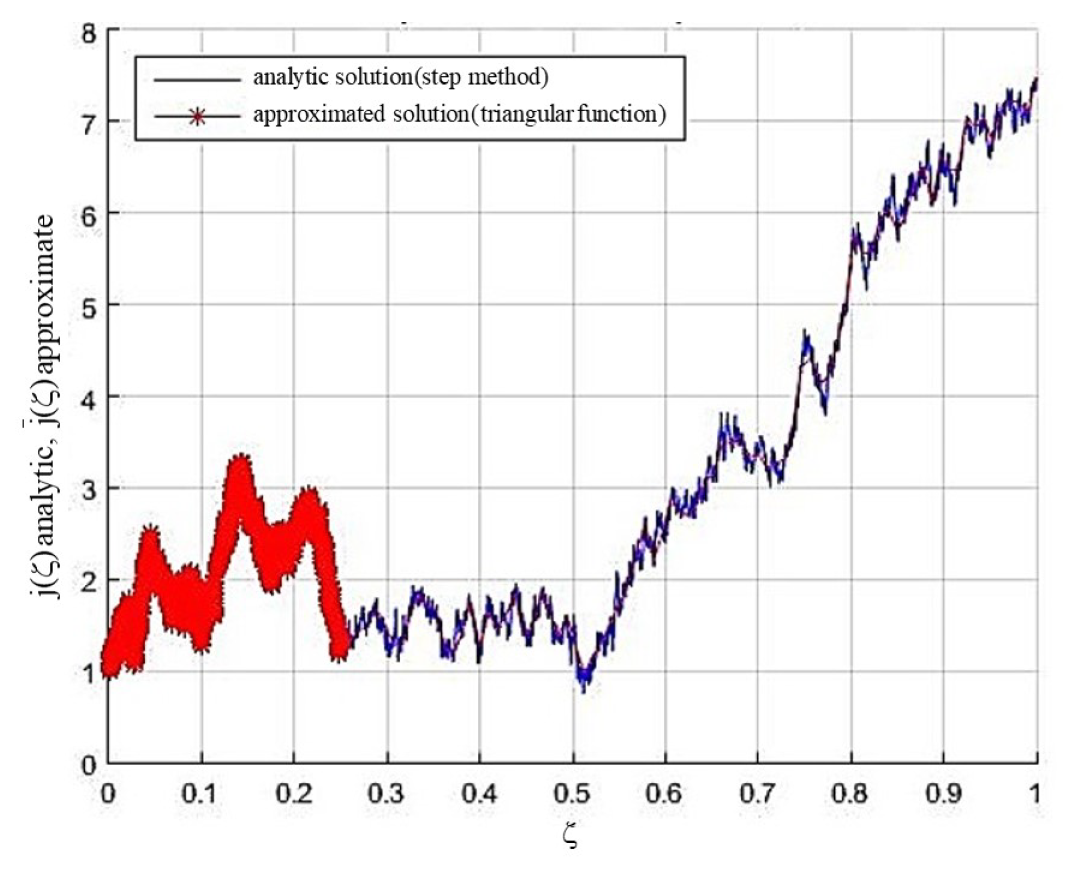
Time delayed equations are mostly solved analytically in a step-wise procedure, called method of steps, with initial condition given [11].
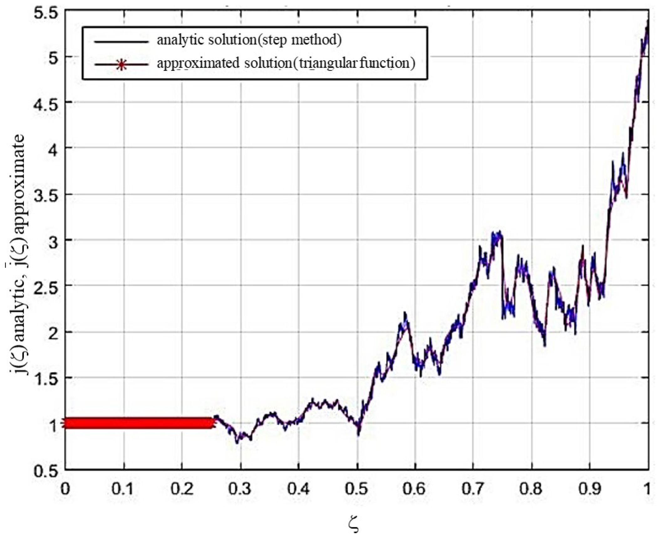
Example 1.
Consider a linear stochastic Volterra integral equation with additive noise input and constant time delay:
j ( ζ ) = j ( 0 ) + 0 ζ 4 j ( s 0.25 ) d s + 4 b 0 ζ d W ( s ) , ζ 0 , 1 , j ( ζ ) = 1 , j ( 0 ) = 1 ,
where j ( ζ ) is an unknown stochastic process on the probability space ( Ω , F , P ) , and W ( ζ ) is a Wiener process:
j ( ζ ) = 1 + 4 b W ( ζ ) , 0 ζ < 1 4 1 + 4 ( ζ 1 4 ) + 4 b 4 1 4 ζ W ( s 1 4 ) d s + W ( ζ ) , 1 4 ζ < 2 4 1 + 4 ζ 1 4 + 8 ( ζ 1 2 ) 2 + 2 4 ζ < 3 4 4 b 16 ( ζ 1 2 ) + 1 4 ζ 1 4 W ( s 1 4 ) d s + 4 1 2 ζ W ( u 1 4 ) d u + 4 1 4 1 2 W ( s 1 4 ) d s + W ( ζ ) , 1 + 4 ζ 1 4 + 8 ( ζ 1 2 ) 2 + 32 3 ( ξ 3 4 ) 3 + 3 4 ζ < 1 4 b 4 3 2 ( ζ 3 4 ) 1 4 ζ 1 2 W ( s 1 4 ) d s + 4 2 ( ζ 3 4 ) 1 2 ζ 1 4 W ( u 1 4 ) d u + W ( ζ ) + 4 3 4 ζ W ( v 1 4 ) d v + 8 ( 1 + 2 ( ζ 3 4 ) ) 1 4 2 4 W ( s 1 4 ) d s + 4 1 2 3 4 W ( u 1 4 ) d u
Example 2.
Assume a linear stochastic Volterra integral equation with multiplicative noise input and time-varying delay as follows:
j ( ζ ) = j ( 0 ) + 0 ζ 4 j ( s 0.25 ) d s + 4 b 0 ζ j ( s 0.25 ) d W ( s ) , ζ 0 , 1 , j ( ζ ) = 1 , ζ 0.25 , 0 , j ( 0 ) = 1 ,
where j ( ζ ) is an unknown stochastic process on the probability space ( Ω , F , P ) , and W ( ζ ) is a Wiener process:
j ( ζ ) = 1 , 0 ζ < 1 4 1 + 4 ( ζ 1 4 ) + b W ( ζ ) W ( 1 4 ) , 1 4 ζ < 2 4 1 + 4 ζ 1 4 + 8 ( ζ 1 2 ) 2 + 4 b 1 2 ζ W ( s 1 4 ) d s 1 2 ζ W ( s ) d s + 2 4 ζ < 3 4 + ζ W ( ζ ) W ( 1 4 ) + b b 1 2 ζ W ( s 1 4 ) d W ( s ) ( 1 + b W ( 1 4 ) ) W ( ζ ) + W ( 1 4 ) ( 1 + b W ( 1 2 ) ) , 1 + 4 ζ 1 4 + 8 ζ 1 2 2 + 32 3 ( ζ 3 4 ) 3 + 3 4 ζ < 1 4 b 3 + b W ( 1 4 ) 3 4 ζ W ( u ) d u b W ( ζ ) W ( 3 4 ) + 4 ( ζ 3 4 ) 1 2 ζ 1 4 W ( s ) d s 1 2 3 4 W ( s ) d s + 3 + b W ( 1 4 ) 3 4 ζ W ( u ) d u 1 2 3 4 W ( s ) d s ( 2 + b W ( 1 4 ) ) 3 4 ζ W ( u 1 4 ) d u + 1 2 3 4 W ( s 1 4 ) d s + 2 ζ 2 W ( ζ ) W ( 1 4 ) + b W ( ζ ) W ( 3 4 ) + 4 ( ζ 3 4 ) 1 2 ζ 1 4 W ( s 1 4 ) d s + b 3 4 ζ u W ( u 1 4 ) d W ( u ) 7 8 W ( 1 4 ) + ζ 2 + b W ( 1 2 ) W ( 1 4 ) 2 + b W ( 1 4 ) W ( ζ ) b W ( ζ ) W ( 3 4 ) + 4 ( ζ 3 4 ) 1 2 ζ 1 4 W ( s ) d s + b 2 b W ( ζ ) W ( 3 4 ) + 4 ( ζ 3 4 ) 1 2 ζ 1 4 W ( s 1 4 ) d W ( s ) + 1 2 3 4 W ( s 1 4 ) d W ( s ) ( 2 + b W ( 1 4 ) ) 3 4 ζ W ( u 1 4 ) d W ( u ) + 2 W ( 1 4 ) + b W ( 1 4 ) W ( 1 2 ) + 7 2 b W ( ζ ) W ( 1 2 ) W ( 1 4 ) 2 + b W ( 3 4 ) .
The numerical results of the mean and standard deviation with 95% confidence intervals for some different values of ζ i in the points h = 1 m are shown in Table 1 and Table 2. Figure 1 and Figure 2 express a trajectory of the approximated solution calculated by the proposed method, along with a trajectory of the analytic solution. It should be noted that due to the high accuracy of the method, in both graphs, the approximated and numerical solutions practically coincide.>

6. Conclusions

In this paper, a new method based on operational matrices of TFs was applied to solve SDDEs with constant time delay. The numerical scheme is computationally simple and revealed good accuracy. An O ( h 2 ) convergence rate is ensured, contrasting with the O ( h ) of other methods. Further research will address numerical solutions to diverse orthogonal functions.

Author Contributions

All authors have contributed to the same extent according to their expertise: S.N.K. in investigation, computer visualization and writing—original draft, M.K. in methodology and the effect of white noise on the solution of delayed stochastic differential equations, R.E. in the conceptualization of the numerical solution of the delayed differential equation, A.M.L. in the investigation of positive and negative feedback systems. All authors have read and agreed to the published version of the manuscript.

Funding

This work was supported by INEGI-LAETA (FCT project UIDB/50022/2020).

Data Availability Statement

Not applicable.

Conflicts of Interest

The authors declare no conflict of interest.

References

  1. Bazighifan, O.; Ali, A.H.; Mofarreh, F.; Raffoul, Y.N. Extended Approach to the Asymptotic Behavior and Symmetric Solutions of Advanced Differential Equations. Symmetry 2022, 14, 686. [Google Scholar] [CrossRef]
  2. Almutairi, A.; Bazighifan, O.; Raffoul, Y.N. Oscillation Results for Nonlinear Higher-Order Differential Equations with Delay Term. Symmetry 2021, 13, 446. [Google Scholar] [CrossRef]
  3. Ma, N.; Wu, Z. Backward doubly stochastic differential equations with Markov chains and a comparison theorem. Symmetry 2020, 12, 1953. [Google Scholar] [CrossRef]
  4. Babaei, A.; Jafari, H.; Banihashemi, S. A collocation approach for solving time-fractional stochastic heat equation driven by an additive noise. Symmetry 2020, 12, 904. [Google Scholar] [CrossRef]
  5. Platen, E.; Bruti-Liberati, N. Numerical Solution of Stochastic Differential Equations with Jumps in Finance; Springer Science & Business Media: Berlin/Heidelberg, Germany, 2010; Volume 64. [Google Scholar]
  6. Buckwar, E. Introduction to the numerical analysis of stochastic delay differential equations. J. Comput. Appl. Math. 2000, 125, 297–307. [Google Scholar] [CrossRef] [Green Version]
  7. Deb, A.; Dasgupta, A.; Sarkar, G. A new set of orthogonal functions and its application to the analysis of dynamic systems. J. Frankl. Inst. 2006, 343, 1–26. [Google Scholar] [CrossRef]
  8. Asgari, M.; Khodabin, M. Computational method based on triangular operational matrices for solving nonlinear stochastic differential equations. Int. J. Nonlinear Anal. Appl. 2017, 8, 169–179. [Google Scholar]
  9. Marzban, H.; Razzaghi, M. Solution of multi-delay systems using hybrid of block-pulse functions and Taylor series. J. Sound Vib. 2006, 292, 954–963. [Google Scholar] [CrossRef]
  10. Behroozifar, M.; Yousefi, S. Numerical solution of delay differential equations via operational matrices of hybrid of block-pulse functions and Bernstein polynomials. Comput. Methods Differ. Equ. 2013, 1, 78–95. [Google Scholar]
  11. Hoseini, S.M.; Marzban, H.R. Analysis of time-varying delay systems via triangular functions. Appl. Math. Comput. 2011, 217, 7432–7441. [Google Scholar] [CrossRef]
  12. Tang, Y.; Li, N.; Liu, M.; Lu, Y.; Wang, W. Identification of fractional-order systems with time delays using block pulse functions. Mech. Syst. Signal Process. 2017, 91, 382–394. [Google Scholar] [CrossRef]
  13. Lancaster, P. Theory of Matrices; Academic Press: New York, NY, USA, 1969. [Google Scholar]
  14. Smith, H.L. An Introduction to Delay Differential Equations with Applications to the Life Sciences; Springer: New York, NY, USA, 2011; Volume 57. [Google Scholar]
  15. Khodabin, M.; Kiaee, N. Stochastic dynamical theta-logistic population growth model. SOP Trans. Stat. Anal. 2014, 1, 3. [Google Scholar] [CrossRef]
  16. Khodabin, M.; Maleknojad, K.; Hossoini Shckarabi, F. Application of triangular functions to numerical solution of stochastic Volterra integral equations. IAENG Int. J. Appl. Math. 2013, 43, 1–9. [Google Scholar]
  17. Klebaner, F.C. Introduction to Stochastic Calculus with Applications; World Scientific Publishing Company: Singapore, 2012. [Google Scholar]
Figure 1. Solving SDDEs (additive noise) via triangular function, n = 40, N = 4, k = 2.
Symmetry 14 02085 g001
Figure 2. Solving SDDEs (multiplicative noise) via triangular function, n = 40, N = 4, k = 2.
Symmetry 14 02085 g002
Table 1. SDDE with additive noise, n = 40, N = 4, k = 2, p = 1040, σ = 0.99, b = 0.85.
ζ i z ¯ e s e LBUB
00000
0.125 0000
0.255 0.00013233 0.013495 0.00039169 0.00012703
0.375 0.00012545 0.012793 0.00037133 0.00012042
0.5 0.00025845 0.026356 0.00076499 0.00024809
0.625 0.00031402 0.032023 0.00092948 0.00030143
0.75 0.00053561 0.054619 0.0015854 0.00051413
0.875 0.0006232 0.063551 0.0018446 0.00059821
1 0.00071978 0.0734 0.0021305 0.00069092
Table 2. SDDE with multiplicative noise, n = 40, N = 4, k = 2, p = 1040, σ = 0.99, b = 0.85.
ζ i z ¯ e s e LBUB
00000
0.125 0000
0.25 0.00011832 0.012066 0.00035023 0.00011358
0.375 0.00015062 0.01536 0.00044583 0.00014459
0.5 0.00017632 0.01798 0.00052188 0.00016925
0.625 0.00026521 0.027044 0.00078498 0.00025457
0.75 0.00019342 0.019724 0.00057251 0.00018567
0.875 0.00026007 0.026521 0.00076978 0.00024964
1 0.00051652 0.052672 0.0015289 0.00049581
Publisher’s Note: MDPI stays neutral with regard to jurisdictional claims in published maps and institutional affiliations.

