1. Introduction
Deep learning has made significant progress in many fields over the past few years. There are multiple types of deep neural networks, including convolutional neural networks (CNNs), recursive neural networks (RNNs), attention-based networks, etc. Among them, attention-based networks have undergone rapid development in recent years, especially transformers, a prominent attention-based network that has achieved significant success in the last two to three years in NLP [
1,
2,
3], computer vision [
4,
5,
6,
7,
8], and other fields.
Inspired by these milestone works, this paper seeks to extend the transformer to the 3D triangle mesh. Point-based transformers [
9,
10,
11,
12] have recently shown excellent performance in point cloud classification, segmentation, and other 3D shape tasks. Although it is a straightforward approach that is directly applied to 3D triangle meshes, point-based transformers are based on 3D Euclidean space and lack information on the topological connections between vertices.
An alternative is to represent a 3D triangle mesh as a graph and use powerful graph-based transformers [
13,
14,
15,
16,
17] to learn the shape. Nevertheless, in addition to the vertex and edge information possessed in graph form, the 3D triangle mesh also contains rich intrinsic manifold properties. Therefore, a vital issue is how to preserve and capture the manifold information on the surface as much as possible while learning the global association map between the input tokens and the global representation of the shape.
This paper presents a novel 3D triangle mesh learning framework named NGD-Transformer to solve the above problem. The proposed method is based on the graph-based transformer, and it aims to keep and capture as much intrinsic manifold information of the 3D mesh as possible. Specifically, this paper combines farthest point sampling (FPS) with the Voronoi segmentation algorithm to generate manifold-preserved, uniform, and non-overlapping mesh patches. However, the vertex number of each patch is not the same. Therefore, for the follow-up processing, self-attention graph pooling (SAG pooling) [
18] is employed for sorting the vertices on each patch and screening out the most representative nodes. These nodes are then reorganized according to their scores to create tokens and raw feature embeddings.
To better exploit the manifold properties of the 3D triangle mesh, we further proposed a novel positional encoding called navigation geodesic distance positional encoding (NGD-PE), which encodes the geodesic distances between vertices in a relative manner. The idea is derived from star-map navigation [
19], in which the global position of an object is determined by the relative distance between the object and the navigation-star sequences. Thus, multiple navigation vertices with uniform and semi-symmetrical distribution on the mesh are generated and used as position references for the remaining vertices. Subsequently, raw feature embeddings and positional encodings are merged as input embeddings and fed to the graph transformer encoder to determine the global representation. The global features are then aggregated by a novel up-pooling operation, which is a structure symmetrical to the graph-pooling operation. The aggregated global features are then fused with the local feature determined from the graph neural networks (GNNs). Based on the subsequent tasks, this paper also designed the classifier and semantic segmentation networks to complete the shape classification and semantic segmentation tasks, respectively.
The main contributions of this paper are as follows.
A novel 3D triangle mesh learning framework, named NGD-Transformer, is proposed. This framework can effectively learn and fuse the local and global information of the mesh.
We propose a token-generation algorithm that combines FPS and Voronoi segmentation to generate manifold-preserved, uniform, and non-overlapping patches and spawn tokens and their representations via SAG pooling.
We further propose a novel geodesic relative positional encoding method called navigation geodesic distance positional encoding (NGD-PE), which encodes the geodesic distance between the vertices relatively for the transformer.
2. Related Works
2.1. Transformer
Transformers first made a breakthrough in NLP and computer vision. We refer the reader to [
1,
2,
3,
4,
5,
6,
7,
8] for detailed information. For transformers applied to 3D shapes, one of the major research topics is the point-based transformers [
9,
10,
11,
12,
20,
21,
22]. The main disadvantage of these methods is that they are based on the 3D Euclidean space, lacking information on the topological connections between vertices. An alternative is to design a transformer based on the 3D triangle mesh manifold space. For example, Sarasua et al. [
23] proposed TransforMesh, which first combined the transformer and mesh for the longitudinal modeling of anatomical meshes. However, handling the edge connection information is problematic for this method. To solve this issue, some researchers process 3D triangle mesh with graph-based transformers. For example, Lin et al. [
24] and He et al. [
25] proposed Mesh Graphormer and GET based on graphs for 3D pose transfer tasks. However, currently, such studies are still rare. One of the reasons for this may be that graph-based transformers are primarily made for general graph structures, while 3D triangle mesh contains rich intrinsic manifold information.
Among the works mentioned above, MeshMAE [
26] is the most relevant study to the proposed method. The main difference between MeshMAE and our proposed model is that we employ the manifold preserved segmentation algorithm to generate uniform and non-overlapping patches without a remeshing operation. In addition, this paper proposes a novel geodesic relative positional encoding method, NGD-PE, for learning geodesic information.
2.2. Mesh Sampling
Currently, mesh sampling is mainly divided into clustering-based [
27,
28] and shape sampling-based [
29,
30,
31,
32] methods. The main drawback of clustering-based approaches is that they destroy the manifold topology of the shape and lead to mesh degeneration. Many scholars use shape-sampling methods to preserve the manifold nature of 3D shapes. For instance, Ranjan et al. [
29] sampled the mesh with the Quadic Error Metrics (QEM) criterion, but it is prone to producing degenerated meshes. Schult et al. [
32] proposed the vertex-clustering method, but it is inclined to non-uniform triangles. Thus, this paper combines the manifold FPS algorithm and the Voronoi segmentation algorithm to generate uniform, non-overlapping, and manifold patches.
2.3. Positional Encoding
A critical step in the transformer is positional encoding, representing the positional interactions between tokens. Currently, it can be divided into two categories: absolute encoding [
3,
7] and relative encoding [
1,
17,
33,
34]. The current 3D mesh transformer mainly uses relative positional encoding based on the graph. For example, Kreuzer et al. [
14] extended spectral encoding to the graph transformer using a pre-computed Laplacian feature vector to add to the raw feature embedding before the input embeddings. Another approach is to use edge weights as relative encodings [
14,
34,
35]. However, the works mentioned above rarely feature the design of positional encodings starting from the 3D manifold surface. In this paper, we present a novel geodesic relative positional encoding method, named NGD-PE, which encodes the geodesic distance between the vertices in a relative manner for the transformer.
3. Preliminary
Generally, a 3D mesh can be expressed as a graph structure , where is the set of vertices, is the set of edges, and is the set of faces. The graph can also be represented by various weight matrices, such as the Euclidean distance matrix, degree matrix, Laplacian matrix, and so on. Vertex feature function is defined by assigning a scalar or vector to the vertex. Given a shape with N vertices, each of which has feature dimension D, the input embedding can then be represented as a matrix . This can be further written as a combination of D vectors, .
A graph neural network can be viewed as nonlinear functional mapping between the graph and the output domain, namely . It can obtain some low-level features (e.g., normal vector, curvature, geodesic distance, etc.) from graph , which can be represented as the vertex feature function , and usually edge list can be represented by an adjacency matrix Thus, in many neural networks, . The output of has multiple situations. For example, if the output of is a category-probability vector, then the neural network is a classification network; if the output of is a class-probability matrix, then the neural network is a segmentation network.
4. Conceptual Framework of the Proposed Method
4.1. Algorithm of the Proposed Method
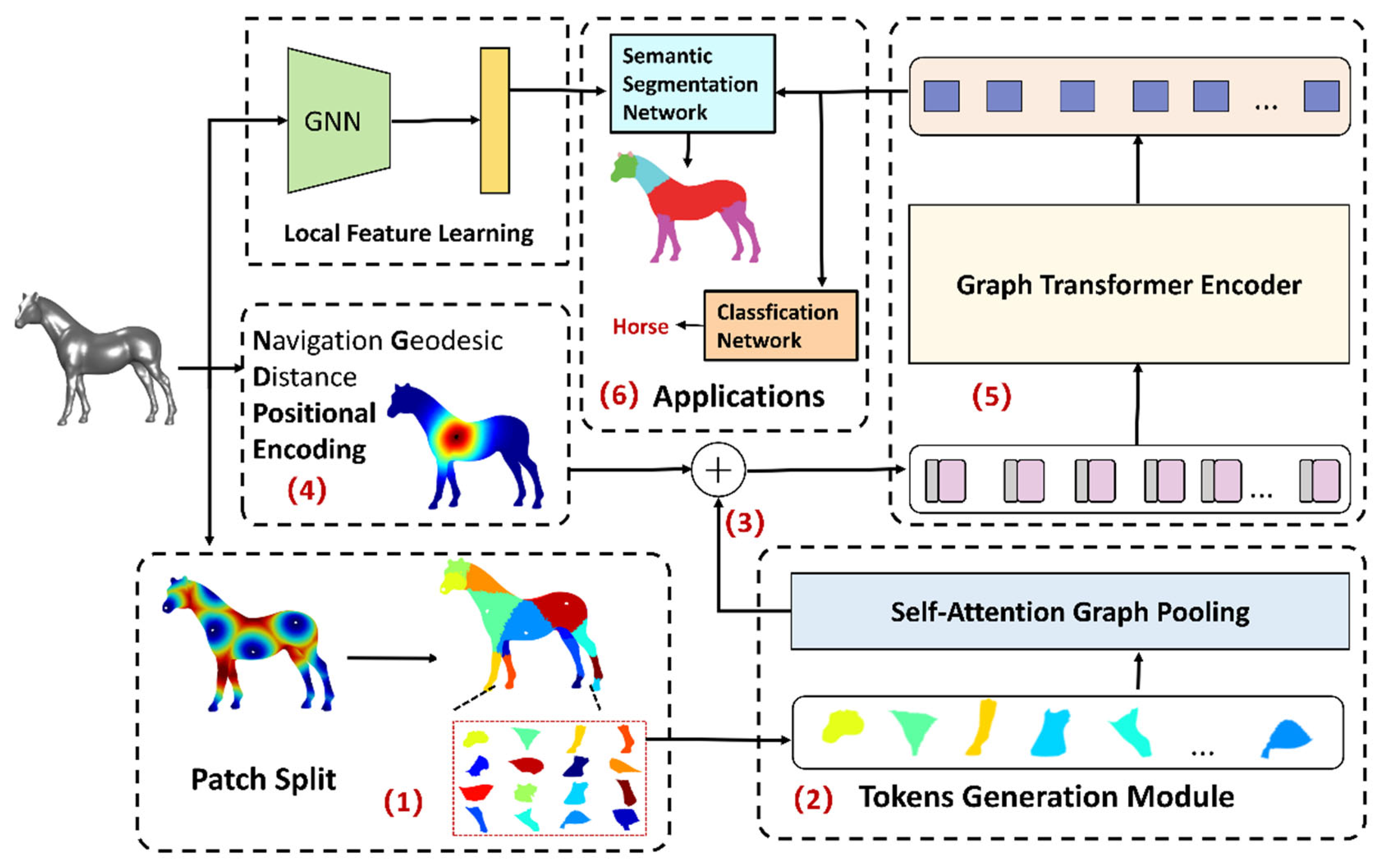
In this section, we introduce the components of our framework. The overall flowchart is shown in
Figure 1. The framework consists of three modules: local feature learning, global representation learning, and application. The global-representation learning module has four parts: patch split, token generation, NGD-PE calculator, and graph transformer encoder. The aim was to change the basic architecture of the graph transformer as little as possible. Therefore, we mainly adapted the transformer and 3D shape in terms of input embedding and positional embedding—specifically, the input embedding format required for the transformer via the patch split and token generation module. The required positional-embedding format was generated by the NGD-PE calculator. Finally, the global association of the above features was determined through the graph transformer encoder. This method also adopted the idea of feature fusion, combining local feature learning with global representation learning to generate richer features.
4.2. Token Generation
In this study, we combined FPS and the Voronoi segmentation algorithm to spawn patches. The proposed method randomly selected a vertex and then used the FPS algorithm to sample a set of uniform seeds on manifold surface, represented as
, and the number of elements is
. After obtaining the initial seeds, each vertex on the surface was labeled using the Voronoi segmentation algorithm. For the
i-th vertex, its patch label is
Here, is the geodesic distance between the i-th vertex and the j-th seed.
In this way, the original model
is divided into
individual non-overlapping patches meeting the following constraint criteria:
where
.
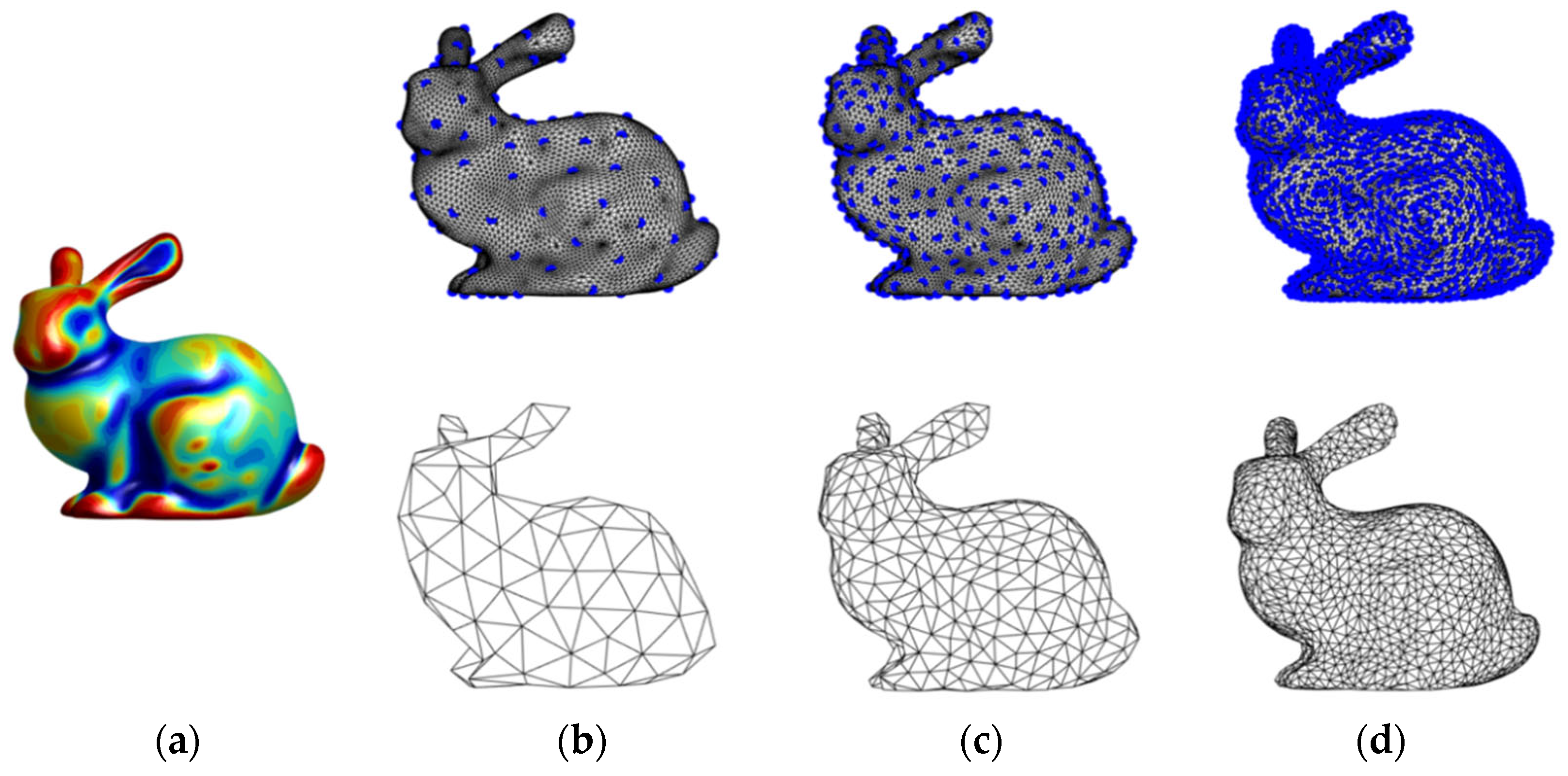
If the vertices in
are triangulated with the Delaunay algorithm, it can be seen that the topology of the whole shape is well preserved. If the number of sampling points is changed, it is able to generate shape representations of different scales (see
Figure 2). Thus, the proposed method split the entire mesh into multiple uniform, manifold-preserved, non-overlapping patches.
Patches can be treated as sub-meshes, but they differ in the number of the vertex. The proposed method selects the most representative nodes in each patch to satisfy the requirements of a unified input embedding shape format. In this method, only the K nodes from each patch are retained using the SAG pooling algorithm. For each patch, the feature of the selected vertices can be denoted as
, and d is the dimension of raw feature embeddings. We further extracted the first top-j vertex in each patch and combined them to form a token sequence
expressed as
, where each row of
represents a token embedding. Furthermore, we further created the K-individual matrices
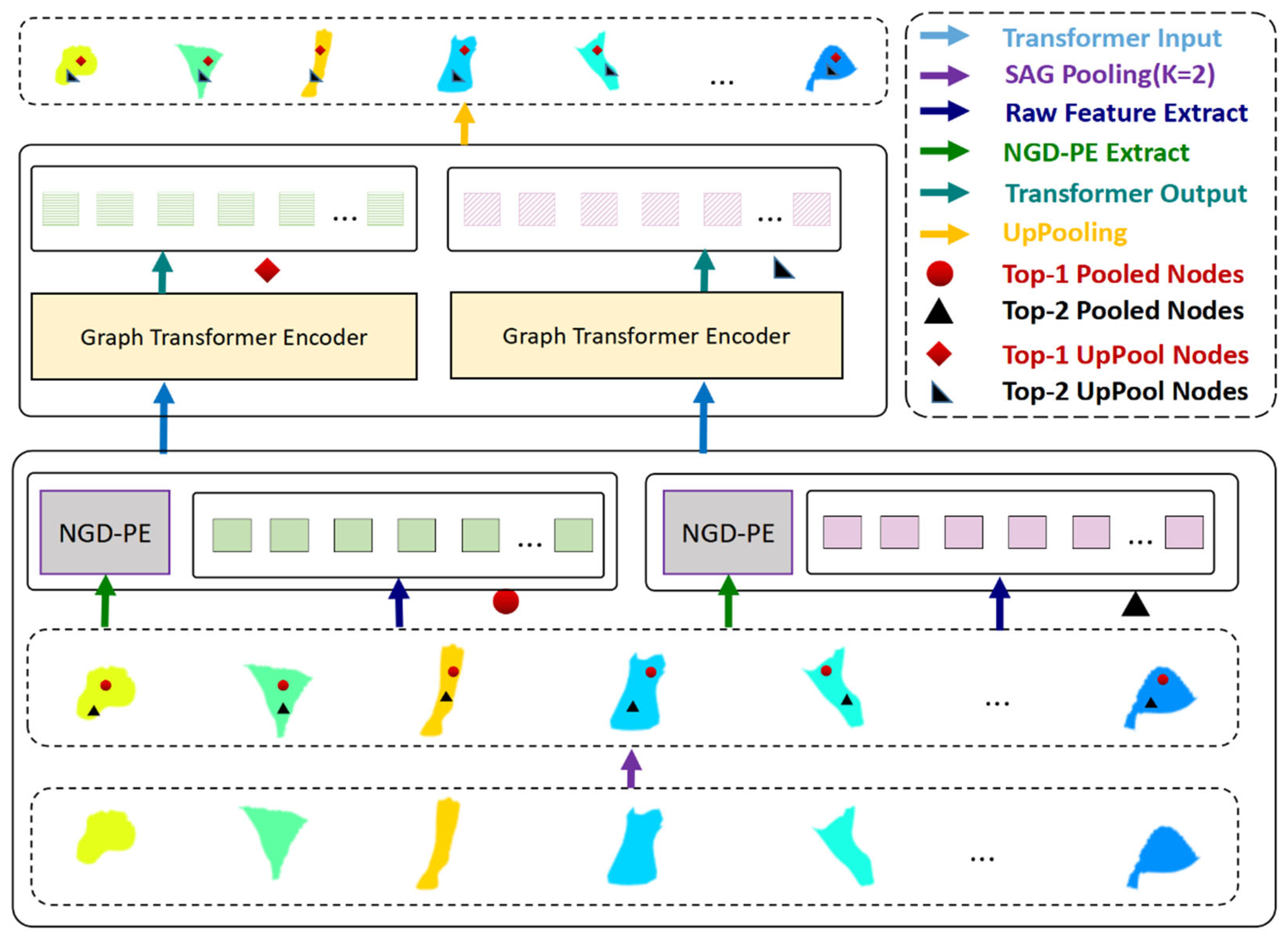
. Subsequently, K graph transformers are designed to learn these K embeddings. Following these few steps, it can directly return the features generated by transformers to the original mesh through pooling indices.
Figure 3 shows the procedure for this part. In this process, the SAG pooling operation and the up-pooling operation are symmetrical in the feature space transformation. In other words, SAG pooling converts graph embeddings to token embeddings, while up-pooling, converts token embeddings to graph embeddings.
4.3. Navigation Geodesic Distance
In measurement theory, a point can be located by at least three non-collinear reference vertices. This principle is widely used in GPS and star map navigation [
19]. It is generally recommended to have uneven and extensive navigation vertices to increase positioning accuracy. It is observed that vertices generated by the FPS satisfy this criterion. Therefore, the FPS algorithm generates a sequence of navigation vertices represented as
, and the number of vertices is
. It can also reuse the vertices in the patch split module or resample the navigation vertices again. The navigational geodesic distance of vertex
i is defined as:
where
is the geodesic distance between the
i-th vertex and the
k-th navigation vertex. The NGD feature distance between the
i-th vertex and the
j-th vertex is further defined via the following formula:
where
> 0,
and
.
Clearly,
satisfies the symmetry property, namely
=
, which guarantees the symmetry of the metric between two nodes. The NGD feature distance also indicates the geodesic proximity of two vertices on a surface. In general, the closer the geodesic distance between vertices, the larger the NGD-feature-distance value. The NGD-feature-distance distribution between a given vertex and the rest of the vertices appears outward-decaying and spatially isotropic and symmetrical (see
Figure 4). The
can control the decay rate of
. Usually, the smaller the value of
, the smaller the decay speed.
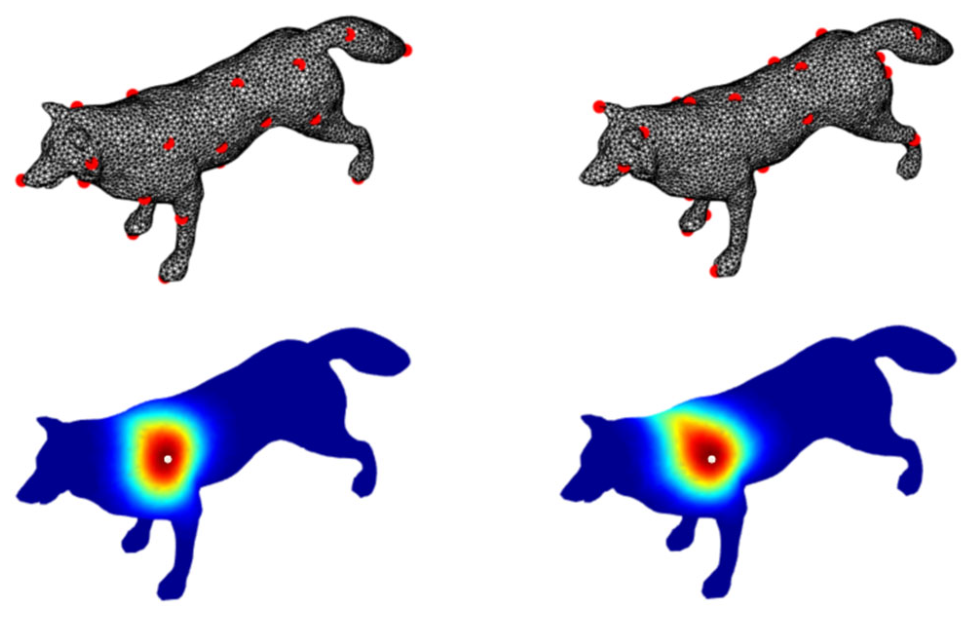
In
Figure 4, the first row represents the navigation vertices gathered through different sampling algorithms. The upper left is the FPS sampling algorithm, the upper right is the random sampling algorithm, and the red vertices are the navigation vertices. The second row describes the navigational geodesic distance of a given vertex
i from the remaining vertices in shape; the red color indicates a larger NGD feature distance, the blue color indicates a smaller NGD feature distance, and the white vertices represent the given vertex i.
The NGD feature distance of each vertex is computed from the set of
to form matrix:
where
.
For the
j-th token in the
l-th token sequence, its global vertex identifier is
, and its input embedding is further generated as follows:
where
and
.
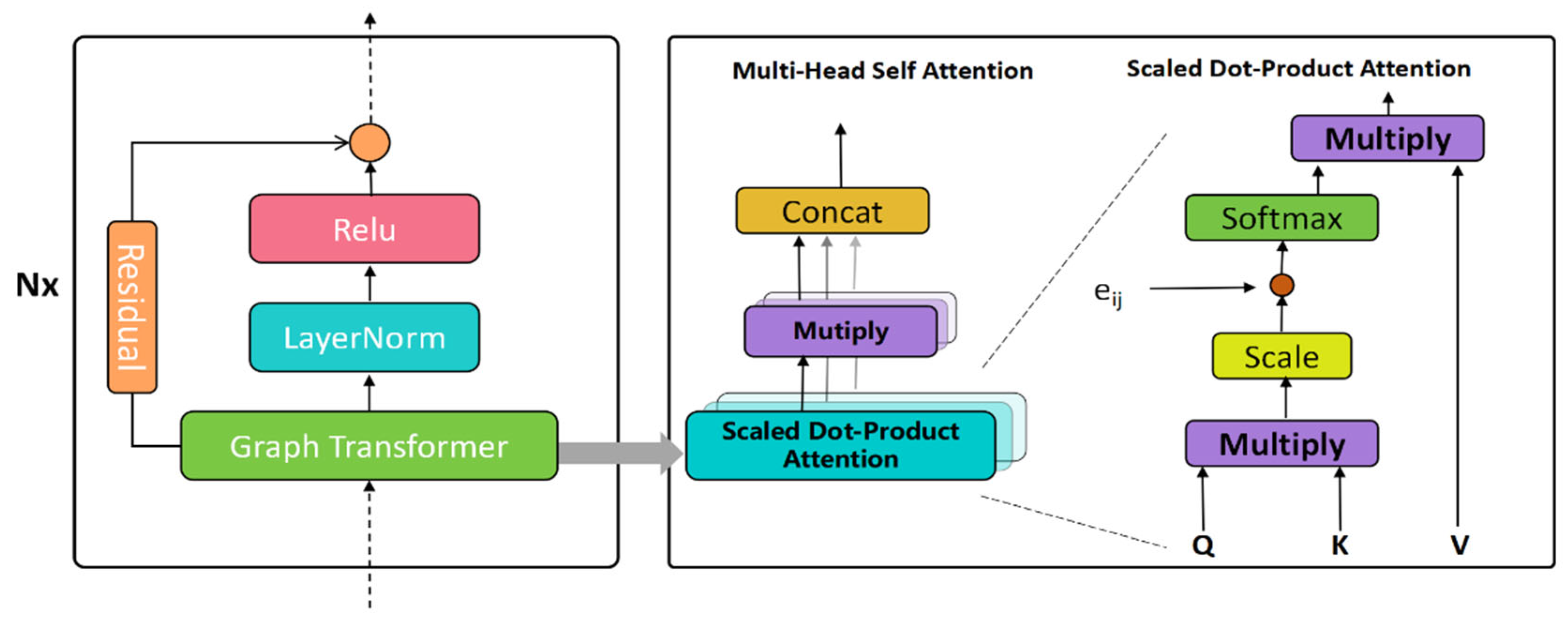
4.4. Graph Transformer Encoder
We adopted the graph transformer frameworks [
15,
17] for learning.
Figure 5 shows the block diagram of our graph transformer encoder. Since
contains the relative position information of the vertex
i and j, it can also be taken as an edge feature. The input embeddings of the
l-th token sequence are
. The multi-head attention coefficients between token
j and token
i are computed as follows:
where
is the exponential scale dot-product function and each head’s hidden size is determined by
d. Following the graph’s multi-head attention, the messages from token
j to source
i are aggregated as follows:
where the || is the concatenation operation for
C head attention.
In the same way as with GAT, it can apply the graph transformer to the last output layer to remove the non-linear transformation by averaging as follows:
We finally stack multiple graph transformer layers to form an encoder module. The output of the graph transformer encoder can be represented as K-individual matrices
,
. For the
j-th token in the
i-th token sequence, the proposed method adopts the pooling indices technology to restore its learned feature to the original mesh as follows:
where
.
4.5. Networks
NGD-Transformer is applied to shape classification and semantic segmentation tasks and design the corresponding network structure for these two tasks.
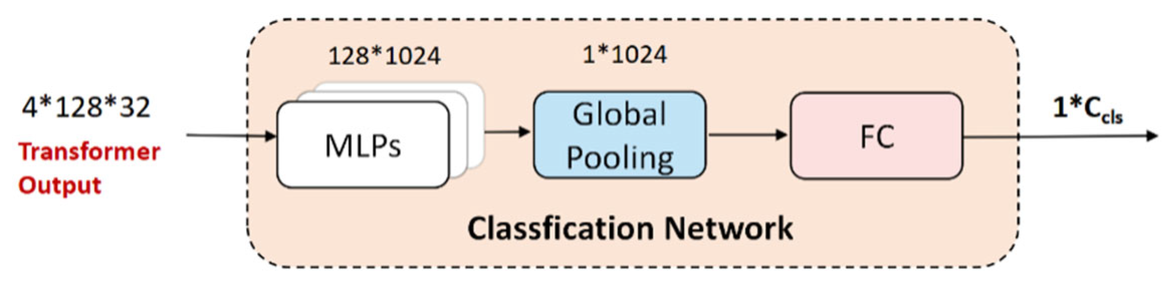
4.5.1. Classification Network
After passing through the transformer module, the embedding representation of the shape is
. It was then reshaped as
. Subsequently, the proposed method performed feature mapping through a set of MLPs and extracted global features through global pooling. Subsequently, the features were further transformed into the target category number via the fully connected network. The network block diagram is shown in
Figure 6.
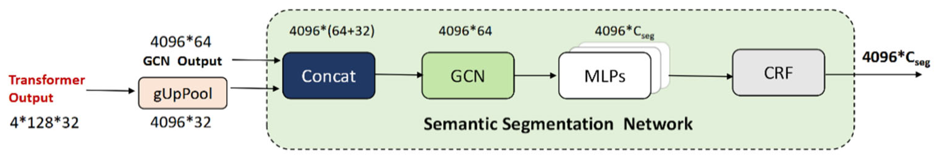
4.5.2. Semantic Segmentation Network
The output embeddings are firstly projected onto the global manifold structure through the up-pooling operation. Next, we combine the mapped features and the local features obtained from the GNN network to generate a new representation of each vertex following feature transformation through a set of MLPs. For the final results, we further post-process and optimize them using the conditional random field (CRF) [
36]. The network block diagram is shown in
Figure 7.
5. Experiments
5.1. Experimental Setting
The PyTorch geometric library was used to implement our method. The networks were trained and tested on a desktop computer with the NVIDIA GeForce RTX 3060 GPU. To increase the training speed, the uniform remeshing algorithm described by Huang et al. [
37] was used to adjust the number of vertices to 2048~8192.
The input features of our network have 38 dimensions with 16 wave kernel signature (WKS) features [
38], 16 spin image (SI) features [
39], 3 coordinate features, and 3 normal vector features, respectively. The above features contained 32 intrinsic features and 6 extrinsic features. These input features were first feature-transformed through a three-layer MLP network.
For the patch split module, the patch number was set between 48 and 96, roughly the square root of the vertex number of 3D mesh. For the NGD-PE calculation module, our navigation number value needed to be consistent with the dimension of the raw feature embeddings. The alpha was set as the default value 1. For the token generation module, the number of vertices, K, was kept with the value ranging from 4 to 16, and the pooling method adopted a graph attention convolution as its GNN network with a multi-head attention head of 2 to 4, which retained enough information without increasing the burden of computation.
For the graph transformer module, we built the association matrix and edge features for any two tokens and used φij as the edge feature. The number of layers of the transformer encoder was set as 3.
We simultaneously used a GNN network, the ChebNet [
40], to learn the local features of the shape. The above is the experimental setting for the public part, and the setting for the application network is explained in detail below.
5.2. Shape Classification Network
In this section, our classifier performance was evaluated. For the classification task, the evaluation was conducted using the ModelNet40 [
41] and ModelNet10. ModelNet40 is a large database of shape classification. It consists of 12,311 CAD models, which are divided into 9840 training models and 2468 testing models. Among them, ModelNet10 contains 4899 CAD models and is a subset of ModelNet40. We manually cleaned this subset of models and aligned their orientations. The shapes were also converted into watertight manifold meshes using the method mentioned in [
37].
Our network structure is shown in
Figure 6. After setting up the public network part, the global pooling was used to obtain the feature representation of the overall shape and then input this feature into a three-layer MLP network. The output of the classifier was the category probability vector. The log_softmax was used as a cost function and implemented the Adam optimizer optimization, with a learning rate of 8 × 10
−4 and a momentum of 0.9. The network was trained in 100 epochs. Finally, the classification accuracy was used as an evaluation indicator.
The results, which are shown in
Table 1, indicated that our method achieves the best results in the dataset MN10. The best results and unreported results for each datasets were labeled in bold font and "-", respectively.
5.3. Shape Semantic Segmentation Network
In this section, we evaluate our semantic segmentation performance. For this task, the evaluation was conducted using the PSB [
45] and COSEG [
46].
According to the Princeton Segmentation Benchmark (PSB), there are 19 categories, each including 20 shapes. Each shape category has 2 to 11 categories.
COSEG has eight scan categories and three synthetic categories, which are mainly used for shape semantic segmentation. The shape numbers varied considerably between the eight scan categories, and there were relatively more models in the three synthetic categories than in the eight scan categories, including Alien (200 meshes) and Vases (300 meshes), and Chairs (400 meshes).
Our semantic segmentation framework is shown in
Figure 7. After the public network had output the global features, the features were then fused with local features into a three-layer MLP network whose output result was the category-probability vector of each vertex. Finally, the results were optimized with CRF. The log_softmax was used as a cost function and implemented the optimization using the Adam optimizer with a learning rate of 8 × 10
−4 and a momentum of 0.92. The network was trained in 50 epochs.
There are many definitions of segmentation accuracy. In this paper, the definition presented by Kalogerakis et al. [
36] was applied, according to which the segmentation accuracy is defined as the ratio of the area of the correctly labeled faces to the total area of all the faces of the surface.
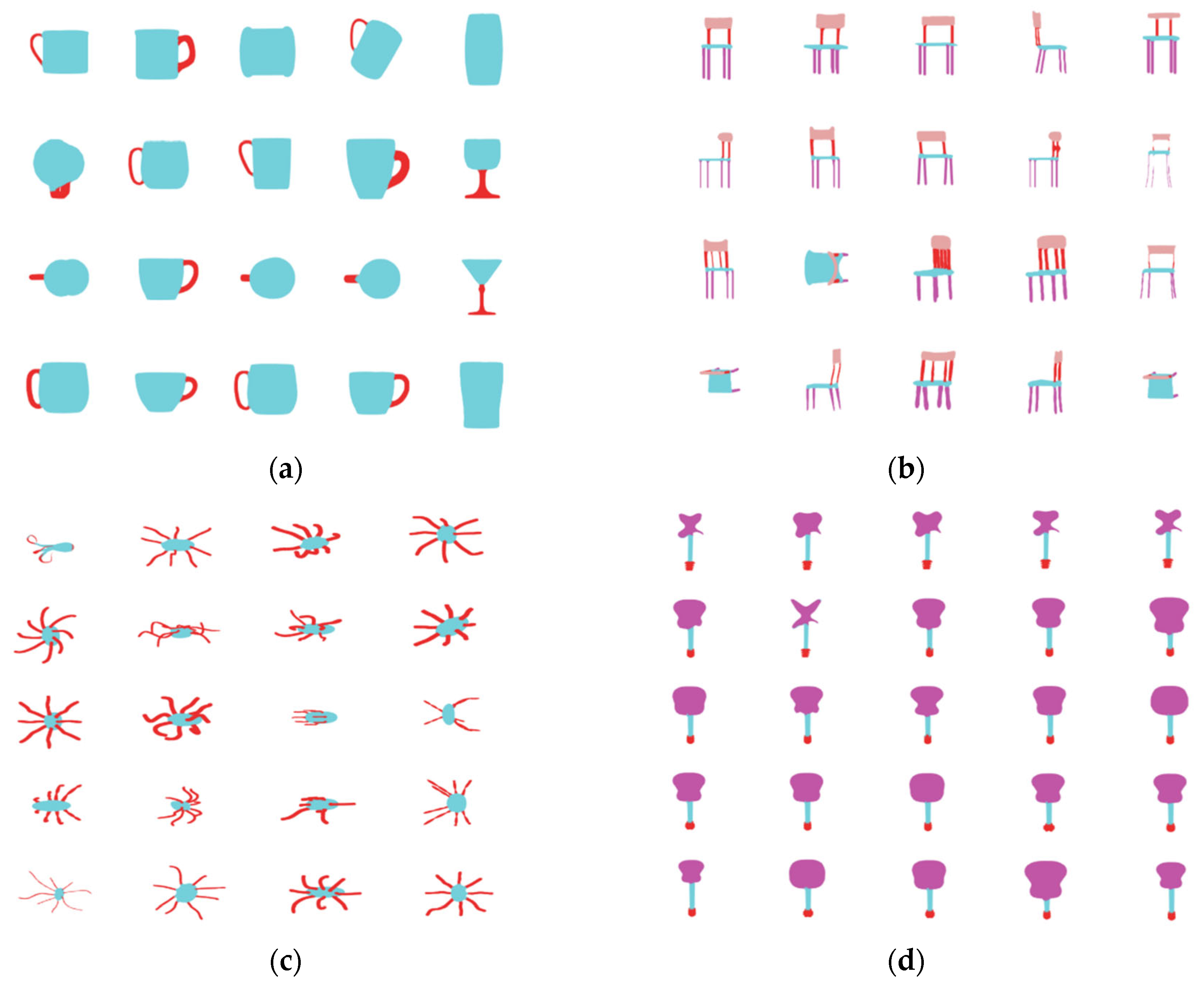
Table 2 and
Table 3 provide the segmentation accuracy for several categories within each PSB category and large datasets of COSEG. The bold numbers indicate the best results for each dataset, and ‘-’ indicates results that were not reported. On the PSB dataset, our proposed method achieves the best results in 8 out of 19 categories, and
Figure 8 shows some of the segmentation results of our algorithm on the PSB and COSEG datasets.
5.4. Ablation Study
The large COSEG dataset was used to evaluate the components in our network. The results of the evaluation are shown in
Table 3.
5.4.1. NGD-PE and Lap-PE
We compared the segmentation results of Lap-PE [
14] and NGD-PE.
Table 3 shows that our NGD-PE achieved better results than the Lap-PE. Furthermore, it is found that the performance improvement was limited when the N
u value of the NGD-PE was larger than the specified value. We also conducted experiments on the selection of α and achieved excellent results when the range was 0.5~2.
5.4.2. SAG Pooling vs. Top-K Pooling
We compared the two pooling algorithms, SAG pooling and Top-K pooling. SAG pooling has one more graph convolution operation than Top-K pooling.
Table 3 shows that SAG pooling performed better in these two pooling operations. At the same time, different K values were selected to observe their effects on performance. It is found that the performance improvement was relatively limited when the K value was greater than a specific value.
6. Conclusions and Discussion
This paper presented a novel transformer framework named NGD-Transformer for 3D triangle mesh. The framework bridges some critical gaps in the previous studies. First, the manifold preserved algorithm was used to split the shape into a sequence of uniform, non-overlapping patches. Second, the SAG pooling algorithm was used to generate tokens and raw feature embeddings. Third, to effectively capture the geodesic distance information, we designed NGD-PE to represent geodesic interactions between tokens. Finally, the subsequent neural networks were then constructed according to the classification and semantic segmentation tasks, respectively.
We also conducted complete experiments to test our proposed method. The experiments, which were conducted on multiple datasets, showed that our proposed network performs excellent classification and semantic segmentation. An ablation study on the NGD-PE module and the SAG pooling module was further conducted. It is found that NGD-PE can achieve better effects than Lap-PE and setting the appropriate number of sampling vertices and attenuation coefficient can further improve the segmentation effect. In addition, the input feature learning through GNN before Top-K pooling, that is, using SAG Pooling, can further improve the segmentation performance, and the improvement effect stabilizes when K is greater than a certain value. It is believed that this performance improvement mainly benefits from our learning of the manifold properties of shapes using the graph transformer network structure.
This improved segmentation performance allows our method to be further applied to shape deformation and shape animation, which often need to accurately identify the specific parts in the shape. The improvement of the classification performance enables our method to be applied to shape retrieval and to retrieve 3D shapes more accurately. Multiple extensions can be further explored. For example, our network can be used for shape completion. Our network divides shapes into multiple patches. If some patches are missing, our network can predict and complete the remaining patches combined with the mask mechanism. Our method can also be applied to shape correspondence, through which it can establish a patch-level correspondence through the analysis of the correlation between patches. Furthermore, since the transformer has been widely used in fields such as NLP and computer vision, our framework can be combined with NLP or computer vision to perform cross-modal learning.
Author Contributions
Conceptualization, J.Z. Funding acquisition, J.Z. and X.L. Methodology, J.Z. and X.L. Software, J.Z. Validation, W.Z. Writing—original draft, J.Z. and W.Z. Writing—review and editing, W.Z. All authors have read and agreed to the published version of the manuscript.
Funding
This work was supported by the Grants from the Education and Scientific Research Project for Middle-Aged and Young Teachers of Fujian Province (No. JAT210302); Innovation and Entrepreneurship Project for College Students (No. 202110399024); Fujian Province Science & Technology Program of China (2021H0053); and Quanzhou City Science & Technology Program of China (2020C019R, 2021C031R).
Conflicts of Interest
We declare that we have no financial and personal relationships with other people or organizations that can inappropriately influence our work; there is no professional or other personal interest of any nature or kind in any product, service and company that could be construed as influencing the position presented in, or the review of, the manuscript here entitled.
References
- Dai, Z.; Yang, Z.; Yang, Y.; Carbonell, J.; Salakhutdinov, R. Transformer-XL: Attentive Language Models beyond a Fixed-Length Context. arXiv 2019, arXiv:1901.02860. [Google Scholar]
- Devlin, J.; Chang, M.; Lee, K.; Toutanova, K. Bert: Pre-training of deep bidirectional transformers for language understanding. arXiv 2018, arXiv:1810.04805. [Google Scholar]
- Vaswani, A.; Shazeer, N.; Parmar, N.; Uszkoreit, J.; Jones, L.; Gomez, A.N.; Kaiser, Ł.; Polosukhin, I. Attention is all you need. Adv. Neural Inf. Process. Syst. 2017, 30, 1–15. [Google Scholar]
- Chen, H.; Wang, Y.; Guo, T.; Xu, C.; Deng, Y.; Liu, Z.; Ma, S.; Xu, C.; Xu, C.; Gao, W. Pre-trained image processing transformer. In Proceedings of the IEEE/CVF Conference on Computer Vision and Pattern Recognition, Nashville, TN, USA, 20–25 June 2021. [Google Scholar]
- Zheng, S.; Lu, J.; Zhao, H.; Zhu, X.; Luo, Z.; Wang, Y.; Fu, Y.; Feng, J.; Xiang, T.; Torr, P.H. Rethinking semantic segmentation from a sequence-to-sequence perspective with transformers. In Proceedings of the IEEE/CVF Conference on Computer Vision and Pattern Recognition, Nashville, TN, USA, 19–25 June 2021. [Google Scholar]
- Liu, Z.; Lin, Y.; Cao, Y.; Hu, H.; Wei, Y.; Zhang, Z.; Lin, S.; Guo, B. Swin transformer: Hierarchical vision transformer using shifted windows. In Proceedings of the IEEE/CVF International Conference on Computer Vision, Montreal, QC, Canada, 10–17 October 2021. [Google Scholar]
- Dosovitskiy, A.; Beyer, L.; Kolesnikov, A.; Weissenborn, D.; Zhai, X.; Unterthiner, T.; Dehghani, M.; Minderer, M.; Heigold, G.; Gelly, S. An image is worth 16 × 16 words: Transformers for image recognition at scale. arXiv 2020, arXiv:2010.11929. [Google Scholar]
- Carion, N.; Massa, F.; Synnaeve, G.; Usunier, N.; Kirillov, A.; Zagoruyko, S. End-to-end object detection with transformers. In Proceedings of the European Conference on Computer Vision, Glasgow, UK, 23–28 August 2020. [Google Scholar]
- Guo, M.; Cai, J.; Liu, Z.; Mu, T.; Martin, R.R.; Hu, S. PCT: Point cloud transformer. Comput. Vis. Media 2021, 7, 187–199. [Google Scholar] [CrossRef]
- Han, X.; Kuang, Y.; Xiao, G. Point cloud learning with transformer. arXiv 2021, arXiv:2104.13636. [Google Scholar]
- Han, X.; Jin, Y.; Cheng, H.; Xiao, G. Dual transformer for point cloud analysis. arXiv 2021, arXiv:2104.13044. [Google Scholar] [CrossRef]
- Zhao, H.; Jiang, L.; Jia, J.; Torr, P.H.; Koltun, V. Point transformer. In Proceedings of the IEEE/CVF International Conference on Computer Vision, Montreal, QC, Canada, 10–17 October 2021. [Google Scholar]
- Ying, C.; Cai, T.; Luo, S.; Zheng, S.; Ke, G.; He, D.; Shen, Y.; Liu, T. Do transformers really perform badly for graph representation? Adv. Neural Inf. Process. Syst. 2021, 34, 28877–28888. [Google Scholar]
- Kreuzer, D.; Beaini, D.; Hamilton, W.; Létourneau, V.; Tossou, P. Rethinking graph transformers with spectral attention. Adv. Neural Inf. Process. Syst. 2021, 34, 21618–21629. [Google Scholar]
- Dwivedi, V.P.; Bresson, X. A generalization of transformer networks to graphs. arXiv 2020, arXiv:2012.09699. [Google Scholar]
- Chen, D.; O’Bray, L.; Borgwardt, K. Structure-Aware Transformer for Graph Representation Learning. arXiv 2022, arXiv:2202.03036. [Google Scholar]
- Zhang, J.; Zhang, H.; Xia, C.; Sun, L. Graph-bert: Only attention is needed for learning graph representations. arXiv 2020, arXiv:2001.05140. [Google Scholar]
- Knyazev, B.; Taylor, G.W.; Amer, M. Understanding attention and generalization in graph neural networks. Adv. Neural Inf. Process. Syst. 2019, 32, 1–11. [Google Scholar]
- Gou, B.; Cheng, Y.; de Ruiter, A.H.J. INS/CNS navigation system based on multi-star pseudo measurements. Aerosp. Sci. Technol. 2019, 95, 105506. [Google Scholar] [CrossRef]
- Huang, H.; Fang, Y. Adaptive Wavelet Transformer Network for 3D Shape Representation Learning. In Proceedings of the International Conference on Learning Representations, Vienna, Austria, 3–7 May 2021. [Google Scholar]
- Shajahan, D.A.; Varma, M.; Muthuganapathy, R. Point transformer for shape classification and retrieval of urban roof point clouds. IEEE Geosci. Remote Sens. Lett. 2021, 19, 1–5. [Google Scholar] [CrossRef]
- Yan, X.; Lin, L.; Mitra, N.J.; Lischinski, D.; Cohen-Or, D.; Huang, H. Shapeformer: Transformer-based shape completion via sparse representation. In Proceedings of the IEEE/CVF Conference on Computer Vision and Pattern Recognition, New Orleans, LA, USA, 19–24 June 2022. [Google Scholar]
- Sarasua, I.; Pölsterl, S.; Wachinger, C.; Alzheimer, S.D.N. Transformesh: A transformer network for longitudinal modeling of anatomical meshes. In Proceedings of the International Workshop on Machine Learning in Medical Imaging, Strasbourg, France, 27 September 2021; pp. 209–218. [Google Scholar]
- Lin, K.; Wang, L.; Liu, Z. Mesh graphormer. In Proceedings of the IEEE/CVF International Conference on Computer Vision, Montreal, QC, Canada, 10–17 October 2021. [Google Scholar]
- He, L.; Dong, Y.; Wang, Y.; Tao, D.; Lin, Z. Gauge equivariant transformer. Adv. Neural Inf. Process. Syst. 2021, 34, 27331–27343. [Google Scholar]
- Liang, Y.; Zhao, S.; Yu, B.; Zhang, J.; He, F. MeshMAE: Masked Autoencoders for 3D Mesh Data Analysis. arXiv 2022, arXiv:2207.10228. [Google Scholar]
- Qiao, Y.L.; Gao, L.; Yang, J.; Rosin, P.L.; Lai, Y.K.; Chen, X. Learning on 3D Meshes With Laplacian Encoding and Pooling. IEEE Trans. Vis. Comput. Graph. 2022, 28, 1317–1327. [Google Scholar] [CrossRef]
- Dhillon, I.S.; Guan, Y.; Kulis, B. Weighted graph cuts without eigenvectors a multilevel approach. IEEE Trans. Pattern Anal. Mach. Intell. 2007, 29, 1944–1957. [Google Scholar] [CrossRef]
- Ranjan, A.; Bolkart, T.; Sanyal, S.; Black, M.J. Generating 3D faces using convolutional mesh autoencoders. In Proceedings of the European Conference on Computer Vision (ECCV), Munich, Germany, 8–14 September 2018. [Google Scholar]
- Hanocka, R.; Hertz, A.; Fish, N.; Giryes, R.; Fleishman, S.; Cohen-Or, D. MeshCNN: A network with an edge. ACM Trans. Graph. 2019, 38, 1–12. [Google Scholar] [CrossRef] [Green Version]
- Poulenard, A.; Ovsjanikov, M. Multi-directional geodesic neural networks via equivariant convolution. ACM Trans. Graph. 2018, 37, 1–14. [Google Scholar] [CrossRef] [Green Version]
- Schult, J.; Engelmann, F.; Kontogianni, T.; Leibe, B. DualConvMesh-Net: Joint Geodesic and Euclidean Convolutions on 3D Meshes. In Proceedings of the IEEE/CVF Conference on Computer Vision and Pattern Recognition, Seattle, WA, USA, 13–19 June 2020. [Google Scholar]
- Mialon, G.; Chen, D.; Selosse, M.; Mairal, J. Graphit: Encoding graph structure in transformers. arXiv 2021, arXiv:2106.05667. [Google Scholar]
- Wu, Z.; Jain, P.; Wright, M.; Mirhoseini, A.; Gonzalez, J.E.; Stoica, I. Representing long-range context for graph neural networks with global attention. Adv. Neural Inf. Process. Syst. 2021, 34, 13266–13279. [Google Scholar]
- Min, E.; Chen, R.; Bian, Y.; Xu, T.; Zhao, K.; Huang, W.; Zhao, P.; Huang, J.; Ananiadou, S.; Rong, Y. Transformer for Graphs: An Overview from Architecture Perspective. arXiv 2022, arXiv:2202.08455. [Google Scholar]
- Kalogerakis, E.; Hertzmann, A.; Singh, K. Learning 3D Mesh Segmentation and Labeling. ACM Trans. Graph. 2010, 29, 1–12. [Google Scholar] [CrossRef]
- Huang, J.; Su, H.; Guibas, L. Robust watertight manifold surface generation method for shapenet models. arXiv 2018, arXiv:1802.01698. [Google Scholar]
- Aubry, M.; Schlickewei, U.; Cremers, D. The wave kernel signature: A quantum mechanical approach to shape analysis. In Proceedings of the 2011 IEEE International Conference on Computer Vision Workshops (ICCV Workshops), Barcelona, Spain, 6–13 November 2011. [Google Scholar]
- Johnson, A.E. Spin-Images: A Representation for 3-D Surface Matching. Ph.D. Thesis, Robotics Institute Carnegie Mellon University, Pittsburgh, PA, USA, 1997. [Google Scholar]
- Defferrard, M.; Bresson, X.; Vandergheynst, P. Convolutional neural networks on graphs with fast localized spectral filtering. Adv. Neural Inf. Process. Syst. 2016, 29, 1–9. [Google Scholar]
- Wu, Z.; Song, S.; Khosla, A.; Yu, F.; Zhang, L.; Tang, X.; Xiao, J. 3D ShapeNets: A Deep Representation for Volumetric Shapes. In Proceedings of the IEEE Conference on Computer Vision and Pattern Recognition, Boston, MA, USA, 7–12 June 2015. [Google Scholar]
- Qi, C.R.; Li, Y.; Hao, S.; Guibas, L.J. PointNet++: Deep Hierarchical Feature Learning on Point Sets in a Metric Space. Adv. Neural Inf. Process. Syst. 2017, 30, 1–10. [Google Scholar]
- Maturana, D.; Scherer, S. VoxNet: A 3D Convolutional Neural Network for real-time object recognition. In Proceedings of the 2015 IEEE/RSJ International Conference on Intelligent Robots and Systems (IROS), Hamburg, Germany, 28 September–2 October 2015. [Google Scholar]
- Hu, S.; Liu, Z.; Guo, M.; Cai, J.; Huang, J.; Mu, T.; Martin, R.R. Subdivision-Based Mesh Convolution Networks. ACM Trans. Graph. 2021, 1, 1–16. [Google Scholar] [CrossRef]
- Chen, X.; Golovinskiy, A.; Funkhouser, T.A. A benchmark for 3D mesh segmentation. ACM Trans. Graph. 2009, 28, 1–12. [Google Scholar]
- Wang, Y.; Asafi, S.; van Kaick, O.; Zhang, H.; Cohen-Or, D.; Chen, B. Active co-analysis of a set of shapes. ACM Trans. Graph. 2012, 31, 1–10. [Google Scholar] [CrossRef] [Green Version]
- Guo, K.; Zou, D.; Chen, X. 3D Mesh Labeling via Deep Convolutional Neural Networks. ACM Trans. Graph. 2015, 35, 1–12. [Google Scholar] [CrossRef]
- Kalogerakis, E.; Averkiou, M.; Maji, S.; Chaudhuri, S. 3D Shape Segmentation with Projective Convolutional Networks. In Proceedings of the IEEE Conference on Computer Vision and Pattern Recognition, Honolulu, HI, USA, 21–26 July 2017. [Google Scholar]
- Milano, F.; Loquercio, A.; Vidal, A.R.; Scaramuzza, D.; Carlone, L. Primal-Dual Mesh Convolutional Neural Networks. Adv. Neural Inf. Process. Syst. 2020, 33, 952–963. [Google Scholar]
| Publisher’s Note: MDPI stays neutral with regard to jurisdictional claims in published maps and institutional affiliations. |
© 2022 by the authors. Licensee MDPI, Basel, Switzerland. This article is an open access article distributed under the terms and conditions of the Creative Commons Attribution (CC BY) license (https://creativecommons.org/licenses/by/4.0/).


