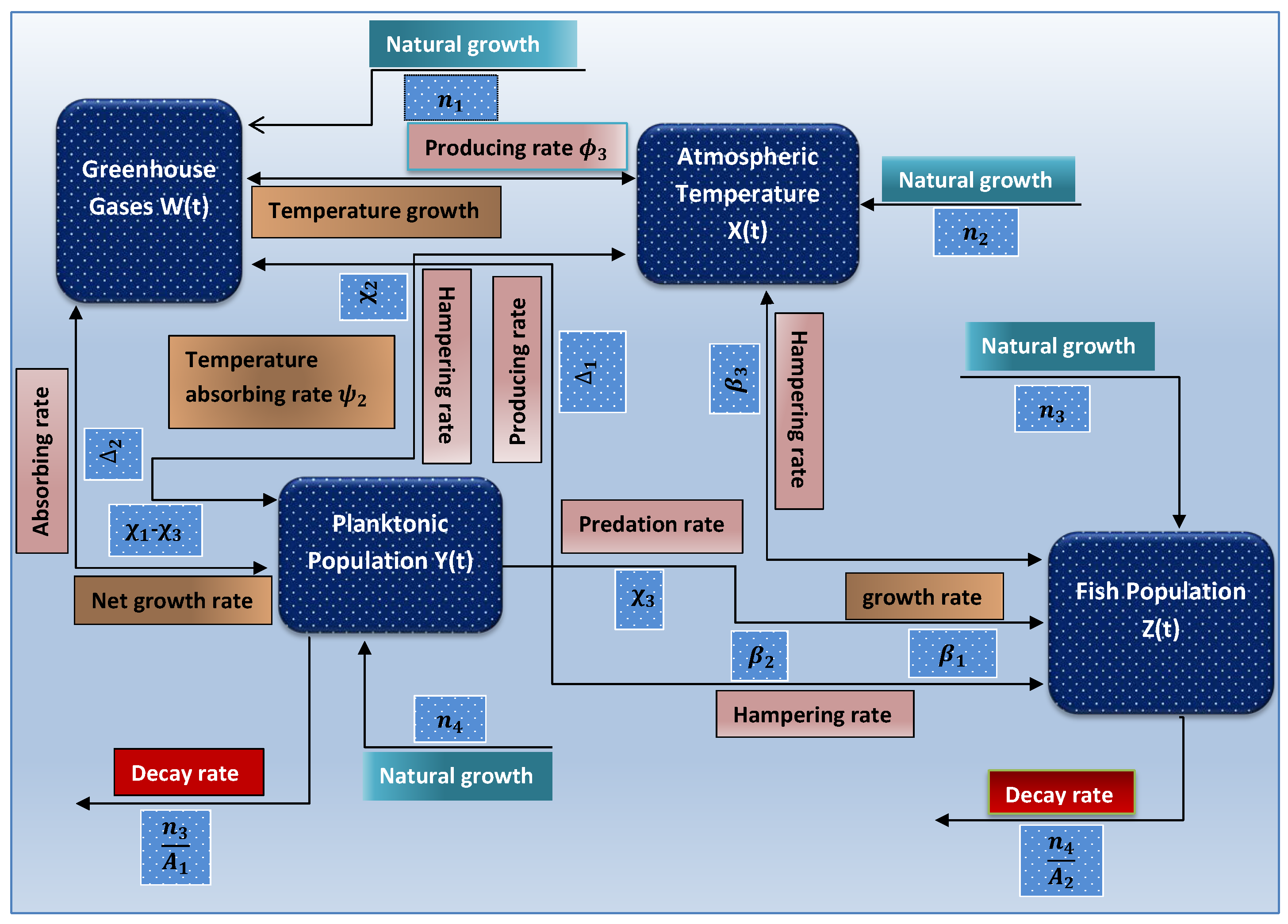
Figure 1.
Schematic diagram of Model (
1) showing the effect of greenhouse gas on temperature rise and the effect on marine environment and fishing community [
16].
Figure 1.
Schematic diagram of Model (
1) showing the effect of greenhouse gas on temperature rise and the effect on marine environment and fishing community [
16].
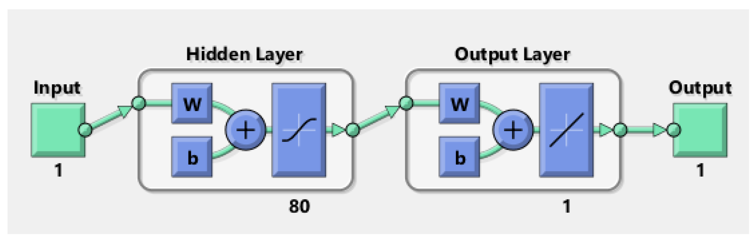
Figure 2.
Architecture of artificial neural networks with single neuron.
Figure 2.
Architecture of artificial neural networks with single neuron.
Figure 3.
Neural networks architecture.
Figure 3.
Neural networks architecture.
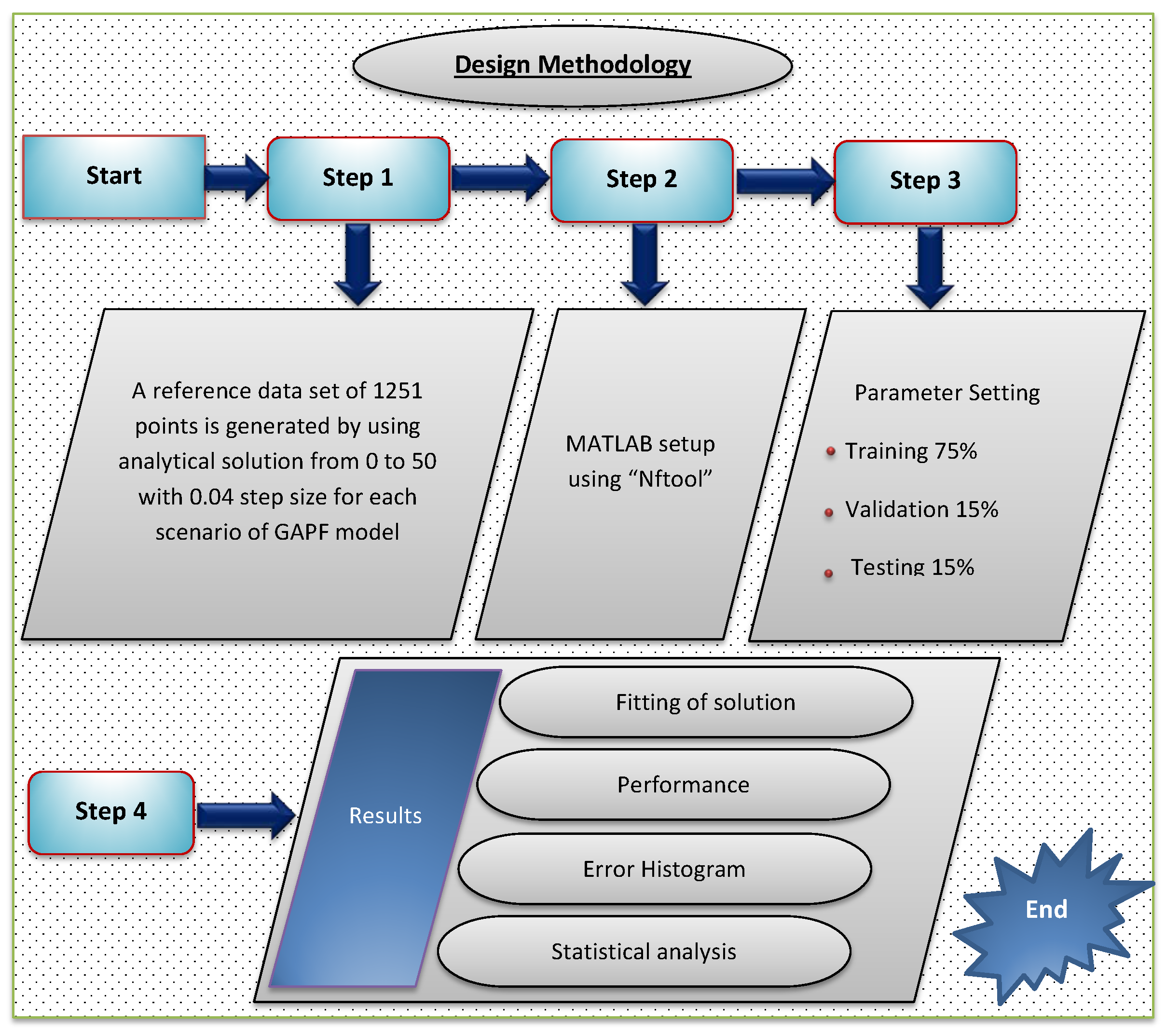
Figure 4.
Flow chart for the design methodology.
Figure 4.
Flow chart for the design methodology.
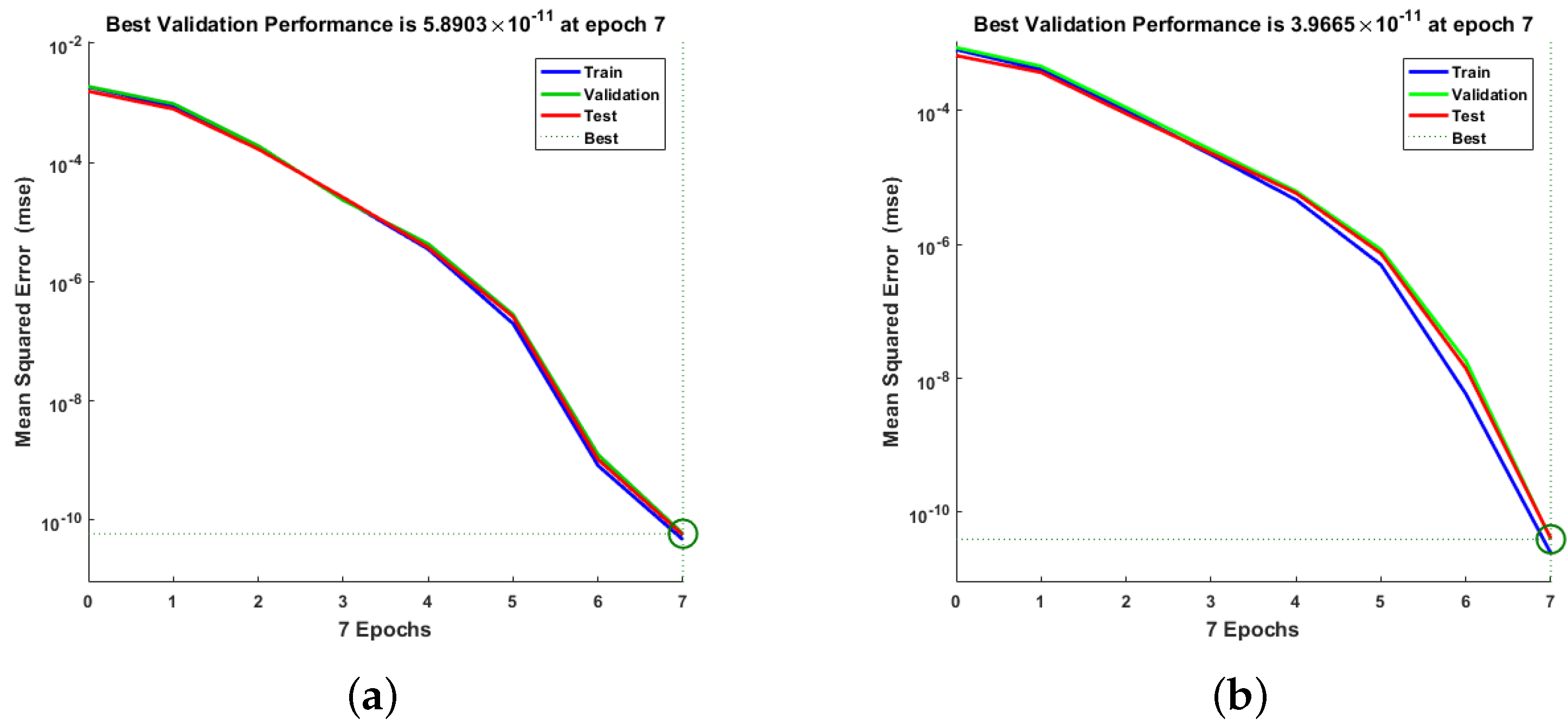
Figure 5.
Mean square error of RP-LMS through NNs for greenhouse gases and ambient temperature for Scenario 1. (a) W(t); (b) X(t).
Figure 5.
Mean square error of RP-LMS through NNs for greenhouse gases and ambient temperature for Scenario 1. (a) W(t); (b) X(t).
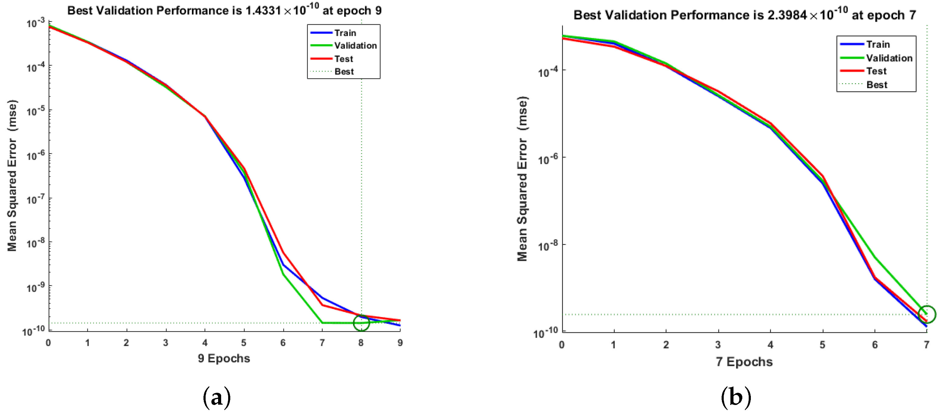
Figure 6.
Mean square error of RP-LMS through NNs for aquatic population and fish population for Scenario 1. (a) Y(t), (b) Z(t).
Figure 6.
Mean square error of RP-LMS through NNs for aquatic population and fish population for Scenario 1. (a) Y(t), (b) Z(t).
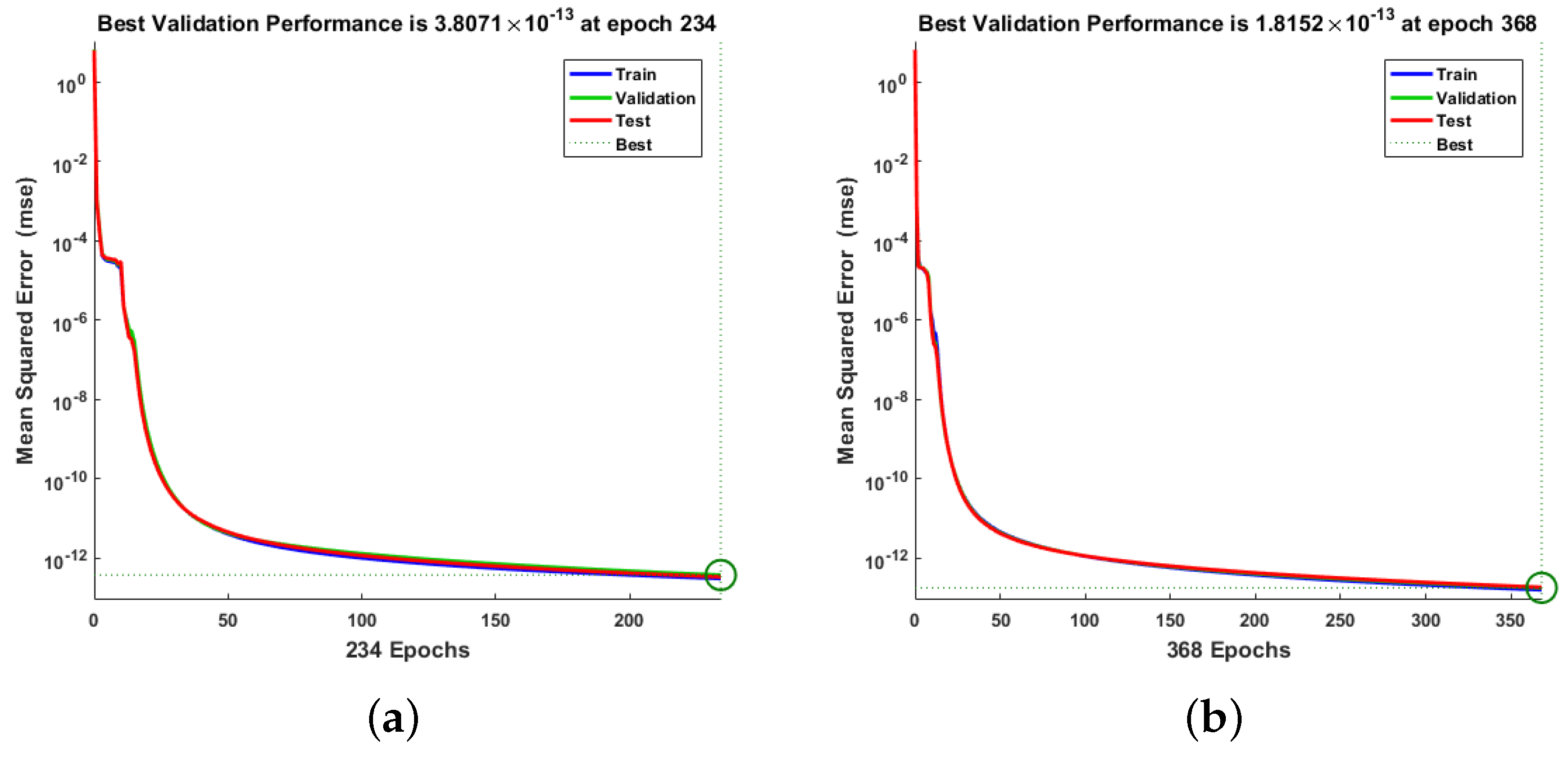
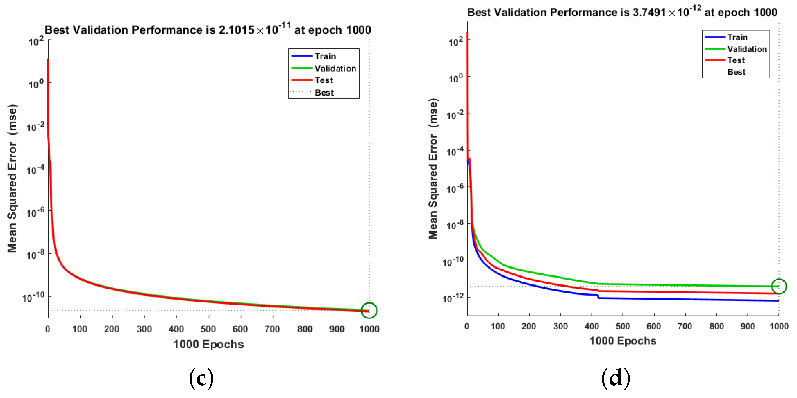
Figure 7.
Mean square error of RP-LMS through NNs for greenhouse gases, ambient temperature, aquatic population, and fish population for Scenario 2. (a) W(t), (b) X(t), (c) Y(t), (d) Z(t).
Figure 7.
Mean square error of RP-LMS through NNs for greenhouse gases, ambient temperature, aquatic population, and fish population for Scenario 2. (a) W(t), (b) X(t), (c) Y(t), (d) Z(t).
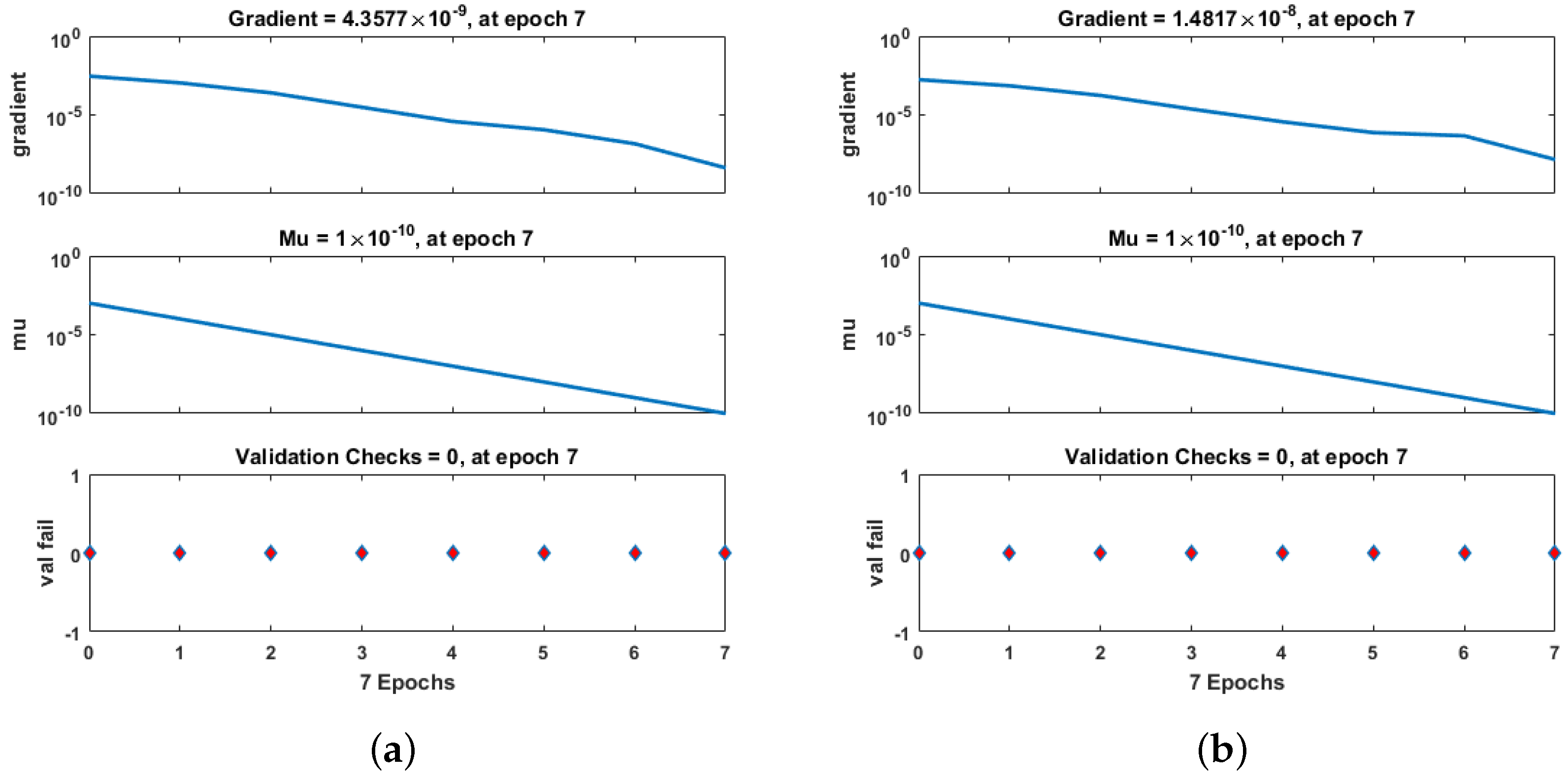
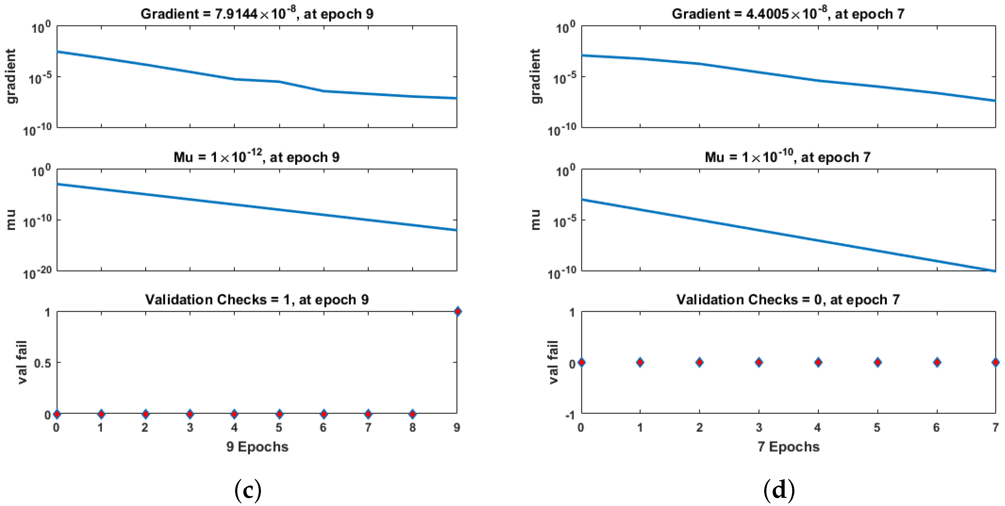
Figure 8.
Performance of RP-LMS through SNN in terms of mu, gradient, and validation checks for greenhouse gases, ambient temperature, aquatic population, and fish population for Case 1. (a) W(t), (b) X(t), (c) Y(t), (d) Z(t).
Figure 8.
Performance of RP-LMS through SNN in terms of mu, gradient, and validation checks for greenhouse gases, ambient temperature, aquatic population, and fish population for Case 1. (a) W(t), (b) X(t), (c) Y(t), (d) Z(t).
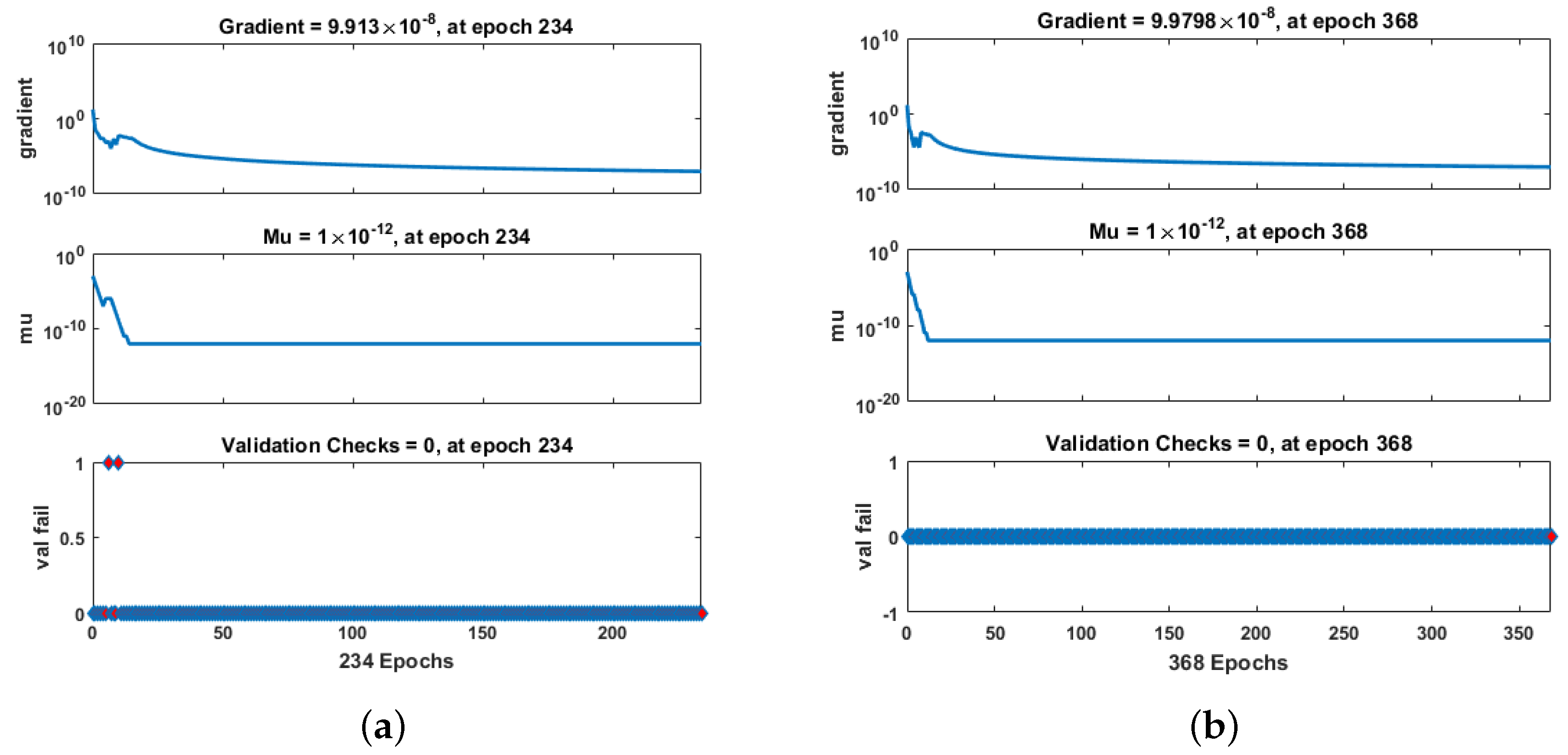
Figure 9.
Performance of RP-LMS through SNN in terms of mu, gradient, and validation checks for greenhouse gases and ambient temperature for Case 2. (a) W(t), (b) X(t).
Figure 9.
Performance of RP-LMS through SNN in terms of mu, gradient, and validation checks for greenhouse gases and ambient temperature for Case 2. (a) W(t), (b) X(t).
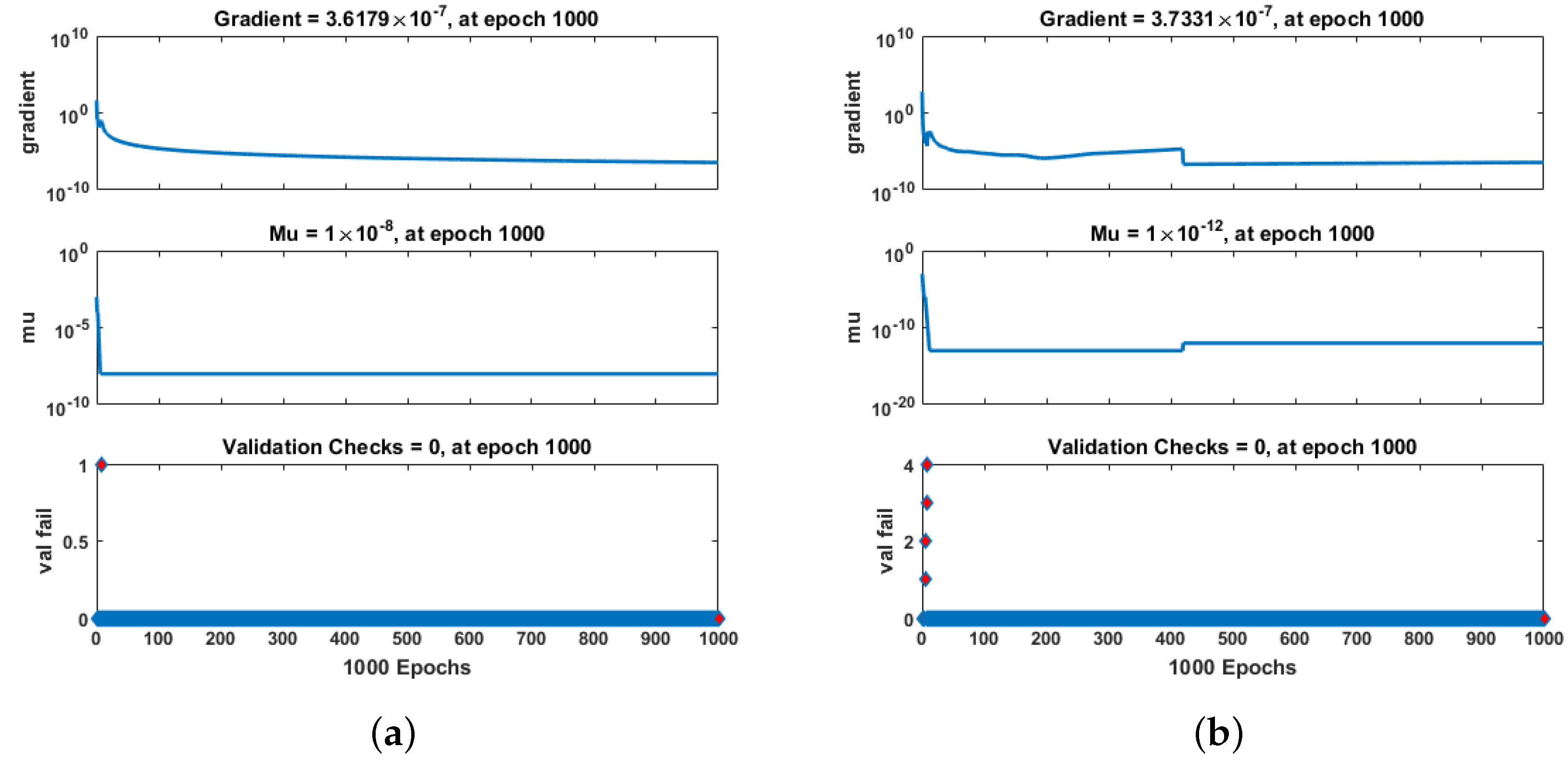
Figure 10.
Performance of RP-LMA through SNN in terms of mu, gradient, and validation checks for aquatic population, and fish population for Case 2. (a) Y(t), (b) Z(t).
Figure 10.
Performance of RP-LMA through SNN in terms of mu, gradient, and validation checks for aquatic population, and fish population for Case 2. (a) Y(t), (b) Z(t).
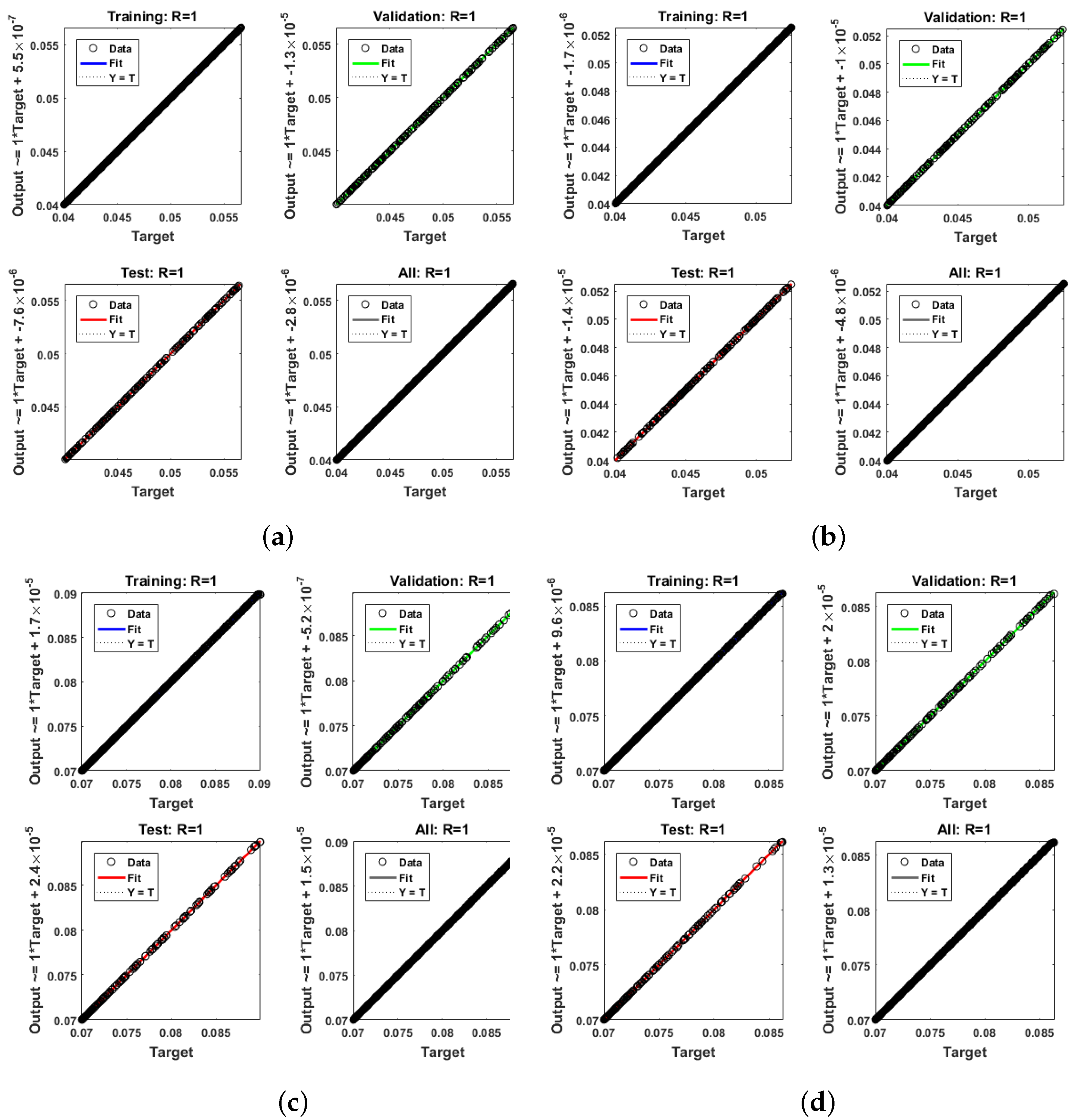
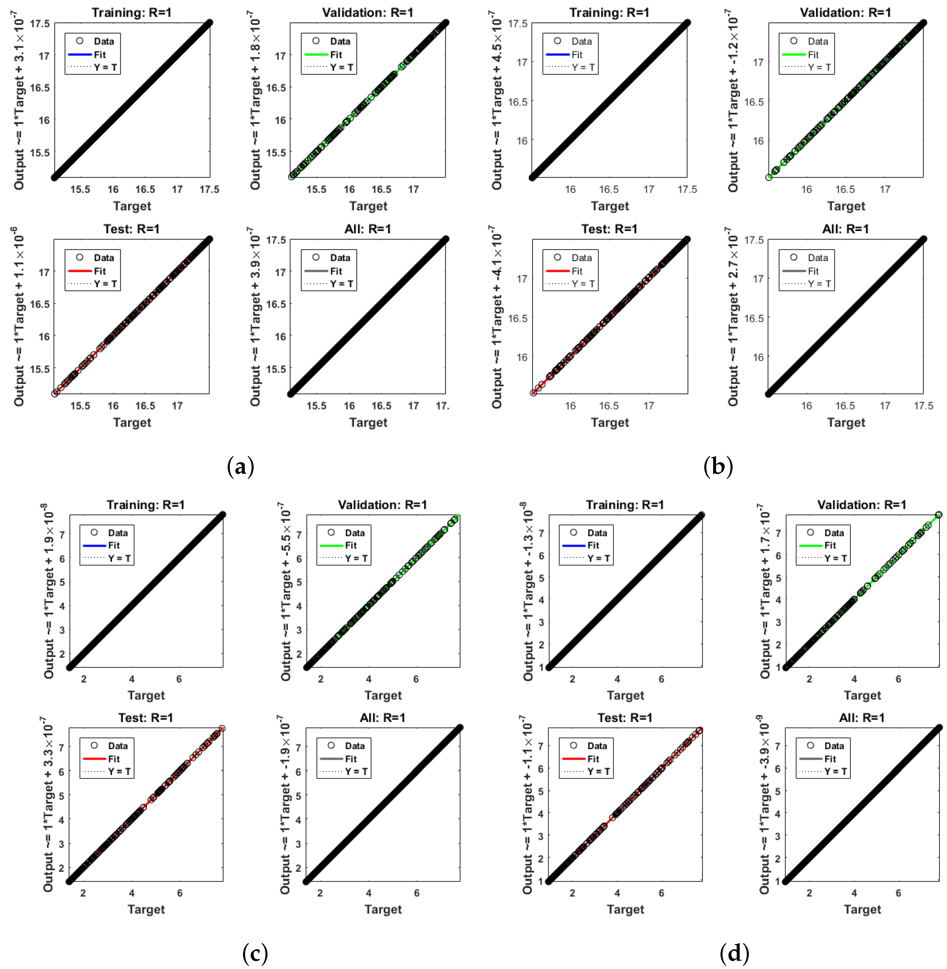
Figure 11.
Regression analysis of RP-LMS through SNN for training, validation, testing, and all samples, respectively, for the GAPF model in Case 1. (a) W(t), (b) X(t), (c) Y(t), (d) Z(t).
Figure 11.
Regression analysis of RP-LMS through SNN for training, validation, testing, and all samples, respectively, for the GAPF model in Case 1. (a) W(t), (b) X(t), (c) Y(t), (d) Z(t).
Figure 12.
Regression analysis of RP-LMS through SNN for training, validation, testing, and all samples, respectively, for the GAPF model in Case 2. (a) W(t), (b) X(t), (c) Y(t), (d) Z(t).
Figure 12.
Regression analysis of RP-LMS through SNN for training, validation, testing, and all samples, respectively, for the GAPF model in Case 2. (a) W(t), (b) X(t), (c) Y(t), (d) Z(t).
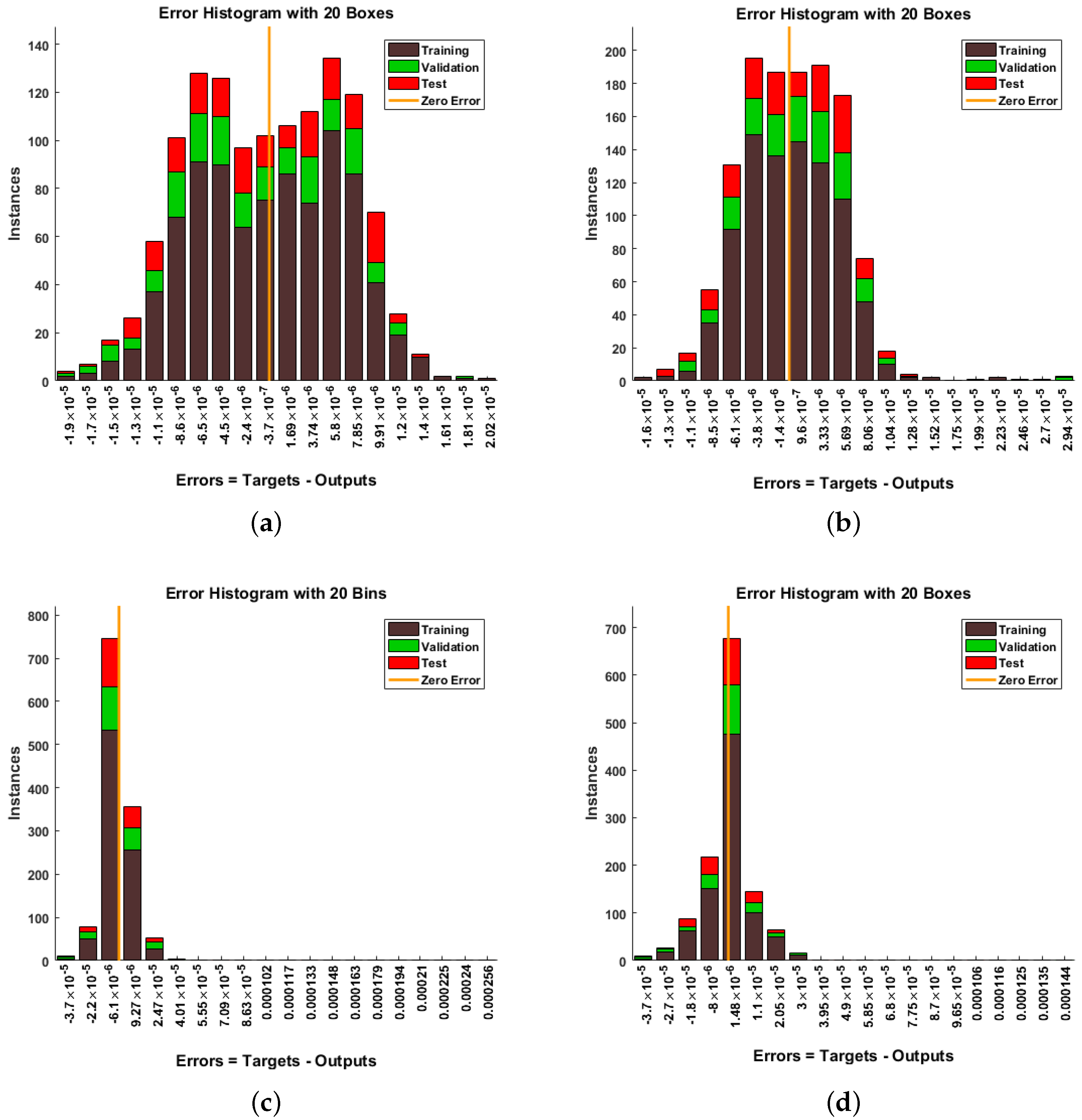
Figure 13.
Error histogram for the proposed methodology in terms of greenhouse gases, ambient temperature, aquatic population, and fish population for Case Study 1. (a) W(t), (b) X(t), (c) Y(t), (d) Z(t).
Figure 13.
Error histogram for the proposed methodology in terms of greenhouse gases, ambient temperature, aquatic population, and fish population for Case Study 1. (a) W(t), (b) X(t), (c) Y(t), (d) Z(t).
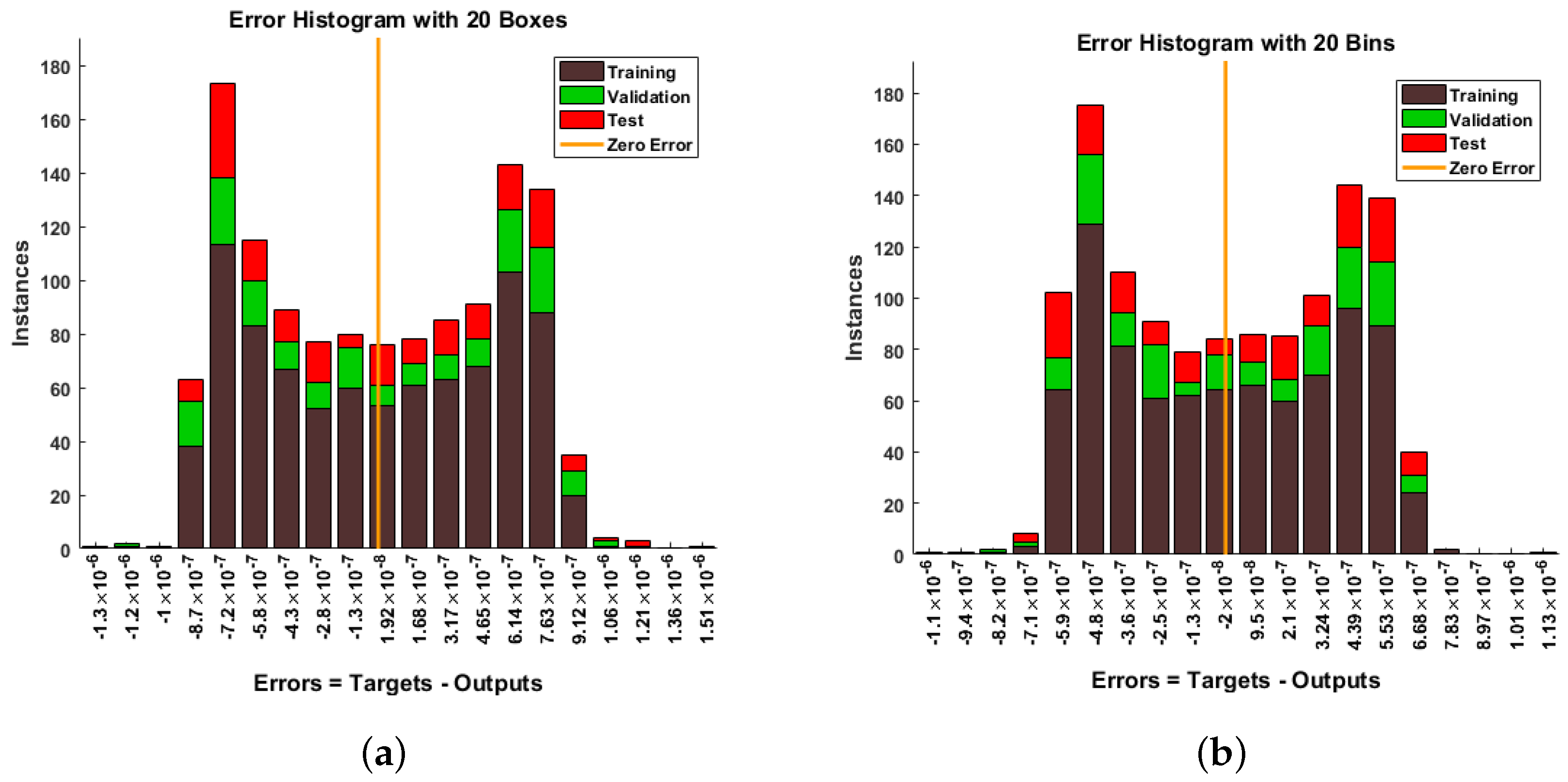
Figure 14.
Error histogram for the proposed methodology in terms of greenhouse gases and ambient temperature for Case Study 2. (a) W(t), (b) X(t).
Figure 14.
Error histogram for the proposed methodology in terms of greenhouse gases and ambient temperature for Case Study 2. (a) W(t), (b) X(t).
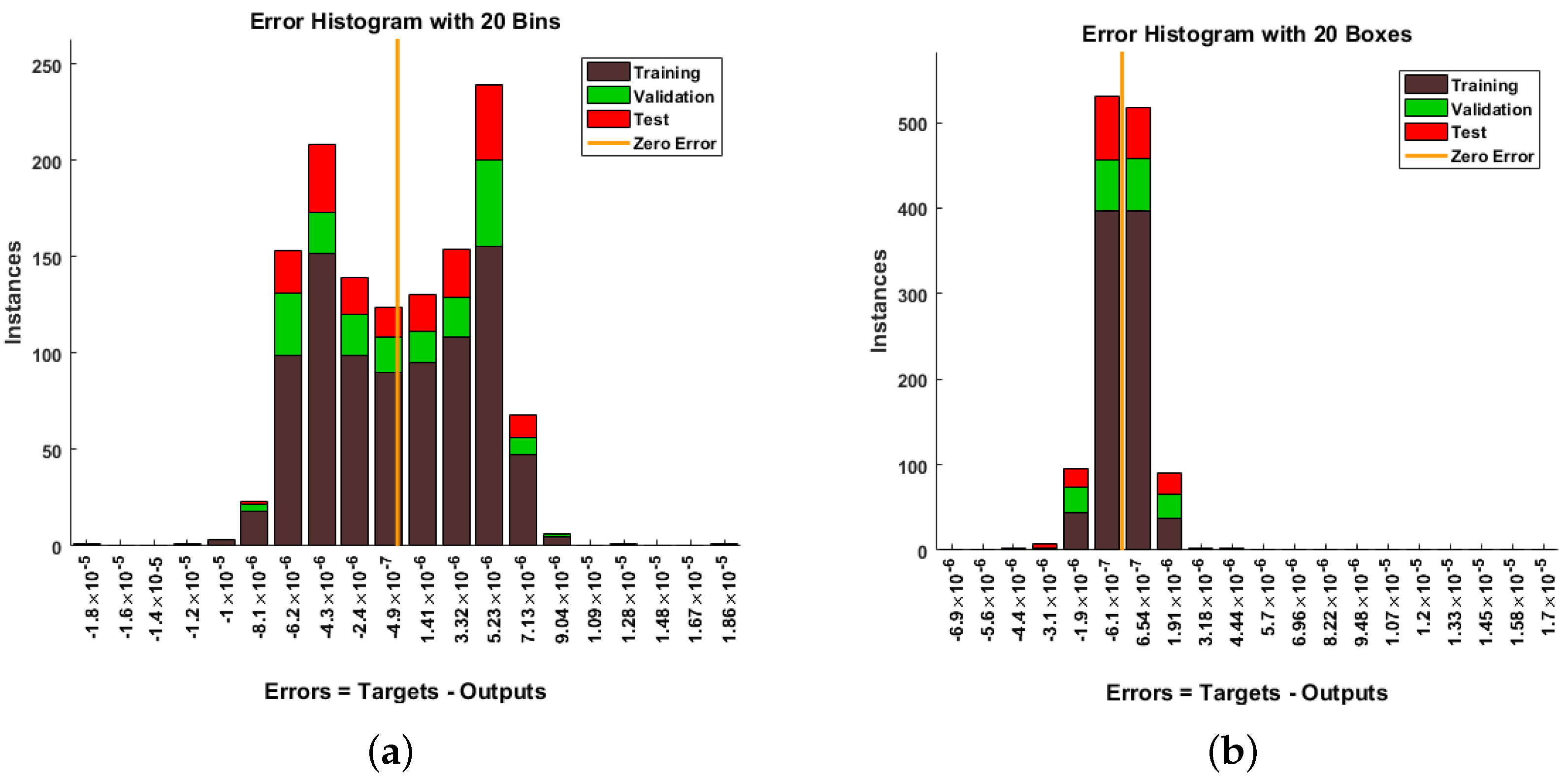
Figure 15.
Error histogram for the proposed methodology in terms of aquatic population and fish population for Case Study 2. (a) Y(t), (b) Z(t).
Figure 15.
Error histogram for the proposed methodology in terms of aquatic population and fish population for Case Study 2. (a) Y(t), (b) Z(t).
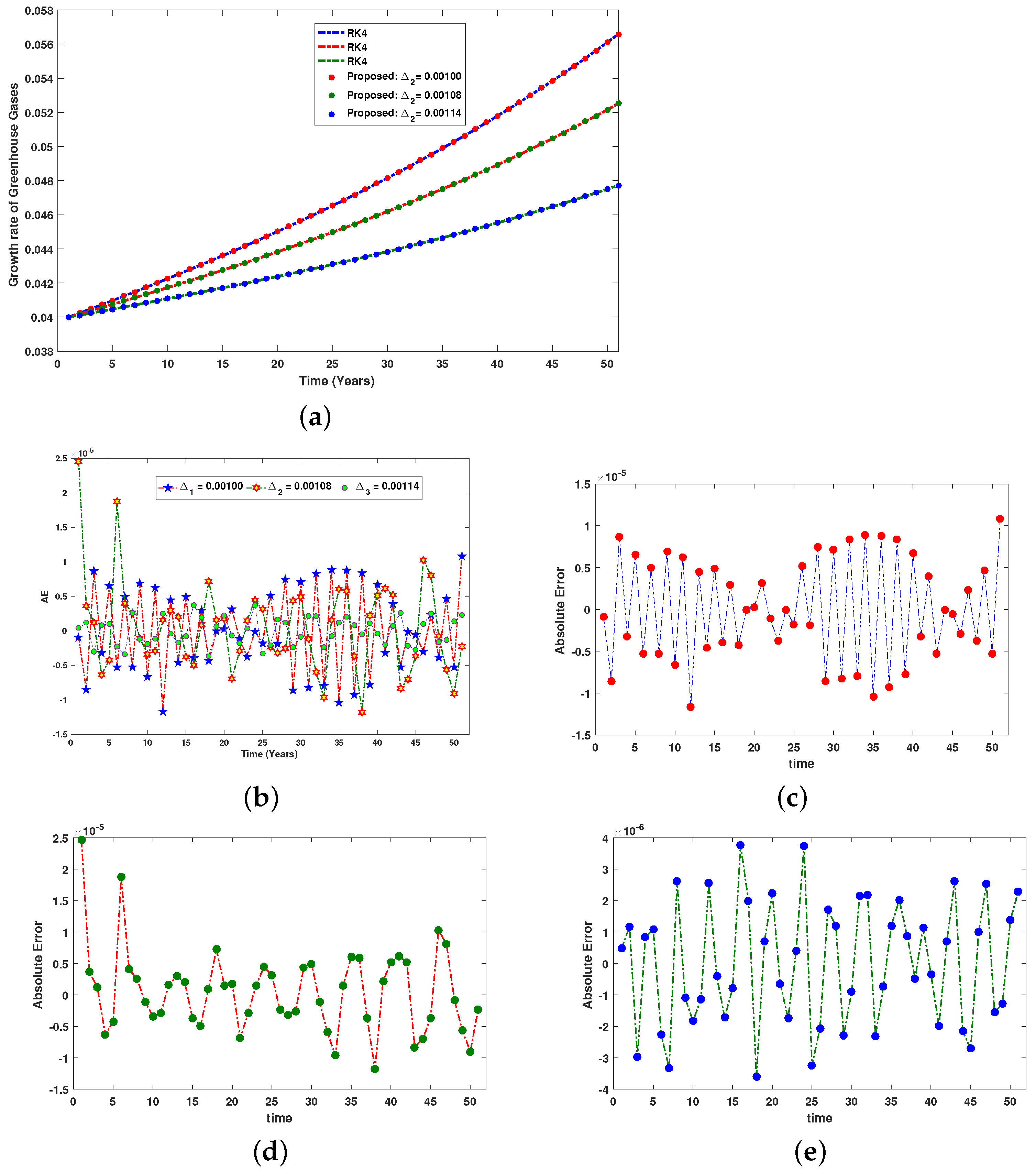
Figure 16.
Comparison between the numerical reference solution and the proposed RP-LMS through SNN for greenhouse gases. (a) Impact of on greenhouse gases, (b) collective analysis of Absolute Error, (c) analysis of case 1’s errors, (d) analysis of case 2’s errors, (e) analysis of case 3’s errors.
Figure 16.
Comparison between the numerical reference solution and the proposed RP-LMS through SNN for greenhouse gases. (a) Impact of on greenhouse gases, (b) collective analysis of Absolute Error, (c) analysis of case 1’s errors, (d) analysis of case 2’s errors, (e) analysis of case 3’s errors.
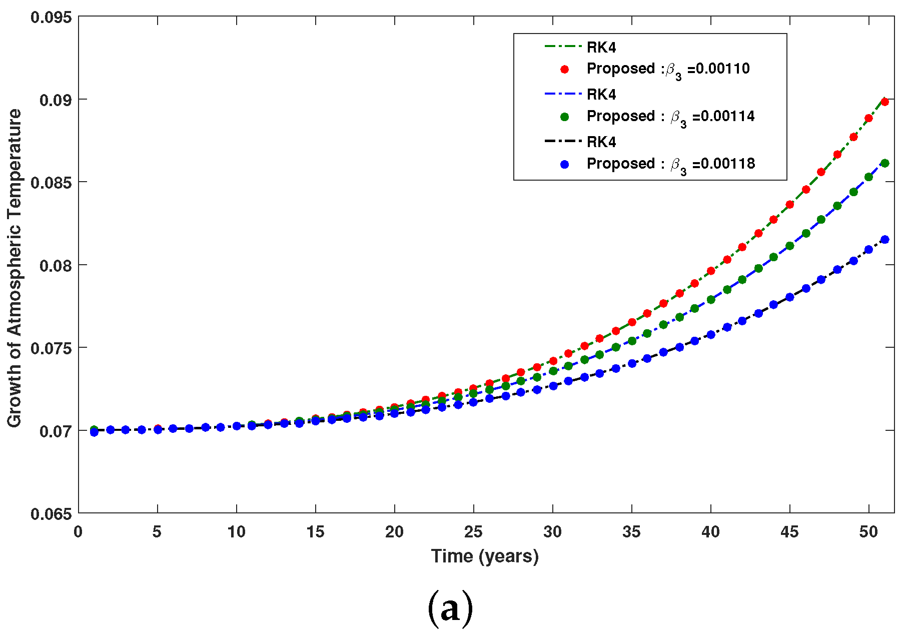
Figure 17.
Comparison between the numerical reference solution and the proposed RP-LMS through SNN for ambient temperature. (a) Impact of on atmospheric temperature, (b) collective analysis of Absolute Error, (c) analysis of case 1’s errors, (d) analysis of case 2’s errors, (e) analysis of case 3’s errors.
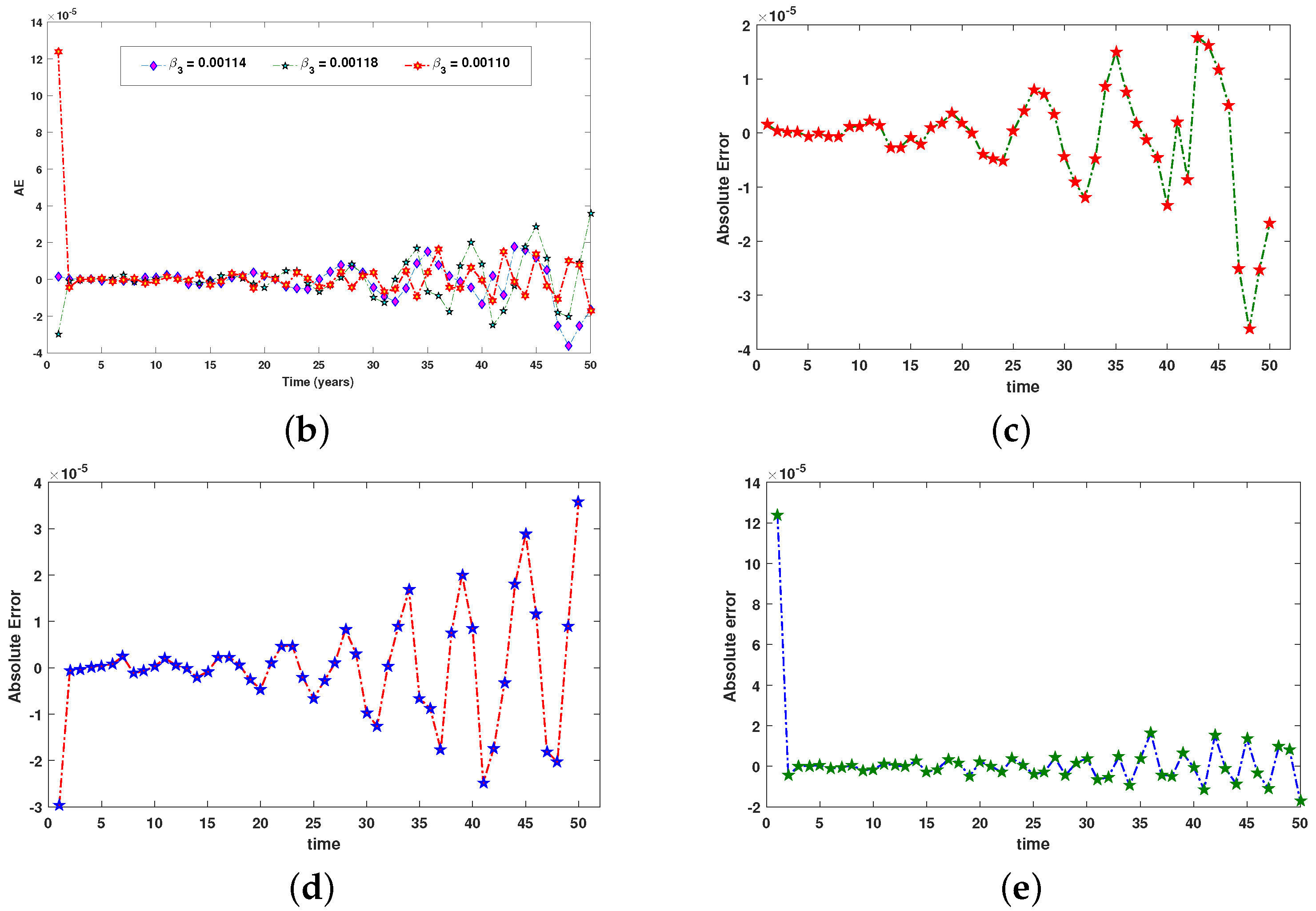
Figure 18.
Comparison between the numerical reference solution and the proposed RP-LMS through SNN for aquatic population. (a) Impact of on planktonic population, (b) collective analysis of Absolute Error, (c) analysis of case 1’s errors, (d) analysis of case 2’s errors, (e) analysis of case 3’s errors.
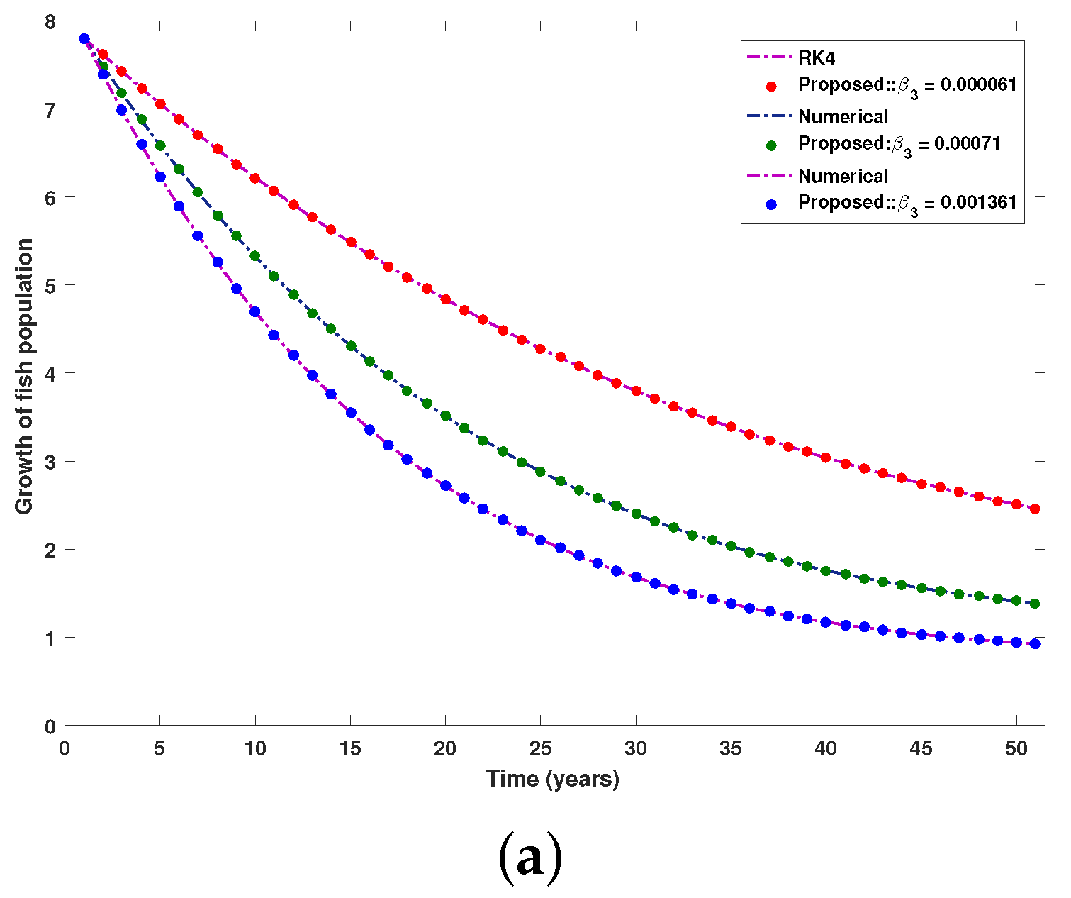
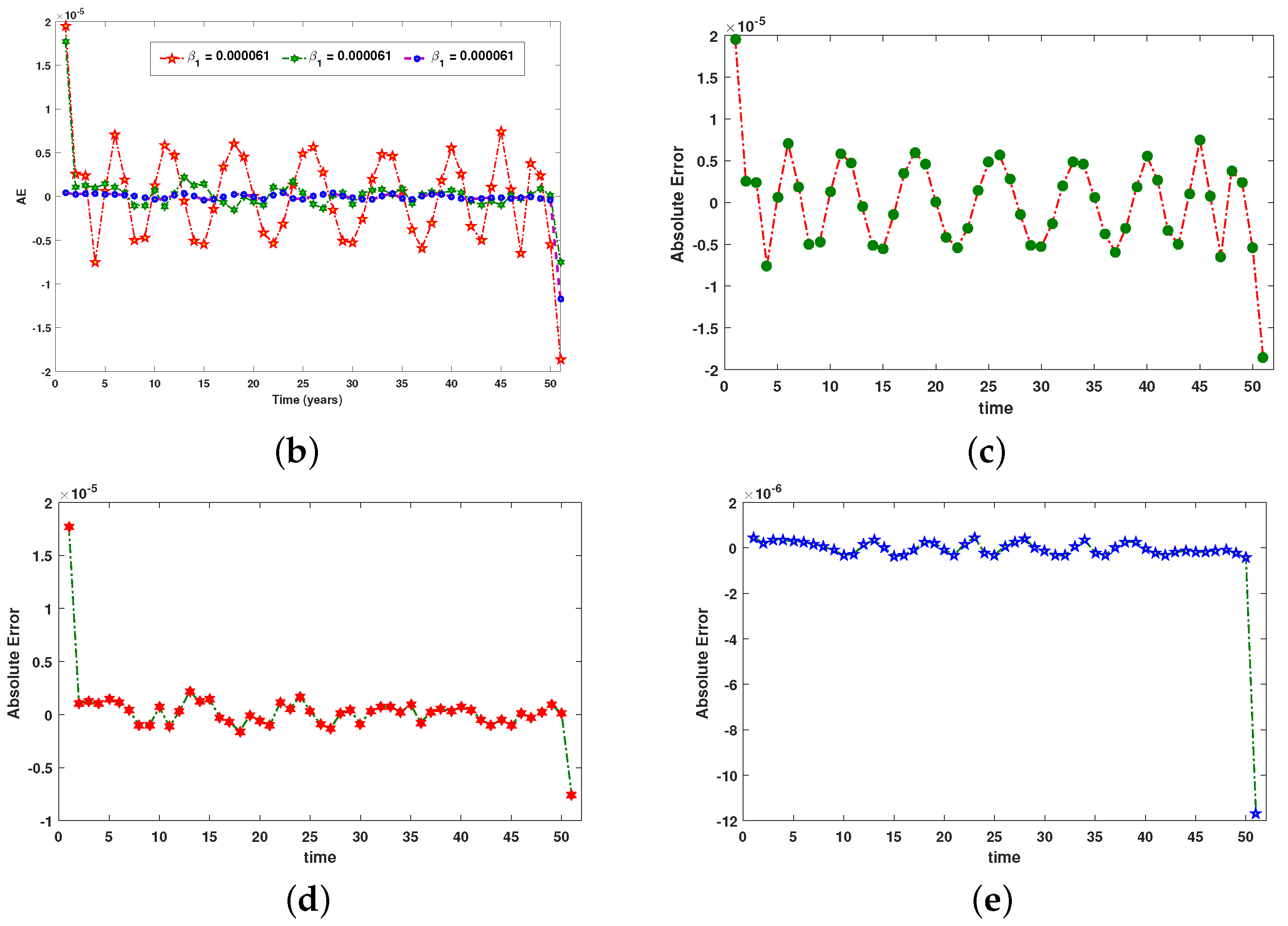
Figure 19.
Comparison between the numerical reference solution and the proposed RP-LMS through SNN for fish population. (a) Impact of on fish population, (b) collective analysis of Absolute Error, (c) analyze of error for case 1, (d) analyze of error for case 2, (e) analyze of error for case 3.
Figure 19.
Comparison between the numerical reference solution and the proposed RP-LMS through SNN for fish population. (a) Impact of on fish population, (b) collective analysis of Absolute Error, (c) analyze of error for case 1, (d) analyze of error for case 2, (e) analyze of error for case 3.
Table 1.
Previous studies compared to this study.
Table 1.
Previous studies compared to this study.
| Literature | Parameter Growth Rate of | Effect of Climate Change | Solution | Case |
|---|
| Review | Growth and Rate of Decline | on Marine Ecosystem | Type | Study |
|---|
| | Secondary | Measured | Global Warming | Marine Plankton | Fish Community | Exact | Heuristic | |
| Hinners et al. [25] | Yes | No | Yes | Yes | No | Yes | No | No |
| Asch et al. [10] | Yes | No | Yes | Yes | Yes | No | No | No |
| Mandal et al. [16] | No | Yes | Yes | Yes | No | Yes | No | No |
| Speers et al. [8] | Yes | No | Yes | Yes | Yes | Yes | No | No |
| Sekerci and | No | Yes | Yes | Yes | No | Yes | No | No |
| Petrovskii [13] | | | | | | | | |
| This study | No | Yes | Yes | Yes | Yes | Yes | Yes | Yes |
Table 2.
Describe the relevant values of the parameters used in this study.
Table 2.
Describe the relevant values of the parameters used in this study.
| Symbols | Descriptions | Values |
|---|
| GHG levels in the oceans are naturally growing. | 0.00095 kg/km |
| Plankton-feeding fish growth during the period | 0.099 C |
| The normal rate of expansion of the aquatic species | 0.00225 km |
| The perfectly natural increase in the population of fish | 0.0002/1000 |
| The oceanic aquatic demographic’s rate of GHG production | 0.0029 kg/km |
| GHG absorption rate by planktonic populations in the oceans | 0.00099 kg/km |
| Due to rising temperatures, the rate at which GHGs are emitted | 1.0 kg/km |
| Planktonic population growth rate due to | 0.00108 km |
| Nutrient rates are slowing as a result of global warming | 0.00001 km |
| The rate at which fish consume plankton. | 0.0031 km |
| Effects of acidity on plankton loss | 10.1 km |
| GHG-induced increase in the rate of surface temperatures | 0.00025 C |
| Rate of temperature absorption by the planktonic community | 0.00565 C |
| Plankton feeding/consumption increases the growth rate of fish populations. | /1000 |
| The fish population declines to owe to acidification caused by GHGs. | /1000 |
| Global warming is slowing the growth of fish populations | /1000 |
| Stability in the level of saturation | 0.01 |
| Planktonic population’s capacity for sustained growth | 1,000,000 km |
| The population’s ability to sustain themselves | 10,000 km |
Table 3.
Variation of the parameters in the case study.
Table 3.
Variation of the parameters in the case study.
| Scenarios | Cases | Parameters | | | | | | | | | | | | |
|---|
| | | | | | | | | | | | | | | |
|---|
| 1 | 1 | 0.0029 | 0.00101 | 1 | 0.0011 | 0.00001 | 0.0031 | 10.1 | 0.000000175 | 0.00000019 | 6.1 | 0.01 | 0.00025 | 0.00565 |
| 2 | 0.0029 | 0.00108 | 1 | 0.0011 | 0.00001 | 0.0031 | 10.1 | 0.000000175 | 0.00000019 | 6.1 | 0.01 | 0.00025 | 0.00565 |
| 3 | 0.0029 | 0.00114 | 1 | 0.0011 | 0.00001 | 0.0031 | 10.1 | 0.000000175 | 0.00000019 | 6.1 | 0.01 | 0.00025 | 0.00565 |
| 2 | 1 | 0.0029 | 0.00099 | 1 | 0.0011 | 0.00001 | 0.0031 | 10.1 | 0.000000175 | 0.00000019 | 6.1 | 0.01 | 0.00025 | 0.00565 |
| 2 | 0.0029 | 0.00099 | 1 | 0.00114 | 0.00001 | 0.0031 | 10.1 | 0.000000175 | 0.00000019 | 6.1 | 0.01 | 0.00025 | 0.00565 |
| 3 | 0.0029 | 0.00099 | 1 | 0.00118 | 0.00001 | 0.0031 | 10.1 | 0.000000175 | 0.00000019 | 6.1 | 0.01 | 0.00025 | 0.00565 |
| 3 | 1 | 0.0029 | 0.00099 | 1 | 0.0011 | 0.00001 | 0.0031 | 10.1 | 0.000000175 | 0.00000019 | 0.000061 | 0.01 | 0.00025 | 0.00565 |
| 2 | 0.0029 | 0.00099 | 1 | 0.0011 | 0.00001 | 0.0031 | 10.1 | 0.000000175 | 0.00000019 | 0.00071 | 0.01 | 0.00025 | 0.00565 |
| 3 | 0.0029 | 0.00099 | 1 | 0.0011 | 0.00001 | 0.0031 | 10.1 | 0.000000175 | 0.00000019 | 0.001361 | 0.01 | 0.00025 | 0.00565 |
Table 4.
The dimensions and structure of the experiment’s parameters.
Table 4.
The dimensions and structure of the experiment’s parameters.
| Index | Description |
|---|
| Number of layers | Three |
| Layers structure | One input, one hidden, and one output layer |
| Hidden neurons | 20–80 |
| Training samples | 875 samples |
| Testing samples | 188 samples |
| Validation samples | 188 sample |
| Learning methodology | Levenberg–Marquaradt Scheme |
| Label target data | Created with Adams numerical method |
| Maximum iteration | 1000 |
| Activation function | Sigmoid Symmetric Transfer Function |
Table 5.
Numerical analysis of the RP-LMS in terms of mu, gradient, performance, and number of iterations for Scenarios 1 and 2.
Table 5.
Numerical analysis of the RP-LMS in terms of mu, gradient, performance, and number of iterations for Scenarios 1 and 2.
| Fitness on MSN |
|---|
| Scenario | Case Index | Neuron Setting | Training | Validation | Testing | Gradient | Performance | Mu | Epochs | R |
| | w(t) | 80 | 4.67 | 5.89 | 5.61 | 4.36 | 5.89 | 1.00 | 7 | 1 |
| 1 | X(t) | 80 | 5.61 | 1.43 | 2.12 | 1.4817 | 3.97 | 1.00 | 7 | 1 |
| | Y(t) | 80 | 3.11 | 3.81 | 3.42 | 7.91 | 1.43 | 1.00 | 9 | 1 |
| | Z(t) | 80 | 2.06 | 2.10 | 1.92 | 4.4005 | 2.40 | 1.00 | 7 | 1 |
| | w(t) | 45 | 4.09 | 3.97 | 2.45 | 9.91 | 3.81 | 1.00 | 234 | 1 |
| 2 | X(t) | 45 | 1.24 | 2.40 | 1.64 | 9.98 | 1.82 | 1.00 | 368 | 1 |
| | Y(t) | 45 | 1.61 | 1.82 | 1.87 | 3.62 | 2.10 | 1.00 | 1000 | 1 |
| | Z(t) | 45 | 6.29 | 3.75 | 1.54 | 3.73 | 3.75 | 1.00 | 1000 | 1 |
Table 6.
Statistical analysis of numerical solution and proposed methodology for varying GHG concentration through aquatic inhabitants in coral reefs, as well as error analysis for Greenhouse Gases.
Table 6.
Statistical analysis of numerical solution and proposed methodology for varying GHG concentration through aquatic inhabitants in coral reefs, as well as error analysis for Greenhouse Gases.
| = 0.00101 | = 0.00108 | = 0.00114 |
|---|
| t | RK4-W(t) | RP-LMS | Absolute Errors | RK4-W(t) | RP-LMS | Absoluten Errors | RK4-W(t) | RP-LMS | Absolute Errors |
| 0 | 0.04 | 0.040001 | | 0.04 | 0.039975 | 2.46 | 0.04 | 0.04 | 4.69 |
| 3.96 | 0.040976 | 0.040969 | 6.57 | 0.040749 | 0.040753 | | 0.040468 | 0.040467 | 1.07 |
| 7.96 | 0.041994 | 0.041987 | 6.89 | 0.041528 | 0.04153 | | 0.040953 | 0.040954 | |
| 11.96 | 0.043052 | 0.043048 | 4.47 | 0.042335 | 0.042332 | 2.96 | 0.041454 | 0.041455 | |
| 15.96 | 0.044156 | 0.044153 | 2.97 | 0.043174 | 0.043173 | 9.53 | 0.041974 | 0.041972 | 1.98 |
| 19.96 | 0.045312 | 0.045309 | 3.15 | 0.044051 | 0.044057 | | 0.042517 | 0.042518 | |
| 23.96 | 0.04653 | 0.046531 | | 0.044971 | 0.044968 | 3.16 | 0.043086 | 0.043089 | |
| 27.96 | 0.047816 | 0.047825 | | 0.045941 | 0.045937 | 4.35 | 0.043685 | 0.043687 | |
| 31.96 | 0.049181 | 0.049189 | | 0.046968 | 0.046978 | | 0.044318 | 0.04432 | |
| 35.96 | 0.050633 | 0.050642 | | 0.048059 | 0.048063 | | 0.044989 | 0.044988 | 8.63 |
| 39.96 | 0.052184 | 0.052187 | | 0.049222 | 0.049216 | 6.21 | 0.045704 | 0.045706 | |
| 43.96 | 0.053845 | 0.053845 | | 0.050465 | 0.050469 | | 0.046466 | 0.046469 | |
| 47.96 | 0.055628 | 0.055624 | 4.63 | 0.051798 | 0.051803 | | 0.047283 | 0.047284 | |
| 50 | 0.056589 | 0.056578 | 1.08 | 0.052515 | 0.052517 | | 0.047722 | 0.04772 | 2.29 |
Table 7.
Statistical analysis of the numerical solution and the proposed methodology for varying the absorption probability of emission by aquatic inhabitants in seas, as well as the error analysis for ambient temperature, are presented.
Table 7.
Statistical analysis of the numerical solution and the proposed methodology for varying the absorption probability of emission by aquatic inhabitants in seas, as well as the error analysis for ambient temperature, are presented.
| = 0.00061 | = 0.000711 | = 0.001361 |
|---|
| t | RK4-X(t) | RP-LMS | Absolute Errors | RK4-X(t) | RP-LMS | Absolute Errors | RK4-X(t) | RP-LMS | Absolute Errors |
| 0 | 0.07 | 0.069998 | 1.61 | 0.07 | 0.07003 | | 0.07 | 0.069876 | 0.000124 |
| 3.96 | 0.070063 | 0.070064 | | 0.070061 | 0.070061 | 4.44 | 0.070059 | 0.070058 | 5.92 |
| 7.96 | 0.070209 | 0.070208 | 1.10 | 0.070195 | 0.070196 | | 0.070177 | 0.070179 | |
| 11.96 | 0.070483 | 0.070486 | | 0.070436 | 0.070437 | | 0.070377 | 0.070378 | |
| 15.96 | 0.070933 | 0.070932 | 1.04 | 0.070822 | 0.07082 | 2.34 | 0.070683 | 0.070679 | 3.30 |
| 19.96 | 0.071607 | 0.071607 | | 0.071391 | 0.07139 | 9.44 | 0.071117 | 0.071117 | 1.74 |
| 23.96 | 0.072556 | 0.072555 | 3.47 | 0.072181 | 0.072187 | | 0.071706 | 0.07171 | |
| 27.96 | 0.073834 | 0.07383 | 3.55 | 0.073235 | 0.073232 | 3.07 | 0.072478 | 0.072476 | 1.72 |
| 31.96 | 0.075503 | 0.075507 | | 0.074602 | 0.074593 | 9.04 | 0.073463 | 0.073458 | 4.69 |
| 35.96 | 0.077632 | 0.077631 | 1.76 | 0.076335 | 0.076353 | | 0.074694 | 0.074698 | |
| 39.96 | 0.080304 | 0.080302 | 2.12 | 0.078495 | 0.07852 | | 0.076209 | 0.07622 | |
| 43.96 | 0.083614 | 0.083603 | 1.17 | 0.081153 | 0.081124 | 2.88 | 0.078051 | 0.078037 | 1.37 |
| 47.96 | 0.087678 | 0.087703 | | 0.084393 | 0.084384 | 8.98 | 0.08027 | 0.080262 | 8.05 |
| 50 | 0.090085 | 0.089821 | 0.000264 | 0.086303 | 0.086154 | 0.000149 | 0.081565 | 0.081496 | 6.90 |
Table 8.
Statistical analysis of numerical solution and proposed methodology for varying aquatic rate of growth due to , as well as error analysis for aquatic population.
Table 8.
Statistical analysis of numerical solution and proposed methodology for varying aquatic rate of growth due to , as well as error analysis for aquatic population.
| = 0.00101 | = 0.00108 | = 0.00114 |
|---|
| t | RK4-Y(t) | RP-LMS | Absolute Errors | RK4-Y(t) | RP-LMS | Absolute Errors | RK4-Y(t) | RP-LMS | Absolute Errors |
| 0 | 17.5 | 17.5 | 1.58 | 17.5 | 17.5 | 1.18 | 17.5 | 17.5 | 7.79 |
| 3.96 | 17.46275 | 17.46275 | | 17.46603 | 17.46603 | | 17.47015 | 17.47015 | |
| 7.96 | 17.39636 | 17.39636 | | 17.40947 | 17.40947 | | 17.42596 | 17.42596 | 6.43 |
| 11.96 | 17.30152 | 17.30152 | | 17.33074 | 17.33074 | | 17.36765 | 17.36765 | 5.78 |
| 15.96 | 17.17871 | 17.1787 | 4.00 | 17.23002 | 17.23002 | | 17.29512 | 17.29512 | |
| 19.96 | 17.02842 | 17.02842 | 4.90 | 17.10746 | 17.10746 | 6.59 | 17.20828 | 17.20828 | 2.91 |
| 23.96 | 16.8512 | 16.8512 | | 16.96324 | 16.96324 | | 17.10699 | 17.10699 | 1.04 |
| 27.96 | 16.64766 | 16.64766 | 5.26 | 16.79754 | 16.79754 | | 16.9911 | 16.9911 | |
| 31.96 | 16.41845 | 16.41845 | 2.25 | 16.61057 | 16.61056 | 6.34 | 16.86044 | 16.86044 | |
| 35.96 | 16.16432 | 16.16432 | | 16.40255 | 16.40255 | | 16.71482 | 16.71482 | 3.60 |
| 39.96 | 15.88609 | 15.88609 | | 16.17379 | 16.17379 | | 16.55409 | 16.55409 | |
| 43.96 | 15.5847 | 15.5847 | 6.51 | 15.92463 | 15.92463 | 9.43 | 16.37806 | 16.37806 | 4.10 |
| 47.96 | 15.26118 | 15.26118 | | 15.6555 | 15.6555 | | 16.18659 | 16.18659 | 5.13 |
| 50 | 15.08803 | 15.08803 | | 15.51071 | 15.51071 | | 16.08296 | 16.08296 | |
Table 9.
Statistical analysis of numerical solution and the proposed methodology for varying hampering rate of fish populations by global warming and also show the error analysis for fish population.
Table 9.
Statistical analysis of numerical solution and the proposed methodology for varying hampering rate of fish populations by global warming and also show the error analysis for fish population.
| = 0.00101 | = 0.001361 | = 0.00071 |
|---|
| t | RK4-Z(t) | RP-LMS | Absolute Error | RK4-Z(t) | RP-LMS | Absolute Error | RK4-Z(t) | RP-LMS | Absolute Error |
| 0 | 7.8 | 7.79998 | 1.95 | 7.8 | 7.799982 | 1.77 | 7.8 | 7.8 | 4.53 |
| 3.96 | 6.586341 | 6.58634 | 6.31 | 6.22928 | 6.229279 | 1.41 | 7.057025 | 7.057025 | 2.74 |
| 7.96 | 5.553165 | 5.553169 | | 4.966141 | 4.966142 | | 6.378245 | 6.378246 | |
| 11.96 | 4.687032 | 4.687033 | | 3.967926 | 3.967924 | 2.17 | 5.765623 | 5.765623 | 3.40 |
| 15.96 | 3.96571 | 3.965706 | 3.45 | 3.185818 | 3.185819 | | 5.214275 | 5.214275 | |
| 19.96 | 3.369767 | 3.369771 | | 2.578881 | 2.578882 | | 4.719984 | 4.719985 | |
| 23.96 | 2.881718 | 2.881713 | 4.86 | 2.112426 | 2.112426 | 3.76 | 4.278938 | 4.278939 | |
| 27.96 | 2.485687 | 2.485692 | | 1.757278 | 1.757278 | 3.88 | 3.887535 | 3.887535 | 3.45 |
| 31.96 | 2.167335 | 2.167331 | 4.85 | 1.489318 | 1.489318 | 7.67 | 3.542271 | 3.542271 | 5.84 |
| 35.96 | 1.913895 | 1.9139 | | 1.289007 | 1.289007 | 2.60 | 3.239676 | 3.239676 | 4.26 |
| 39.96 | 1.71418 | 1.714177 | 2.61 | 1.140805 | 1.140804 | 4.41 | 2.976299 | 2.976299 | |
| 43.96 | 1.558555 | 1.558548 | 7.45 | 1.032519 | 1.03252 | | 2.748719 | 2.74872 | |
| 47.96 | 1.438823 | 1.438821 | 2.42 | 0.954651 | 0.95465 | 9.05 | 2.553575 | 2.553575 | |
| 50 | 1.389308 | 1.389327 | | 0.924196 | 0.924203 | | 2.465482 | 2.465494 | |


