Some Topological Approaches for Generalized Rough Sets and Their Decision-Making Applications

Abstract

The rough set principle was proposed as a methodology to cope with vagueness or uncertainty of data in the information systems. Day by day, this theory has proven its efficiency in handling and modeling many real-life problems. To contribute to this area, we present new topological approaches as a generalization of Pawlak’s theory by using j-adhesion neighborhoods and elucidate the relationship between them and some other types of approximations with the aid of examples. Topologically, we give another generalized rough approximation using near open sets. Also, we generate generalized approximations created from the topological models of j-adhesion approximations. Eventually, we compare the approaches given herein with previous ones to obtain a more affirmative solution for decision-making problems.

1. Introduction

An approximation space represents a central role in determining the accuracy of approximations of subsets. This concept is the essential core of Pawlak’s rough set approach [1,2]. A relation of equivalence type is a key concept in this approach, one which appears to be a very inflexible obligation that restricts the real-life implementation scope of the rough sets philosophy. Therefore, many authors [3,4,5,6,7,8,9,10,11,12,13,14,15,16,17,18,19] have suggested methods to generalize the concept of approximation operators using tolerance, similarity and arbitrary binary relations.

In 2005, Allam et al. [3] defined minimal left neighborhood and minimal right neighborhood of an element; and Abd El-Monsef et al. [10] proposed a $j$-neighborhood space (briefly, $j$-NS) and used it to approximate rough sets. Al-shami et al. [5] initiated different rough set models using $N_j$-neighborhoods. Al-shami et al. [5] introduced a new kind of neighborhood called $E_j$-neighborhoods. Recently, Al-shami [4] has established a new family of neighborhood systems called $C_j$-neighborhoods and applied it to protect a medical staff from the new coronavirus (COVID-19). Moreover, neighborhood and rough sets have several applications in many fields, for instance El-Sayed et al. [20] defined the new concept “initial-neighborhood” and they have succeeded in presenting a new generalization to Pawlak’s rough set models and their extensions. Furthermore, they extended the notion of “nano-topology” [21] and have presented a medical application of COVID-19 to identify the impact factors of its infection. Meanwhile, Abu-Gdairi et al. [22] introduced a counterpart neighborhood to “initial-neighborhood”, which they called “basic-neighborhood”, and applied it to extend the application of rough sets in a multi-information system. In so doing they have applied their approaches in two important applications, “nutrition modeling and medicine diagnosis”. El-Bably and Abo-Tabl [23] introduced the novel concept of “generalized nano-topology” in order to extend this notion in medical applications for the prediction of a lung cancer disease based on generalized rough sets.

Classical topology is a convenient methodology for every collection related to relations and has many applications [8,10,12,13,14,15,16,17,18,19,20,21,23,24,25,26,27,28,29,30,31,32,33,34,35,36]. Near open and closed sets [26,27,28,29,30,31,32,33,34,35,36] have been introduced as a generalization of the concepts of open and closed subsets of topological structures. Through the notions $\delta \beta$-open sets and ${\wedge }_{\beta }$-open sets, Hosny [12] defined some types of generalized rough set approximations, and by the notion of $ij$-$\chi$-open sets, Tantawy et al. [25] generated Pawlak’s rough approximation spaces.

In this paper, we aim to introduce new generalized $j$-neighborhoods in terms of adhesion neighborhoods that are constructed in covering-based rough sets. In fact, the concept of “adhesion set” was introduced in covering-based rough set in a previous study [36]. Nawar et al. [37] extend this notion to any binary relation and then utilized generalized covering approximation space [38] to exhibit definite kinds of covering-based rough sets. Furthermore, these new neighborhoods were generated by a binary relation called $j$-adhesion neighborhoods [9]. Although Atef et al. [9] have succeeded in presenting some different kinds of rough approximations, there were some errors which were corrected by El-Bably et al. [39]. Al-shami [40] investigated the topological approximations induced from different types of neighborhoods. Al-shami and Ciucci [41] defined $S_j$-neighborhoods and compared them with the previous neighborhoods.

The technique of generalizations of Pawlak’s rough set depends on topological structures which are generated by a general relation. Some generalized approximations for $j$-adhesion neighborhoods in a $j$-NS [10] will be studied. We establish eight topological structures and then eight approximations of rough sets in terms of $j$-adhesion neighborhoods and reveal some of their properties. Many comparisons among the accuracy of these types of approximations are examined. In addition, some topological properties of Atef et al. [9] are studied. In fact, we introduce different methods to generate several topologies induced by $j$-adhesion neighborhoods. Also, we illustrate that the suggested approximation “$j$-adhesion approximations” coincide with Atef et al. and give remarks for this approach. Moreover, we provide interesting examples to show and discuss the differences between our approaches and the approaches given in related studies [9,10,12,17,19].

The main motivation of this manuscript is to generate new topological methods to produce new rough set models that have more accurate accuracy measures than the previous ones.

The main contributions of this study are the following

• Show that the methods initiated herein do not only generalize Pawlak’s rough sets models but that they also generalize other generalizations of Pawlak’s rough sets such as those given in related studies [9,10,12,17,19].
• Present an economic application in decision-making to declare the importance of the given approaches.
• Investigate some techniques that elucidate some topological methods to generate approximation spaces.

The rest of this manuscript is organized as follows. In Section 2, we recall some main concepts related to topological spaces and rough set theory. In Section 3, we present further properties of the concepts of j-adhesion neighborhoods and apply them to initiate various topological structures. We devote Section 4 to introducing new types of approximation spaces that basically depend on nearly open sets and proving that our methods are more accurate than those given in related studies [9,12]. In Section 5, we provide an economic example to examine the performance of our approximations compared with the previous ones. Finally, we give some conclusions and propose some future work in Section 6.

2. Basic Concepts

In this section, we review some topological concepts, in particular those related to near open sets. We also mention certain characteristics of the rough sets and $j$-neighborhood spaces of Pawlak that make this paper self-contained.

2.1. Topological Spaces

Definition 1

[31]. A topological space is the pair $\left(U,\tau \right)$, where $U$ is a universal set and $\tau$ is a family of subsets of $U$ closed under finite intersection and an arbitrary union.

We call an object (element) of $\tau$ an open set and its complement a closed set.

A topology $\tau$ is called quasi-discrete or cl-open topology if each open set is also closed.

Henceforth, $\left(U,\tau \right)$ denotes a topological space.

Definition 2

[31]. For a subset $A$ of $\left(U,\tau \right)$, the interior (resp. closure) of $A$ is defined as the union of all open sets that are contained in $A$, denoted by $Int\left(A\right)$, (resp. the intersection of all closed sets containing $A$, denoted by $Cl\left(A\right)$).

It is clear that $Int\left(A\right)$ (resp. $Cl\left(A\right)$) represents the biggest open set contained in $A$ (resp. the smallest closed set contains $A$).

Definition 3

[26,27,28,29,30,31,32,33,34,35]. A subset $A$ of $\left(U,\tau \right)$ is called:

(i) 

Regular open (briefly,$𝓇$-open) if $A=Int\left(Cl\left(A\right)\right)$.

(ii) 

Preopen (briefly, $𝓹$-open) if $A\subseteq Int\left(Cl\left(A\right)\right)$.

(iii) 

Semi-open (briefly, $s$-open) if $A\subseteq Cl\left(Int\left(A\right)\right)$.

(iv) 

$\gamma$-open ($\mathrm{b}$-open) if $A\subseteq Int\left(Cl\left(A\right)\right){{\displaystyle \cup }}^{ }Cl\left(Int\left(A\right)\right)$.

(v) 

$\alpha$-open, if $A\subseteq Int\left[Cl\left(Int\left(A\right)\right)\right]$.

(vi) 

$\beta$-open (semi-pre-open) if $A\subseteq Cl\left[Int\left(Cl\left(A\right)\right)\right]$.

Definition 4

[36]. The $\delta$-closure of a subset $A$ of $\left(U,\tau \right)$ is defined by $C{l}_{\delta }\left(A\right)=\left\{x\in U:x\in G\in \tau and A{{\displaystyle \cap }}^{ }Int\left(Cl\left(G\right)\right)\ne \varnothing \right\}$.

A subset $A$ is said to be a $\delta$-closed set if $A=C{l}_{\delta }\left(A\right)$; and its complement is said to be a $\delta$-open set.

It is clear that $In{t}_{\delta }\left(A\right)=U-\left(C{l}_{\delta }\left(U-A\right)\right)$.

Definition 5

[36]. A subset $A$ of $\left(U,\tau \right)$ is called a “$\delta \beta$-open” set if $A\subseteq Cl\left[Int\left(C{l}_{\delta }\left(A\right)\right)\right]$.

The notion of the kernel of a set $A$ is defined as the intersection of all open supersets of $A$. Maki [30] employed this notion to define a class of $\wedge$-sets in topological spaces. Then, Noiri el al. [36] introduced the ${\wedge }_{sp}$-sets (or ${\wedge }_{\beta }$-sets) and investigated some of their properties.

Definition 6

[36]. A subset ${\wedge }_{\beta }\left(A\right)$ of $\left(U,\tau \right)$ is defined by ${\wedge }_{\beta }\left(A\right)={{\displaystyle \cap }}^{ }\left\{G\subseteq U:A\subseteq G,G\in \beta O\left(U\right)\right\}$.

A subset $A$ is said to be “${\wedge }_{\beta }$-set” (${\wedge }_{\beta }$-open set) if $A={\wedge }_{\beta }\left(A\right)$; and its complement is called “${\vee }_{\beta }$-set” (${\vee }_{\beta }$-closed set). The family of all ${\wedge }_{\beta }$-sets and ${\vee }_{\beta }$-sets is denoted by ${\wedge }_{\beta }\left(A\right)$ and ${\vee }_{\beta }\left(A\right)$.

Remark 1.

(i) 

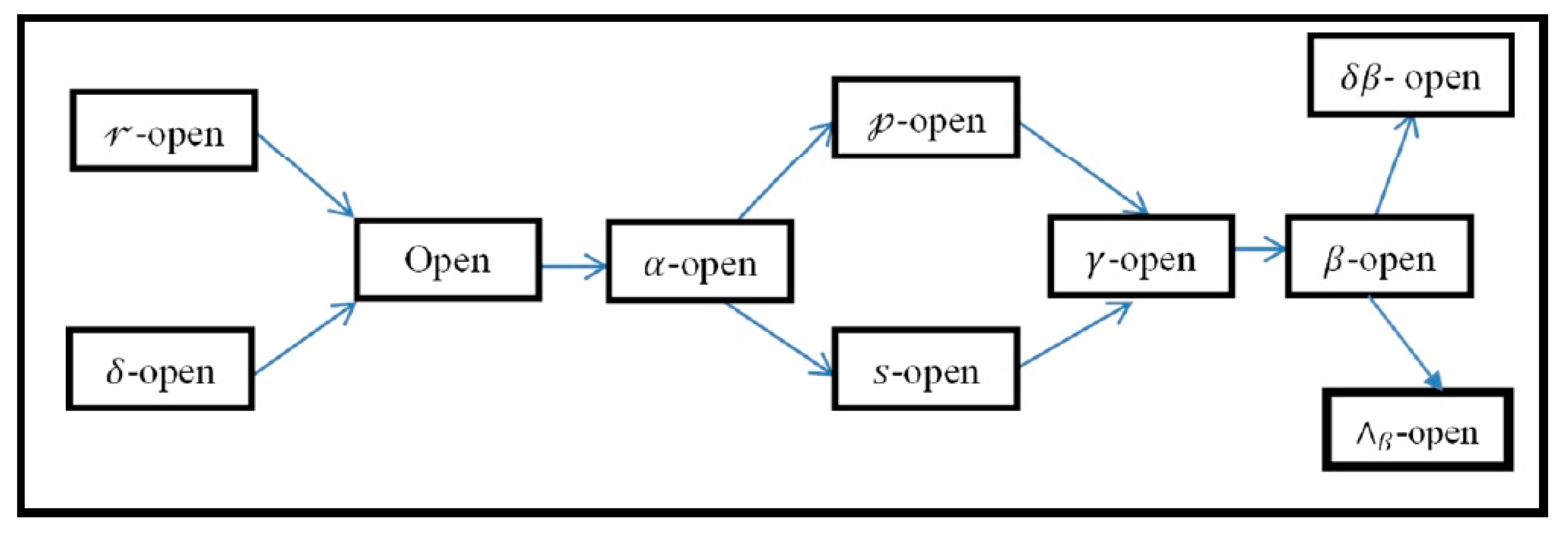
All the above-mentioned sets are called nearly open sets and the complements of these nearly open sets are called nearly closed sets. Moreover, the classes of all nearly open (resp. nearly closed) sets of $U$ denoted by $KO\left(U\right)$ (resp. $KC\left(U\right)$), for each $K\in \left\{𝓇, 𝓹, s, \gamma , \alpha , \beta ,\delta ,\delta \beta ,{\wedge }_{\beta }\right\}$

(ii) 

The relationship among different types of nearly open sets is given by Figure 1, and it is necessarily noticed that each arrow ($\to$) in the diagram represents a relation ($\subseteq$).

2.2. Rough Set Theory

Definition 7

[1]. The pair $\left(U,R\right)$ is named Pawlak approximation space (briefly, approximation space), such that $U$ represents a finite set and $R$ is an equivalence relation. For any $X\subseteq U$, the lower (resp. the upper) approximation of $X$ is given by $\underset{\_}{R}\left(X\right)=\left\{x\in X:{\left[x\right]}_R\subseteq X\right\}$ (resp. $\overline{R}\left(X\right)=\left\{x\in U:{\left[x\right]}_R{{\displaystyle \cap }}^{ }X\ne \varnothing \right\}$), where ${\left[x\right]}_R$ denotes an equivalence class in $R$ containing an element $x\in U$. According to [1], $X$ is called rough set if $\underset{\_}{R}\left(X\right)\ne \overline{R}\left(X\right)$.

Proposition 1

[1]. Let $X, Y \subseteq \left(U,R\right)$, Pawlak’s rough sets have the following properties:

(L1) $\underset{\_}{R}\left(X\right)\subseteq X$ (L2) $\underset{\_}{R}(\varnothing )=\varnothing$ (L3) $\underset{\_}{R}\left(U\right)=U$ (L4) $\underset{\_}{R}\left(X{{\displaystyle \cap }}^{ }Y\right)=\underset{\_}{R}\left(X\right){{\displaystyle \cap }}^{ }\underset{\_}{R}\left(Y\right)$  (L5) If $X\subseteq Y,$ then $\underset{\_}{R}\left(X\right)\subseteq \underset{\_}{R}\left(Y\right)$ (L6) $\underset{\_}{R}\left(X\right){{\displaystyle \cup }}^{ }\underset{\_}{R}\left(Y\right)\subseteq \underset{\_}{R}\left(X{{\displaystyle \cup }}^{ }Y\right)$ (L7) $\underset{\_}{R}\left(X^c\right)={(\overline{R}\left(X\right))}^c$ (L8) $\underset{\_}{R}\left(\underset{\_}{R}\left(X\right)\right)=\underset{\_}{R}\left(X\right)$ (L9) $\underset{\_}{R}\left({(\underset{\_}{R}\left(X\right))}^c\right)={(\underset{\_}{R}\left(X\right))}^c$ (L10) $\forall K\in U/R\Rightarrow \underset{\_}{R}\left(K\right)=K$

(U1) $X\subseteq \overline{R}\left(X\right)$ (U2) $\overline{R}(\varnothing )=\varnothing$ (U3) $\overline{R}\left(U\right)=U$ (U4) $\overline{R}\left(X{{\displaystyle \cup }}^{ }Y\right)=\overline{R}\left(X\right){{\displaystyle \cup }}^{ }\overline{R}\left(Y\right)$ (U5) If $X\subseteq Y,$ then $\overline{R}\left(X\right)\subseteq \overline{R}\left(Y\right)$ (U6) $\overline{R}\left(X\right){{\displaystyle \cap }}^{ }\overline{R}\left(Y\right)\supseteq \overline{R}\left(X{{\displaystyle \cap }}^{ }Y\right)$ (U7) $\overline{R}\left(X^c\right)={(\underset{\_}{R}\left(X\right))}^c$ (U8) $\overline{R}\left(\overline{R}\left(X\right)\right)=\overline{R}\left(X\right)$ (U9) $\overline{R}\left({(\overline{R}\left(X\right))}^c\right)={(\overline{R}\left(X\right))}^c$ (U10) $\forall K\in U/R \Rightarrow \overline{R}\left(K\right)=K$

To see the way to calculate Pawlak approximations, we give the next example.

Example 1.

Let $U=\left\{a,b,c,d\right\}$and $R=\{\left(a,a\right),\left(b,b\right),\left(c,c\right),\left(d,d\right),\left(a,b\right),\left(b,a\right)\}$. It is clear that $R$is an equivalence relation on $U$. Consider $X=\left\{a, c\right\}$and $Y=\left\{c, d\right\}$. Then, ${\left[a\right]}_R={\left[b\right]}_R=\left\{a, b\right\}$, ${\left[c\right]}_R=\left\{c\right\}$ and ${\left[d\right]}_R=\left\{d\right\}$. Therefore, $\underset{\_}{R}\left(X\right)=\left\{c\right\}$, $\overline{R}\left(X\right)=\left\{a,b,c\right\}$, and$\underset{\_}{R}\left(Y\right)=\overline{R}\left(Y\right)=\left\{c,d\right\}.$ Thus, $X$is a rough set, whereas $Y$is not a rough set. Obviously, $\underset{\_}{R}\left(X\right)=\left\{c\right\}\subset X=\left\{a,c\right\}\subset$$\overline{R}\left(X\right)=\left\{a,b,c\right\}$, also, $\underset{\_}{R}\left(X\right){{\displaystyle \cup }}^{ }\underset{\_}{R}\left(\left\{b\right\}\right)=\left\{c\right\}\subset \underset{\_}{R}\left(X{{\displaystyle \cup }}^{ }\left\{b\right\}\right)=\left\{a,b,c\right\}$ and $\overline{R}\left(X{{\displaystyle \cap }}^{ }Y\right)=\varnothing \subset \overline{R}\left(X\right){{\displaystyle \cap }}^{ }\overline{R}\left(Y\right)=\left\{c\right\}$.

2.3. j-Neighborhood Spaces

In this subsection, we present some important results and properties of the $j$-neighborhood space [10].

Definition 8

[10]. If $R$ is a binary relation on a non-empty finite set $U$, then the $j$-neighborhoods of $x\in U$ (denoted it by $N_j\left(x\right)$, $\forall j\in \left\{r, \ell , \langle r\rangle , \langle \ell \rangle , u, i, \langle u\rangle ,\langle i\rangle \right\}$) are defined by:

(i) 

$r$-neighborhood: $N_r\left(x\right)=\left\{y\in U: xRy\right\}$.

(ii) 

$\ell$-neighborhood: $N_{\ell }\left(x\right)=\left\{y\in U : yRx\right\}$.

(iii) 

$\langle r\rangle$-neighborhood: $N_{\langle r\rangle }\left(x\right)={{\displaystyle \cap }}_{x\in N_r\left(y\right)}{N}_r\left(y\right)$.

(iv) 

$\langle \ell \rangle$-neighborhood: $N_{\langle \ell \rangle }\left(x\right)={{\displaystyle \cap }}_{x\in N_{\ell }\left(y\right)}{N}_{\ell }\left(y\right)$.

(v) 

$i$-neighborhood: $N_i\left(x\right)=N_r\left(x\right){{\displaystyle \cap }}^{ }{N}_{\ell }\left(x\right)$.

(vi) 

$u$-neighborhood: $N_u\left(x\right)=N_r\left(x\right){{\displaystyle \cup }}^{ }{N}_{\ell }\left(x\right)$.

(vii) 

$\langle i\rangle$-neighborhood: $N_{\langle i\rangle }\left(x\right)=N_{\langle r\rangle }\left(x\right){{\displaystyle \cap }}^{ }{N}_{\langle \ell \rangle }\left(x\right)$.

(viii) 

$\langle u\rangle$-neighborhood: $N_{\langle u\rangle }\left(x\right)=N_{\langle r\rangle }\left(x\right){{\displaystyle \cup }}^{ }{N}_{\langle \ell \rangle }\left(x\right)$.

Definition 9

[10]. If $R$ is any relation on $U$ and the map ${\xi }_j:U\to P\left(U\right)$ assigns for each $x$ in $U$ it’s $N_j\left(x\right)$ in $P\left(U\right)$. Then the triple $\left(U, R, {\xi }_j\right)$ is called a $j$-NS.

Theorem 1

[10]. If $\left(U, R, {\xi }_j\right)$ is a $j$-NS, then for each $j\in \left\{r, \ell , \langle r\rangle , \langle \ell \rangle , u, i, \langle u\rangle ,\langle i\rangle \right\}$ the collection ${\tau }_j=\left\{A\subseteq U: \forall p\in A, N_j\left(p\right)\subseteq A \right\}$ is a topology on $U$.

Proposition 2

[10]. If $\left(U, R, {\xi }_j\right)$ is a $j$-NS, then ${\tau }_r$ represents a dual topology of ${\tau }_{\ell }$.

Proposition 3

[10]. Let $\left(U, R, {\xi }_j\right)$ be a $j$-NS. Then

$\left(i\right)$ ${\tau }_{u }\subseteq {\tau }_{r }\subseteq {\tau }_{i }$.	$\left(iii\right)$ ${\tau }_{\langle u\rangle }\subseteq {\tau }_{\langle r\rangle }\subseteq {\tau }_{\langle i\rangle }$.
$\left(ii\right)$ ${\tau }_{u }\subseteq {\tau }_{\ell }\subseteq {\tau }_{i }$.	$\left(iv\right)$ ${\tau }_{\langle u\rangle }\subseteq {\tau }_{\langle \ell \rangle }\subseteq {\tau }_{\langle i\rangle }$.

Definition 10

[10]. Consider $\left(U, R, {\xi }_j\right)$ to be a $j$-NS. Thus, a subset $A\subseteq U$ is called $j$-open set if $A\in {\tau }_j$, and its complement is called $j$-closed set. A class ${\Gamma }_j$ of all $j$-closed sets of a $j$-neighborhood space is given by ${\Gamma }_j=\{F\subseteq U | F^c \in {\tau }_j\}$, where $F^c$ means a complement of $F$.

Definition 11

[10]. Consider $\left(U, R, {\xi }_j\right)$ to be a $j$-NS and $A\subseteq U$. For each: $j\in \left\{r, \ell , \langle r\rangle , \langle \ell \rangle , u, i, \langle u\rangle ,\langle i\rangle \right\}$, the $j$-upper (resp. $j$-lower) approximation of $A$ is given by 

$${\overline{R}}_j\left(A\right)={{\displaystyle \cap }}^{ }\left\{H\in {\Gamma }_j:A\subseteq H\right\}=c{l}_j\left(A\right) (\mathrm{resp}. {\underset{\_}{R}}_j\left(A\right)={{\displaystyle \cup }}^{ }\left\{G\in {\tau }_j:G\subseteq A\right\}=in{t}_j\left(A\right)).$$

where, $c{l}_j\left(A\right)$ (resp. $in{t}_j\left(A\right)$) represents the $j$-closure of $A$ (resp. $j$-interior of $A$).

Definition 12

[10]. Let $j\in \left\{r, \ell , \langle r\rangle , \langle \ell \rangle , u, i, \langle u\rangle ,\langle i\rangle \right\}$, then a subset $A$ of a $j$-NS $\left(U, R, {\xi }_j\right)$called a $j$-exact set if ${\underset{\_}{R}}_j\left(A\right)={\overline{R}}_j\left(A\right)=A$. Otherwise, $A$ is called a $j$-rough set.

Definition 13

[10]. Consider $\left(U, R, {\xi }_j\right)$ to be a $j$-NS, and $A\subseteq U$. For each $j\in \left\{r, \ell , \langle r\rangle , \langle \ell \rangle , u, i, \langle u\rangle ,\langle i\rangle \right\}$, the $j$-positive, $j$-negative and $j$-boundary regions and $j$-accuracy of the approximations of $A\subseteq U$ are given by

$$PO{S}_j\left(A\right)={\underset{\_}{R}}_j\left(A\right), NE{G}_j\left(A\right)=U-{\overline{R}}_j\left(A\right),$$

$$B_j\left(A\right)={\overline{R}}_j\left(A\right)-{\underset{\_}{R}}_j\left(A\right) \mathrm{and} {\mu }_j\left(A\right)=\frac{\left|{\underset{\_}{R}}_j\left(A\right)\right|}{\left|{\overline{R}}_j\left(A\right)\right|} ,$$

respectively, where $\left|{\overline{R}}_j\left(A\right)\right|\ne 0$.

Obviously,$0\le {\mu }_j\left(A\right)\le 1$ and if ${\delta }_j\left(A\right)=1$, then $A$ is a $j$-exact set. Otherwise, it is a $j$-rough set.

Hosny [17] made use of the notions of $\delta \beta$-open sets and ${\wedge }_{\beta }$-open sets to establish two novel rough approximations which are two different generalizations of [10,12].

Definition 14

[17]. Let $\left(U, R,{\xi }_j\right)$ be a $j$-NS, $A\subseteq U$ and $j\in \left\{r, \ell , \langle r\rangle , \langle \ell \rangle , u, i, \langle u\rangle ,\langle i\rangle \right\}$. Then, a ${\delta }_j$-closure of  $A$ is defined by

$$c{l}_j^{\delta }\left(A\right)=\left\{x\in U:A{{\displaystyle \cap }}^{ }in{t}_j \left(c{l}_j\left(G\right)\right)\ne \varnothing , x\in G\in {\tau }_j\right\}.$$

A set $A$ is called ${\delta }_j$-closed set if $A=c{l}_j^{\delta }\left(A\right)$. We called the complement of a ${\delta }_j$-closed set a ${\delta }_j$-open set.

Note that: $in{t}_j^{\delta }\left(A\right)=U-c{l}_j^{\delta }\left(U-A\right)$.

Definition 15

[17]. Let $\left(U,R,{\xi }_j\right)$ be a $j$-NS, $A\subseteq U$ and $j\in \left\{r, \ell , \langle r\rangle , \langle \ell \rangle , u, i, \langle u\rangle ,\langle i\rangle \right\}$. Then, a subset $A$ is called a $\delta {\beta }_j$-open set if $A\subseteq c{l}_j[in{t}_j \left(c{l}_j^{\delta }\left(A\right)\right)]$ and the complement of $\delta {\beta }_j$-open set is called $\delta {\beta }_j$-closed.

The classes of all $\delta {\beta }_j$-open and $\delta {\beta }_j$-closed sets are respectively denoted by $\delta {\beta }_j O\left(U\right)$ and $\delta {\beta }_j C\left(U\right)$.

Definition 16

[17]. Let $\left(U,R,{\xi }_j\right)$ be a $j$-NS and $A\subseteq U$. Then, for each $j\in \left\{r, \ell , \langle r\rangle , \langle \ell \rangle , u, i, \langle u\rangle ,\langle i\rangle \right\}$, the $\delta {\beta }_j$-upper, $\delta {\beta }_j$-lower approximations, $\delta {\beta }_j$-positive, $\delta {\beta }_j$-negative and $\delta {\beta }_j$-boundary regions and $\delta {\beta }_j$-accuracy of the approximations $A$ are given by:

$$\begin{array}{l}{\overline{R}}_j^{\delta \beta }\left(A\right)={{\displaystyle \cap }}^{ }\left\{H\in \delta {\beta }_{j}C\left(U\right):A\subseteq H\right\}=\delta {\beta }_j-\mathrm{closure} \mathrm{of} A,\\ {\underset{\_}{R}}_j^{\delta \beta }\left(A\right)={{\displaystyle \cup }}^{ }\left\{G\in \delta {\beta }_{j}O\left(U\right):G\subseteq A\right\}=\delta {\beta }_j-\mathrm{interior} \mathrm{of} A,\end{array}$$

$$\begin{array}{l}PO{S}_j^{\delta \beta }\left(A\right)={\underset{\_}{R}}_j^{\delta \beta }\left(A\right), NE{G}_j^{\delta \beta }\left(A\right)=U-{\overline{R}}_j^{\delta \beta }\left(A\right) \mathrm{and}\\ B_j^{\delta \beta }\left(A\right)={\overline{R}}_j^{\delta \beta }\left(A\right)-{\underset{\_}{R}}_j^{\delta \beta }\left(A\right)\\ {\sigma }_j^{\delta \beta }\left(A\right)=\frac{\left|{\underset{\_}{R}}_j^{\delta \beta }\left(A\right)\right|}{\left|{\overline{R}}_j^{\delta \beta }\left(A\right)\right|}\end{array}$$

, respectively, where $\left|{\overline{R}}_j^{\delta \beta }\left(A\right)\right|\ne \varnothing$.

Definition 17

[17]. Let $\left(U,R,{\xi }_j\right)$ be a $j$-NS, $A\subseteq U$ and $\forall j\in \left\{r, \ell , \langle r\rangle , \langle \ell \rangle , u, i, \langle u\rangle ,\langle i\rangle \right\}$. The subset ${\wedge }_{{\beta }_j} \left(A\right)$ is defined by ${\wedge }_{{\beta }_j} \left(A\right)={{\displaystyle \cap }}^{ }\left\{G\subseteq U:A\subseteq G,G\in {\beta }_{j}O\left(U\right)\right\}$.

A subset $A$ is said to be a ${\wedge }_{{\beta }_j}$-set if $A={\wedge }_{{\beta }_j}\left(A\right)$. The complement of a ${\wedge }_{{\beta }_j}$-set is called a ${\vee }_{{\beta }_j}$-set. The family of all ${\wedge }_{{\beta }_j}$-set and ${\vee }_{{\beta }_j}$ is denoted by ${\tau }_j^{{\wedge }_{\beta }}$ and ${\tau }_j^{{\vee }_{\beta }}$, respectively.

Definition 18

[17]. Let $\left(U,R,{\xi }_j\right)$ be a$j$-NS, $A\subseteq U$ and $\forall j\in \left\{r, \ell , \langle r\rangle , \langle \ell \rangle , u, i, \langle u\rangle ,\langle i\rangle \right\}$, The (${\wedge }_{{\beta }_j}$-upper, and ${\wedge }_{{\beta }_j}$-lower) approximations, (${\wedge }_{{\beta }_j}$-positive, ${\wedge }_{{\beta }_j}$-negative and ${\wedge }_{{\beta }_j}$-boundary) regions and the ${\wedge }_{{\beta }_j}$-accuracy of approximations of $A$ are given by:

$${\overline{R}}_j^{{\wedge }_{\beta }}\left(A\right)={{\displaystyle \cap }}^{ }\left\{H\in {\tau }_j^{{\vee }_{\beta }}:A\subseteq H\right\}={\vee }_{{\beta }_j}-\mathrm{closure} \mathrm{of} A,$$

$${\underset{\_}{R}}_j^{{\wedge }_{\beta }}\left(A\right)={{\displaystyle \cup }}^{ }\left\{G\in {\tau }_j^{{\wedge }_{\beta }}:G\subseteq A\right\}={\wedge }_{{\beta }_j}-\mathrm{interior} \mathrm{of} A,$$

$$\begin{array}{l}PO{S}_j^{{\wedge }_{\beta }}\left(A\right)={\underset{\_}{R}}_j^{{\wedge }_{\beta }}\left(A\right), NE{G}_j^{{\wedge }_{\beta }}\left(A\right)=U-{\overline{R}}_j^{{\wedge }_{\beta }}\left(A\right),\\ B_j^{{\wedge }_{\beta }}\left(A\right)={\overline{R}}_j^{{\wedge }_{\beta }}\left(A\right)-{\underset{\_}{R}}_j^{{\wedge }_{\beta }}\left(A\right) \mathrm{and} {\sigma }_j^{{\wedge }_{\beta }}\left(A\right)=\frac{\left|{\underset{\_}{R}}_j^{{\wedge }_{\beta }}\left(A\right)\right|}{\left|{\overline{R}}_j^{{\wedge }_{\beta }}\left(A\right)\right|}, \\ \mathrm{respectively}, \mathrm{where} \left|{\overline{R}}_j^{{\wedge }_{\beta }}\left(A\right)\right|\ne \varnothing .\end{array}$$

The above rough approximations are given more detailed treatment in previous studies [12,17].

3. Generalized j-Neighborhood Spaces and j-Adhesion Approximations

In this portion, we study further properties of the concepts of $j$-adhesion neighborhoods and show the relationships among them with the aid of some examples. Then, we discuss two methods to induce different topologies using $j$-adhesion neighborhoods. One of the interesting results states that those topologies are quasi-discrete. Finally, we initiate some approximations using $j$-adhesion neighborhoods.

3.1. Further Properties and Relationships among j-Neighborhoods Spaces and j-Adhesion Neighborhoods

Definition 19

[9,37,39]. Let $\left(U, R,{\xi }_j\right)$ be a $j$-NS. Then, we define the $j$-adhesion neighborhoods $P_j\left(t\right)$ of$t\in U$, such that $j\in \left\{r, \ell , \langle r\rangle , \langle \ell \rangle , u, i, \langle u\rangle ,\langle i\rangle \right\}$), are

(i) 

$P_r\left(t\right)=\left\{s\in U : N_r\left(s\right)=N_r\left(t\right)\right\}$.

(ii) 

$P_{\ell }\left(t\right)=\left\{s\in U : N_{\ell }\left(s\right)=N_{\ell }\left(t\right)\right\}$.

(iii) 

$P_i\left(t\right)=P_r\left(t\right){{\displaystyle \cap }}^{ }{P}_{\ell }\left(t\right)$.

(iv) 

$P_u\left(t\right)=P_r\left(t\right){{\displaystyle \cup }}^{ }{P}_{\ell }\left(t\right)$.

(v) 

$P_{\langle r\rangle }\left(t\right)=\left\{s\in U :N_{\langle r\rangle }\left(s\right)=N_{\langle r\rangle }\left(t\right)\right\}$.

(vi) 

$P_{\langle \ell \rangle }\left(t\right)=\left\{s\in U : N_{\langle \ell \rangle }\left(s\right)=N_{\langle \ell \rangle }\left(t\right)\right\}$.

(vii) 

$P_{\langle i\rangle }\left(t\right)=P_{\langle r\rangle }\left(t\right){{\displaystyle \cap }}^{ }{P}_{\langle \ell \rangle }\left(t\right)$.

(viii) 

$P_{\langle u\rangle }\left(t\right)=P_{\langle r\rangle }\left(t\right){{\displaystyle \cup }}^{ }{P}_{\langle \ell \rangle }\left(t\right)$.

We give the next example to see the way of calculating them.

Example 2.

Let$U=\left\{a,b,c,d\right\}$and$R=\{\left(c,a\right),\left(d,a\right),\left(c,b\right),$$\left(d,c\right),\left(c,d\right),\left(d,d\right)\}$.Then, we get the

Table 1. The $j$-neighborhoods of $x\in U$.

$\mathit{x}\in \mathit{U}$	$\mathit{a}$	$\mathit{b}$	$\mathit{c}$	$\mathit{d}$
$N_r\left(x\right)$	$\varnothing$	$\varnothing$	$\left\{a,b,d\right\}$	$\left\{a,c,d\right\}$
$N_{\ell }\left(x\right)$	$\left\{c,d\right\}$	$\left\{c\right\}$	$\left\{d\right\}$	$\left\{c,d\right\}$
$N_i\left(x\right)$	$\varnothing$	$\varnothing$	$\left\{d\right\}$	$\left\{c,d\right\}$
$N_u\left(x\right)$	$\left\{c,d\right\}$	$\left\{c\right\}$	$\left\{a,b,d\right\}$	$\left\{a,c,d\right\}$
$N_{\langle r\rangle }\left(x\right)$	$\left\{a,d\right\}$	$\left\{a,b,d\right\}$	$\left\{a,c,d\right\}$	$\left\{a,d\right\}$
$N_{\langle \ell \rangle }\left(x\right)$	$\varnothing$	$\varnothing$	$\left\{c\right\}$	$\left\{d\right\}$
$N_{\langle i\rangle }\left(x\right)$	$\varnothing$	$\varnothing$	$\left\{c\right\}$	$\left\{d\right\}$
$N_{\langle u\rangle }\left(x\right)$	$\left\{a,d\right\}$	$\left\{a,b,d\right\}$	$\left\{a,c,d\right\}$	$\left\{a,d\right\}$

and

Table 2. The $j$-adhesion neighborhoods of $x\in U$.

$\mathit{x}\in \mathit{U}$	$\mathit{a}$	$\mathit{b}$	$\mathit{c}$	$\mathit{d}$
$P_r\left(x\right)$	$\left\{a,b\right\}$	$\left\{a,b\right\}$	$\left\{c\right\}$	$\left\{d\right\}$
$P_{\ell }\left(x\right)$	$\left\{a,d\right\}$	$\left\{b\right\}$	$\left\{c\right\}$	$\left\{a,d\right\}$
$P_i\left(x\right)$	$\left\{a\right\}$	$\left\{b\right\}$	$\left\{c\right\}$	$\left\{d\right\}$
$P_u\left(x\right)$	$\left\{a,b,d\right\}$	$\left\{a,b\right\}$	$\left\{c\right\}$	$\left\{a,d\right\}$
$P_{\langle r\rangle }\left(x\right)$	$\left\{a,d\right\}$	$\left\{b\right\}$	$\left\{c\right\}$	$\left\{a,d\right\}$
$P_{\langle \ell \rangle }\left(x\right)$	$\left\{a,b\right\}$	$\left\{a,b\right\}$	$\left\{c\right\}$	$\left\{d\right\}$
$p_{\langle i\rangle }\left(x\right)$	$\left\{a\right\}$	$\left\{b\right\}$	$\left\{c\right\}$	$\left\{d\right\}$
$P_{\langle u\rangle }\left(x\right)$	$\left\{a,b,d\right\}$	$\left\{a,b\right\}$	$\left\{c\right\}$	$\left\{a,d\right\}$

.

In what follows, we list the basic properties of the concepts of $j$-adhesion neighborhoods.

We begin with the next result which is a direct observation of Definition 19.

Proposition 4.

Let$\left(U, R,{\xi }_j\right)$be a$j$-NS and$\forall j\in \left\{r, \ell , \langle r\rangle , \langle \ell \rangle , u, i, \langle u\rangle ,\langle i\rangle \right\}$. Then, $\forall x\in U$:

(i) 

$P_i\left(x\right)\subseteq P_r\left(x\right)\subseteq P_u\left(x\right)$.

(ii) 

$P_i\left(x\right)\subseteq P_{\ell }\left(x\right)\subseteq P_u\left(x\right)$.

(iii) 

$P_{\langle i\rangle }\left(x\right)\subseteq P_{\langle r\rangle }\left(x\right)\subseteq P_{\langle u\rangle }\left(x\right)$.

(iv) 

$P_{\langle i\rangle }\left(x\right)\subseteq P_{\langle \ell \rangle }\left(x\right)\subseteq P_{\langle u\rangle }\left(x\right)$.

Proposition 5.

Let$\left(U, R,{\xi }_j\right)$be a$j$-NS and $j\in \left\{r, \ell , \langle r\rangle , \langle \ell \rangle , i, \langle i\rangle \right\}$. Then: 

(i) 

For each$x\in U$: $x\in P_j\left(x\right)$.

(ii) 

$y\in P_j\left(x\right)$if and only if$P_j\left(y\right)=P_j\left(x\right)$.

Proof 

. The first statement (i) is obvious from Definition 19. So, we only prove (ii) in the case of $j=r$. The further cases can be made by similar way.

$$\mathrm{First}, \mathrm{let} y\in P_r\left(x\right). \mathrm{Then} N_r\left(y\right)=N_r\left(x\right)$$

Let $z\in P_r\left(y\right)$, then $N_r\left(z\right)=N_r\left(y\right)$. By (1), we get $N_r\left(z\right)=N_r\left(x\right)$. This means that $z\in P_r\left(x\right)$. Thus, $P_r\left(y\right)\subseteq P_r\left(x\right)$. Similarly, one can prove that $P_r\left(y\right)\supseteq P_r\left(x\right)$.

In Example 2, note that $a\in P_u\left(b\right)$. But $P_u\left(a\right)\not\subset P_u\left(b\right)$. Also, $a\in P_{\langle u\rangle }\left(b\right)$. But $P_{\langle u\rangle }\left(a\right)\not\subset P_{\langle u\rangle }\left(b\right)$. Hence, the above proposition does not hold in the cases of $j\in \left\{u, \langle u\rangle \right\}$. □

Corollary 1. 

Let $\left(U, R,{\xi }_j\right)$ be a $j$-NS, $X,Y\subseteq U$ and $\forall j\in \left\{r, \ell , \langle r\rangle , \langle \ell \rangle , i, \langle i\rangle \right\}$. Then, the class ${\wp }_j\left(U\right)=\{P_j\left(x\right):x\in U\}$forms a partition on $U$.

Note that in Example 2 we can get ${\wp }_u\left(U\right)=\left\{\left\{c\right\},\left\{a,b\right\},\left\{a,d\right\},\left\{a,b,d\right\}\right\}$. Obviously, $\left\{a,b\right\}{{\displaystyle \cap }}^{ }\left\{a,d\right\}=\left\{a\right\}\ne \varnothing$ and $\left\{a,d\right\}{{\displaystyle \cap }}^{ }\left\{a,b,d\right\}=\left\{a,d\right\}\ne \varnothing$ and this means that ${\wp }_u\left(U\right)$ is not a partition on $U$. Hence, the class ${\wp }_j\left(U\right)$ need not be a partition on $U$ in the cases of $j\in \left\{ u, \langle u\rangle \right\}$.

Proposition 6.

Let $\left(U, R,{\xi }_j\right)$ be a $j$-NS. Then, foreach $x\in U:$

(i) 

$P_{\langle r\rangle }\left(x\right)=P_{\ell }\left(x\right)$.

(ii) 

$P_{\langle \ell \rangle }\left(x\right)=P_r\left(x\right)$.

Proof. 

Only, the first statement will be proved and the other can be made similarly.

Let $y\in P_{\langle r\rangle }\left(x\right)$. Then $P_{\langle r\rangle }\left(y\right)=P_{\langle r\rangle }\left(x\right)$ and $N_{\langle r\rangle }\left(x\right)=N_{\langle r\rangle }\left(y\right)$ … (1).

Now, we must prove that $P_{\ell }\left(y\right)=P_{\ell }\left(x\right)$ as follows:

Assume that $P_{\ell }\left(y\right)\ne P_{\ell }\left(x\right)$, then $y\notin P_{\ell }\left(x\right)$ and $x\notin P_{\ell }\left(y\right)$. Hence, $N_{\ell }\left(x\right)\ne N_{\ell }\left(y\right)$ and this means that $\exists z\in N_{\ell }\left(y\right)$ such that $z\notin N_{\ell }\left(x\right)$. Accordingly, $y\in N_r\left(z\right)$ and $x\notin N_r\left(z\right)$ which implies $z\in N_{\langle r\rangle }\left(y\right)$ and $z\notin N_{\langle r\rangle }\left(x\right)$. Therefore, $N_{\langle r\rangle }\left(x\right)\ne N_{\langle r\rangle }\left(y\right)$ and this contradicts assumption (1).

Hence, $y\in P_{\ell }\left(x\right)$ and this implies $P_{\langle r\rangle }\left(x\right)\subseteq P_{\ell }\left(x\right)$.

Conversely, by using similar arguments, we can prove $P_{\langle r\rangle }\left(x\right)\supseteq P_{\ell }\left(x\right)$.

Following similar arguments, one can prove (ii). □

Corollary 2.

Let $\left(U, R,{\xi }_j\right)$ be a $j$-NS. Then, for each $x\in U:$

(i) 

$P_{\langle i\rangle }\left(x\right)=P_i\left(x\right)$.

(ii) 

$P_{\langle u\rangle }\left(x\right)=P_u\left(x\right)$.

Proof. 

By using Proposition 6., we obtain:

$$P_i\left(x\right)=P_r\left(x\right){{\displaystyle \cap }}^{ }{P}_{\ell }\left(x\right)=P_{\langle \ell \rangle }\left(x\right){{\displaystyle \cap }}^{ }{P}_{\langle r\rangle }\left(x\right)=P_{\langle i\rangle }\left(x\right).$$

By similar way, we can prove $P_{\langle u\rangle }\left(x\right)=P_u\left(x\right).$ □

Note that from Proposition 6 and Corollary 2, for any $j$-NS we can generate four different $j$-adhesion neighborhoods via a binary relation although we get eight different $j$-neighborhoods from the same relation.

We investigate in the following results some properties of the $j$-adhesion neighborhoods and $j$-neighborhoods and the interrelations between them with respect to some types of the relation $R$.

Proposition 7.

Consider $\left(U, R,{\xi }_j\right)$ to be a $j$-NS, $x\in U$ and for each $j\in \left\{r, \ell , \langle r\rangle , \langle \ell \rangle , u, i, \langle u\rangle ,\langle i\rangle \right\}$. If$R$is a reflexive relation on $U$, then:

1. 

$N_j\left(x\right)\ne \varnothing , \forall x\in U$.

2. 

$x\in N_j\left(x\right), \forall x\in U$.

3. 

$P_j\left(x\right)\subseteq N_j\left(x\right), \forall x\in U$.

Proof. 

We only prove (iii) when $j=r$. The other cases can be made similarly.

Let $y\in P_r\left(x\right)$, then $N_r\left(y\right)=N_r\left(x\right)$. Since $R$ is a reflexive relation on $U$, then $y\in N_r\left(y\right)$. This implies that $y\in N_r\left(x\right)$. Hence, $P_j\left(x\right)\subseteq N_j\left(x\right), \forall x\in U$. □

To show that the converse of (iii) of Proposition 7 need not be true, we present the next example.

Example 3. 

If $U=\left\{a,b,c,d\right\}$ and $R=\left\{\left(a,a\right),\left(a,b\right),\left(b,b\right),\left(c,c\right),\left(c,a\right),\left(d,d\right)\right\}$. Then, we get the following

Table 3. The $j$-neighborhoods of $x\in U$.

$\mathit{x}\in \mathit{U}$	$\mathit{a}$	$\mathit{b}$	$\mathit{c}$
$N_r\left(x\right)$	$\left\{a,b\right\}$	$\left\{b\right\}$	$\left\{a,c\right\}$
$N_{\ell }\left(x\right)$	$\left\{a,c\right\}$	$\left\{a,b\right\}$	$\left\{c\right\}$
$N_i\left(x\right)$	$\left\{a\right\}$	$\left\{b\right\}$	$\left\{c\right\}$
$N_u\left(x\right)$	$\left\{a,b,c\right\}$	$\left\{a,b\right\}$	$\left\{a,c\right\}$
$N_{\langle r\rangle }\left(x\right)$	$\left\{a\right\}$	$\left\{b\right\}$.	$\left\{a,c\right\}$
$N_{\langle \ell \rangle }\left(x\right)$	$\left\{a\right\}$	$\left\{a,b\right\}$	$\left\{c\right\}$
$N_{\langle i\rangle }\left(x\right)$	$\left\{a\right\}$	$\left\{b\right\}$	$\left\{c\right\}$
$N_{\langle u\rangle }\left(x\right)$	$\left\{a\right\}$	$\left\{a,b\right\}$	$\left\{a,c\right\}$

and

Table 4. The $j$-adhesion neighborhoods of $x\in U$.

$\mathit{x}\in \mathit{U}$	$\mathit{a}$	$\mathit{b}$	$\mathit{c}$
$P_r\left(x\right)$	$\left\{a\right\}$	$\left\{b\right\}$	$\left\{c\right\}$
$P_{\ell }\left(x\right)$	$\left\{a\right\}$	$\left\{b\right\}$	$\left\{c\right\}$
$P_i\left(x\right)$	$\left\{a\right\}$	$\left\{b\right\}$	$\left\{c\right\}$
$P_u\left(x\right)$	$\left\{a\right\}$	$\left\{b\right\}$	$\left\{c\right\}$
$P_{\langle r\rangle }\left(x\right)$	$\left\{a\right\}$	$\left\{b\right\}$	$\left\{c\right\}$
$P_{\langle \ell \rangle }\left(x\right)$	$\left\{a\right\}$	$\left\{b\right\}$	$\left\{c\right\}$
$p_{\langle i\rangle }\left(x\right)$	$\left\{a\right\}$	$\left\{b\right\}$	$\left\{c\right\}$
$P_{\langle u\rangle }\left(x\right)$	$\left\{a\right\}$	$\left\{b\right\}$	$\left\{c\right\}$

.

Proposition 8.

Consider$\left(U, R,{\xi }_j\right)$ to be a $j$-NS. If$R$ is a reflexive relation on $U$, then $\forall x\in U$:

• $N_{\langle r\rangle }\left(x\right)\subseteq N_r\left(x\right)$.
• $N_{\langle \ell \rangle }\left(x\right)\subseteq N_{\ell }\left(x\right)$.
• $N_{\langle i\rangle }\left(x\right)\subseteq N_i\left(x\right)$.
• $N_{\langle u\rangle }\left(x\right)\subseteq N_u\left(x\right)$.

Proof. 

We only prove (i). The other cases follow similar lines.

Let $y\in N_{\langle r\rangle }\left(x\right)$. Then for each $z\in U$ such that $zRx$ we have $y\in N_r\left(z\right)$. Since $R$ is a reflexive relation on $U$, then $x\in N_r\left(x\right)$. Therefore $y\in N_r\left(x\right)$. Hence, we obtain the desired result. □

Example 3 illustrates that the converse of Proposition 8 fails.

Lemma 1.

Let$\left(U, R,{\xi }_j\right)$ be a$j$-NS and$R$be a symmetric relation. Then, $\forall x\in U$:

• $N_r\left(x\right)=N_{\ell }\left(x\right)=N_i\left(x\right)=N_u\left(x\right)$.
• $N_{\langle r\rangle }\left(x\right)=N_{\langle \ell \rangle }\left(x\right)=N_{\langle i\rangle }\left(x\right)=N_{\langle u\rangle }\left(x\right)$.

Proof. 

To prove (i), let $R$ be a symmetric relation. Then $xRy\iff yRx$ and this means that $y\in N_r\left(x\right)\iff y\in N_{\ell }\left(x\right)$. Thus $N_r\left(x\right)=N_{\ell }\left(x\right)$ and this implies:

$$N_r\left(x\right)=N_{\ell }\left(x\right)=N_i\left(x\right)=N_u\left(x\right).$$

Following similar arguments, one can prove (ii). □

Corollary 3.

Consider$\left(U, R,{\xi }_j\right)$ to be a$j$-NS, $\forall x\in U$ and for every $j\in \left\{r, \ell , \langle r\rangle , \langle \ell \rangle , u, i, \langle u\rangle ,\langle i\rangle \right\}$. If$R$is a symmetric relation, then all$j$-adhesion neighborhoods are identical. That is, for each$x\in U$: $P_r\left(x\right)=P_{\ell }\left(x\right)=P_i\left(x\right)=P_u\left(x\right)=P_{\langle r\rangle }\left(x\right)=P_{\langle \ell \rangle }\left(x\right)=P_{\langle i\rangle }\left(x\right)=P_{\langle u\rangle }\left(x\right)$.

Example 4.

Let$U=\left\{a,b,c,d\right\}$ and$R=\left\{\left(a,b\right),\left(a,c\right),\left(b,a\right),\left(b,b\right), \left(c,a\right)\right\}$. Then, we get 

Table 5. The $j$-neighborhoods of $x\in U$.

$\mathit{x}\in \mathit{U}$	$\mathit{a}$	$\mathit{b}$	$\mathit{c}$
$N_r\left(x\right)$	$\left\{b,c\right\}$	$\left\{a,b\right\}$	$\left\{a\right\}$
$N_{\ell }\left(x\right)$	$\left\{b,c\right\}$	$\left\{a,b\right\}$	$\left\{a\right\}$
$N_i\left(x\right)$	$\left\{b,c\right\}$	$\left\{a,b\right\}$	$\left\{a\right\}$
$N_u\left(x\right)$	$\left\{b,c\right\}$	$\left\{a,b\right\}$	$\left\{a\right\}$
$N_{\langle r\rangle }\left(x\right)$	$\left\{a\right\}$	$\left\{b\right\}$	$\left\{b,c\right\}$
$N_{\langle \ell \rangle }\left(x\right)$	$\left\{a\right\}$	$\left\{b\right\}$	$\left\{b,c\right\}$
$N_{\langle i\rangle }\left(x\right)$	$\left\{a\right\}$	$\left\{b\right\}$	$\left\{b,c\right\}$
$N_{\langle u\rangle }\left(x\right)$	$\left\{a\right\}$	$\left\{b\right\}$	$\left\{b,c\right\}$

and 

Table 6. The $j$-adhesion neighborhoods of $x\in U$.

$\mathit{x}\in \mathit{U}$	$\mathit{a}$	$\mathit{b}$	$\mathit{c}$
$P_r\left(x\right)$	$\left\{a\right\}$	$\left\{b\right\}$	$\left\{c\right\}$
$P_{\ell }\left(x\right)$	$\left\{a\right\}$	$\left\{b\right\}$	$\left\{c\right\}$
$P_i\left(x\right)$	$\left\{a\right\}$	$\left\{b\right\}$	$\left\{c\right\}$
$P_u\left(x\right)$	$\left\{a\right\}$	$\left\{b\right\}$	$\left\{c\right\}$
$P_{\langle r\rangle }\left(x\right)$	$\left\{a\right\}$	$\left\{b\right\}$	$\left\{c\right\}$
$P_{\langle \ell \rangle }\left(x\right)$	$\left\{a\right\}$	$\left\{b\right\}$	$\left\{c\right\}$
$p_{\langle i\rangle }\left(x\right)$	$\left\{a\right\}$	$\left\{b\right\}$	$\left\{c\right\}$
$P_{\langle u\rangle }\left(x\right)$	$\left\{a\right\}$	$\left\{b\right\}$	$\left\{c\right\}$

.

3.2. Topologies Generated by $j$-Adhesion Neighborhoods

Theorem 2.

If $\left(U,R,{\xi }_j\right)$ is a$j$-NS, then for each $j\in \left\{r,\ell ,\langle r\rangle ,\langle \ell \rangle ,u,i,\langle u\rangle ,\langle i\rangle \right\}$ the collection ${\mathcal{T}}_{P_j}=\left\{A\subseteq U:\forall x\in A,P_j\left(x\right)\subseteq A\right\}$ is a topology on $U$.

Proof. 

Using Theorem 1, the proof is obvious. □

Proposition 9.

Let$\left(U,R,{\xi }_j\right)$ be a$j$-NS and $\forall j\in \left\{r,\ell ,\langle r\rangle ,\langle \ell \rangle ,i,\langle i\rangle \right\}$. Then the topologies${\mathcal{T}}_{P_j}$ are quasi-discrete.

Proof. 

Since, for each $j\in \left\{r,\ell ,\langle r\rangle ,\langle \ell \rangle ,i,\langle i\rangle \right\}$, the families ${\wp }_j\left(U\right)=\{P_j\left(x\right):x\in U\}$ forms a partition on $U$ (Corollary 1). Then the topologies ${\mathcal{T}}_{P_j}$ are quasi-discrete. □

Note that For any $j\in \left\{u,\langle u\rangle \right\}$ in a $j$-NS, the topologies ${\mathcal{T}}_{P_j}$ need not be a quasi-discrete in general as Example 2 illustrated.

Remark 2.

Let$\left(U,R,{\xi }_j\right)$ be a$j$-NS. Then the topology ${\mathcal{T}}_{P_r}$ need not be the dual topology to${\mathcal{T}}_{P_{\ell }}$ (although ${\tau }_{r }$ and${\tau }_{\ell }$are dual topologies, see Proposition 1 [10]) as shown in the next example.

Example 5.

According to Example 2, we get:

$${\mathcal{T}}_{P_r}=\left\{U,\varnothing ,\left\{c\right\},\left\{d\right\},\left\{a,b\right\},\left\{c,d\right\},\left\{a,b,c\right\},\left\{a,b,d\right\}\right\} \mathrm{and}$$

$${\mathcal{T}}_{P_{\ell }}=\left\{U,\varnothing ,\left\{b\right\},\left\{c\right\},\left\{a,d\right\},\left\{b,c\right\},\left\{a,b,d\right\},\left\{a,c,d\right\}\right\}.$$

It is clear that ${\mathcal{T}}_{P_r}$ and${\mathcal{T}}_{P_{\ell }}$ are not comparable.

Proposition 10.

Let$\left(U,R,{\xi }_j\right)$ be a$j$-NS. Then

$\left(i\right)$

${\mathcal{T}}_{P_u}\subseteq {\mathcal{T}}_{P_r}\subseteq {\mathcal{T}}_{P_i}$.

$\left(ii\right)$

${\mathcal{T}}_{P_u}\subseteq {\mathcal{T}}_{P_{\ell }}\subseteq {\mathcal{T}}_{P_i}$.

$\left(iii\right)$

${\mathcal{T}}_{P_{\left(u\right)}}\subseteq {\mathcal{T}}_{P_{\left(r\right)}}\subseteq {\mathcal{T}}_{P_{\left(i\right)}}$.

$\left(iv\right)$

${\mathcal{T}}_{P_{\left(u\right)}}\subseteq {\mathcal{T}}_{P_{(\ell )}}\subseteq {\mathcal{T}}_{P_{\left(i\right)}}$.

Proof. 

Directly from Proposition 4. □

Proposition 11.

Let$\left(U,R,{\xi }_j\right)$ be a$j$-NS. Then

$\left(i\right)$

${\mathcal{T}}_{P_r}={\mathcal{T}}_{P_{(\ell )}}$and${\mathcal{T}}_{P_{\ell }}={\mathcal{T}}_{P_{\left(r\right)}}$

$\left(ii\right)$

${\mathcal{T}}_{P_i}={\mathcal{T}}_{P_{\left(i\right)}}$and${\mathcal{T}}_{P_u}={\mathcal{T}}_{P_{\left(u\right)}}$.

Proof. 

From Proposition 6, the proof holds. □

The essential target of the following result is to give the relationships between the topologies ${\tau }_j$, generated by $j$-neighborhoods, and the topologies ${\mathcal{T}}_{P_j}$, generated by $j$-adhesion neighborhoods.

Proposition 12.

Let$\left(U,R,{\xi }_j\right)$ be a$j$-NS and$R$be a reflexive relation. Then, for each$j\in \left\{r,\ell ,\langle r\rangle ,\langle \ell \rangle ,u,i,\langle u\rangle ,\langle i\rangle \right\}$: ${\tau }_j\subseteq {\mathcal{T}}_{P_j}$.

Proof. 

According to Proposition 7, the proof is clear. □

Example below illustrates that the reflexivity condition is necessary in the above proposition.

Example 6.

Consider Example 2, we illustrate the topologies${\tau }_j$ and${\mathcal{T}}_{P_j}$ are not comparable, in general, for the case of $j=r$ and the others similarly as follows:

$${\tau }_r=\left\{U,\varnothing ,\left\{a\right\},\left\{b\right\},\left\{a,b\right\}\right\} \mathrm{and} {\mathcal{T}}_{P_r}=\left\{U,\varnothing ,\left\{c\right\},\left\{d\right\},\left\{a,b\right\},\left\{c,d\right\},\left\{a,b,c\right\},\left\{a,b,d\right\}\right\}.$$

Definition 20.

Let$\left(U,R,{\xi }_j\right)$ be a$j$-NS and $\forall j\in \left\{r,\ell ,\langle r\rangle ,\langle \ell \rangle ,u,i,\langle u\rangle ,\langle i\rangle \right\}$. Thus, a subset $X\subseteq U$ is called$j$-adhesion open set if $X\in {\mathcal{T}}_{P_j}$, and the complement of a$j$-adhesion open set is said to be$j$-adhesion closed set. The class${ℱ}_{P_j}$of all$j$-adhesion closed sets is given by:

$${ℱ}_{P_j}=\left\{F\subseteq U|F^c\in {\mathcal{T}}_{P_j}\right\}.$$

Definition 21.

Let$\left(U,R,{\xi }_j\right)$ be a$j$-NS, $X\subseteq U$ and$\forall j\in \left\{r,\ell ,\langle r\rangle ,\langle \ell \rangle ,i,\langle i\rangle \right\}$. The$j$-adhesion interior (resp.$j$-adhesion closure) of$X$, that given by a topological space ${\mathcal{T}}_{P_j}$, is defined by${\mathit{int}}_j^{\mathcal{P}}(X)=\cup \{G\in {\mathcal{T}}_{P_j}:G\subseteq X\}$ (resp. ${\mathit{cl}}_j^{\mathcal{P}}(A)=\cap \{H\in {\mathcal{F}}_{P_j}:X\subseteq H\}$).

3.3. Generalized Rough Approximations Based on j-Adhesion Neighborhoods

In the present subsection, we discuss a topological view to $j$-adhesion rough sets that are given in related studies [9,37,39] and give some more properties of them.

Definition 22. Let$\left(U, R,{\xi }_j\right)$ be a$j$-NSand${\mathcal{T}}_{P_j}$ be a topology generated by$j$-adhesion neighborhoods. Then for every$A\subseteq U$ and$\in \{r, \ell , \langle r\rangle , \langle \ell \rangle ,$ $u, i, \langle u\rangle ,\langle i\rangle \}$, the$j$-adhesion (upper, and lower) approximations,$j$-adhesion (boundary, positive, and negative) regions and the$j$-adhesion accuracy of$j$-adhesion approximations of$A$are given by

$${\overline{\mathcal{P}}}_j(X)=\cap \{H\in {\mathcal{F}}_{P_j}:X\subseteq H\}=c{l}_j^{\mathcal{P}}(X),$$

$${\underset{¯}{\mathcal{P}}}_j(X)=\cup \{G\in {\mathcal{J}}_{P_j}:G\subseteq X\}=in{t}_j^{\mathcal{P}}(X),$$

$${\mathcal{B}}_{P_j}(X)={\overline{\mathcal{P}}}_j(X)-{\underset{\_}{\mathcal{P}}}_j(X),$$

$$PO{S}_{P_j}(X)={\underset{\_}{\mathcal{P}}}_j(X),$$

$$NE{G}_{P_j}(X)=U-{\stackrel{\_}{\mathcal{P}}}_j(X), \mathrm{and}$$

$${\rho }_{P_j}(X)=\frac{|{\underset{\_}{\mathcal{P}}}_j(X)|}{|{\overline{\mathcal{P}}}_j(X)|}, \mathrm{respectively}, \mathrm{where} |{\overline{\mathcal{P}}}_j(X)|\ne 0.$$

It is clear that: $0\le {\rho }_{P_j}\left(X\right)\le 1$.

The next propositions demonstrate the main properties of $\mathrm{j}$-adhesion approximations.

Proposition 13.

Let$\left(U, R,{\xi }_j\right)$ be a$j$-NS, and${\mathcal{T}}_{P_j}$ be a topology that generated by$j$-adhesion neighborhoods. Then, for every$X\subseteq U$ and$\in \{r, \ell , \langle r\rangle , \langle \ell \rangle ,$ $u, i, \langle u\rangle ,\langle i\rangle \}$:

(L1)  ${\underset{\_}{\mathcal{P}}}_j(X)\subseteq X$	(U1)  $X\subseteq {\overline{\mathcal{P}}}_j(X)$
(L2) ${\underset{\_}{\mathcal{P}}}_j(\varnothing )=\varnothing$	(U2)  ${\stackrel{\_}{\mathcal{P}}}_j(\varnothing )=\varnothing$
(L3) ${\underset{\_}{\mathcal{P}}}_j(U)=U$	(U3) ${\stackrel{\_}{\mathcal{P}}}_j(U)=U$
(L4) ${\underset{\_}{\mathcal{P}}}_j(X\cap Y)={\underset{\_}{\mathcal{P}}}_j(X)\cap {\underset{\_}{\mathcal{P}}}_j(Y)$	(U4) ${\stackrel{\_}{\mathcal{P}}}_j(X\cup Y)={\stackrel{\_}{\mathcal{P}}}_j(X)\cup {\stackrel{\_}{\mathcal{P}}}_j(Y)$
(L5) If $X\subseteq Y,$ then ${\underset{\_}{\mathcal{P}}}_j(X)\subseteq {\underset{\_}{\mathcal{P}}}_j(Y)$	(U5) If $X\subseteq Y,$ then ${\stackrel{\_}{\mathcal{P}}}_j(X)\subseteq {\stackrel{\_}{\mathcal{P}}}_j(Y)$
(L6) ${\underset{\_}{\mathcal{P}}}_j(X)\cup {\underset{\_}{\mathcal{P}}}_j(Y)\subseteq {\underset{\_}{\mathcal{P}}}_j(X\cup Y)$	(U6) ${\stackrel{\_}{\mathcal{P}}}_j(X)\cap {\stackrel{\_}{\mathcal{P}}}_j(Y)\supseteq {\stackrel{\_}{\mathcal{P}}}_j(X\cap Y)$
(L7) ${\underset{¯}{\mathcal{P}}}_j\left(X^c\right)={({\overline{\mathcal{P}}}_j(X))}^c$	(U7) ${\overline{\mathcal{P}}}_j\left(X^c\right)={({\underset{¯}{\mathcal{P}}}_j(X))}^c$
(L8) ${\underset{\_}{\mathcal{P}}}_j({\underset{\_}{\mathcal{P}}}_j(X))={\underset{\_}{\mathcal{P}}}_j(X)$	(U8) ${\stackrel{\_}{\mathcal{P}}}_j({\stackrel{\_}{\mathcal{P}}}_j(X))={\stackrel{\_}{\mathcal{P}}}_j(X)$

Proof. 

By noting that: ${\mathrm{int}}_j^{\mathcal{P}}(X)$ and $c{l}_j^{\mathcal{P}}(X)$ satisfy all properties of the topological interior and closure operators, respectively, the proposition holds. □

Note that according to Proposition 13, we notice that the proposed approximations satisfy all properties of Pawlak’s rough sets [1], using general binary relation, without adding any condition or restrictions. Therefore, we can say that the current method represents an interesting generalization to rough set theory.

Proposition 14.

Let$\left(U, R,{\xi }_j\right)$ be a$j$-NS,$X,Y\subseteq U$ and$\forall j\in \left\{r, \ell , r, \ell , i, i\right\}$. Then,

(L9) ${\underset{\_}{\mathcal{P}}}_j\left({({\underset{\_}{\mathcal{P}}}_j(X))}^c\right)={({\underset{\_}{\mathcal{P}}}_j(X))}^c$.

(L10)  $\forall K\in {\wp }_j\left(U\right)\Rightarrow {\underset{\_}{\mathcal{P}}}_j(K)=K$.

(U9) ${\overline{\mathcal{P}}}_j\left({({\overline{\mathcal{P}}}_j(X))}^c\right)={({\overline{\mathcal{P}}}_j(X))}^c$.

(U10)$\forall K\in {\wp }_j\left(U\right)\Rightarrow \overline{R}\left(K\right)=K$.

Proof. 

By Proposition 13, the proof is clear. □

Note that Proposition 14 implies that a general binary relation gives new classifications like Pawlak’s approach without any restrictions on the relation and thus all Pawlak’s rough properties hold. Therefore, we extend the application’s domain of classical rough set theory for any information system or any real-life problems without extra conditions. In the end of the present paper, we illustrate these facts in economic application.

It can be seen from Example 2 that Proposition 13 is not always true in the cases of $j\in \left\{u, \langle u\rangle \right\}$.

Remark 3.

Consider$\left(U, R,{\xi }_j\right)$ be a$j$-NS, and$\forall j\in \left\{r, \ell , \langle r\rangle , \langle \ell \rangle , u, i, \langle u\rangle ,\langle i\rangle \right\}$. If$R$is an equivalence relation, then $\forall x\in U$ all$j$-adhesion neighborhoods $P_j\left(x\right)$ are equal and identical with the equivalence class of $x\in U$. That is $P_j\left(x\right)={\left[x\right]}_R,\forall x\in U$. Moreover, the class ${\wp }_j\left(U\right)=\{P_j\left(x\right):x\in U\}$ is equivalent to the class $U/R=\left\{{\left[x\right]}_R:x\in U\right\}$ class of all equivalence classes of$U$. So, we can say that the manners followed herein are the actual generalization of Pawlak’s approach.

By using Proposition 7, it is easy to prove the next results. So, the proof is omitted.

Proposition 15.

Consider$\left(U, R,{\xi }_j\right)$ to be a$j$-NS,$x\in U$ and$\forall j\in \left\{r, \ell , \langle r\rangle , \langle \ell \rangle , u, i, \langle u\rangle ,\langle i\rangle \right\}$. If$R$is a reflexive relation on $U$, then:${\underset{¯}{R}}_j(X)\subseteq {\underset{¯}{\mathcal{P}}}_j(X)\subseteq X\subseteq {\overline{\mathcal{P}}}_j(X)\subseteq {\overline{R}}_j(X)$.

Corollary 4.

Consider$\left(U, R,{\xi }_j\right)$ be a$j$-NS, $x\in U$ and$\forall j\in \left\{r, \ell , \langle r\rangle , \langle \ell \rangle , u, i, \langle u\rangle ,\langle i\rangle \right\}$. If$R$is a reflexive relation on $U$, then:

1. 

${ℬ}_{P_j}\left(X\right)\subseteq B_j\left(X\right)$.

2. 

${\mu }_j\left(X\right)\le {\rho }_{P_j}\left(X\right)$.

3. 

If $X$ is $j$-exact, then it is a $j$-adhesion exact.

Example below explains that the opposite of the above consequences is not always true.

Example 7.

Consider$U=\left\{a,b,c,d\right\}$ and$=\{\left(a,a\right),\left(a,b\right),\left(b,b\right),\left(b,c\right),$ $\left(c,c\right),\left(c,a\right),\left(d,d\right)\}$. If$A=\left\{a,b\right\}$ and$B=\left\{d\right\}$, then${\underset{\_}{R}}_r\left(A\right)=\varnothing$ and${\overline{R}}_r\left(A\right)=\left\{a,b,c\right\}$. But${\underset{\_}{\mathcal{P}}}_j\left(A\right)={\stackrel{\_}{\mathcal{P}}}_j\left(A\right)=A$, $\forall j\in \left\{r, \ell , \langle r\rangle , \langle \ell \rangle , u, i, \langle u\rangle ,\langle i\rangle \right\}$. Moreover, $B$ is$j$-exact set and also is$j$-adhesion exact set. However, the subset$A$ is$j$-adhesion exact, $\forall j\in \left\{r, \ell , \langle r\rangle , \langle \ell \rangle , u, i, \langle u\rangle ,\langle i\rangle \right\}$ although it is not$r$-exact ($r$-rough) set.

Atef et al. [9] used the concepts of $j$-adhesion neighborhoods to consider different definitions for generalized rough sets. In the following discussion, we illustrate that their approximations coincide with the suggested approximations in Definition 22. Moreover, we give some more topological properties of their definition and relationships.

Definition 23

[9]. Let $(U, R,{\xi }_j)$ be a $j$-NS, $A\subseteq U$ and $\forall j\in \left\{r, \ell , \langle r\rangle , \langle \ell \rangle , u, i, \langle u\rangle ,\langle i\rangle \right\}$. Then, the ${\mathcal{N}}_{\mathrm{j}}^{\mathrm{R}}$-adhesion (upper and lower) approximations, ${\mathcal{N}}_j^R$-adhesion (positive, negative and boundary) regions and the ${\mathcal{N}}_j^R$-adhesion accuracy of ${\mathcal{N}}_j^R$-adhesion approximations of $X$ are given by

$$\begin{gathered} {\overline{\mathcal{N}}}_j(X)=\left\{x\in U:P_j(x){{\displaystyle \cap }}^{ }X\ne \varnothing \right\}, \\ {\underset{\_}{\mathcal{N}}}_j(X)=\left\{x\in U:P_j(x)\subseteq X\right\}, \\ \mathbb{P}\mathbb{O}{\mathbb{S}}_{P_j}(X)={\underset{\_}{\mathcal{N}}}_j(X), \\ \mathbb{N}\mathbb{E}{\mathbb{G}}_{P_j}(X)=U-{\overline{\mathcal{N}}}_j(X) \\ ℬ{\mathcal{N}}_{P_j}(X)={\overline{\mathcal{N}}}_j(X)-{\underset{\_}{\mathcal{N}}}_j(X), \mathrm{and} \\ {\Omega }_{P_j}(X)=\frac{\left|{\underset{\_}{\mathcal{N}}}_j(X)\right|}{\left|{\overline{\mathcal{N}}}_j(X)\right|}, \mathrm{respectively}, \mathrm{where} \left|{\overline{\mathcal{N}}}_j(X)\right|\ne 0. \end{gathered}$$

It is clear that $0\le {\Omega }_{P_j}(X)\le 1$.

The next proposition gives the relationship among the ${\mathcal{N}}_{\mathrm{j}}^{\mathrm{R}}$-adhesion approximations (Definition 23) and proposed method in Definition 22.

Proposition 16.

Let$(U, R,{\xi }_j)$ be a$j$-NS and${\mathcal{T}}_{P_j}$ be a topology generated by$j$-adhesion neighborhoods. Then for every$X\subseteq U$ and$\forall j\in \left\{r, \ell , \langle r\rangle , \langle \ell \rangle , u, i, \langle u\rangle ,\langle i\rangle \right\}$:

(i) 

${\underset{\_}{\mathcal{P}}}_j\left(X\right)={\underset{\_}{\mathcal{N}}}_j\left(X\right)$.

(ii) 

${\overline{\mathcal{P}}}_j\left(X\right)={\overline{\mathcal{N}}}_j\left(X\right)$.

Proof. 

We only give a proof for the case (i), the other cases can be made similarly. □

First, let $y\in {\underset{\_}{\mathcal{P}}}_j(X)$. Then $y\in G$ such that $G$ is largest open set contained in $X$. Accordingly, $G\in {\mathcal{T}}_{P_j}$ such that $G\subseteq X$ and from Theorem 2, $P_j(y)\subseteq X$. Thus $y\in {\underset{\_}{\mathcal{N}}}_j(X)$ and this implies ${\underset{\_}{\mathcal{P}}}_j\left(X\right)\subseteq {\underset{\_}{\mathcal{N}}}_j\left(X\right)$.

Conversely, let $z\in {\underset{\_}{\mathcal{N}}}_j(X)$. Then $P_j(z)\subseteq X$ and from Theorem 2, $P_j(z)$ represents an open set contained in $X$. Accordingly,

$P_j\left(z\right)\subseteq {{\displaystyle \cup }}^{ }\left\{G\in {\mathcal{T}}_{P_j}:G\subseteq X\right\}={\underset{\_}{\mathcal{P}}}_j\left(X\right)$ and this implies ${\underset{\_}{\mathcal{N}}}_{\mathrm{j}}\left(\mathrm{X}\right)\subseteq {\underset{\_}{\mathcal{P}}}_{\mathrm{j}}\left(\mathrm{X}\right)$

Corollary 5.

Let$(U, R,{\xi }_j)$ be a$j$-NS and${\mathcal{T}}_{P_j}$ be a topology generated by$j$-adhesion neighborhoods. Then for every$X\subseteq U$ and$\forall j\in \left\{r, \ell , \langle r\rangle , \langle \ell \rangle , u, i, \langle u\rangle ,\langle i\rangle \right\}$:

(i) 

${ℬ}_{P_j}(X)=ℬ{\mathcal{N}}_{P_j}(X)$.

(ii) 

${\rho }_{P_j}(X)={\Omega }_{P_j}(X)$.

Now, we introduce another two methods to generate various topologies from the $j$-adhesion neighborhoods.

Theorem 3.

If$(U, R,{\xi }_j)$ is a$j$-NS, then for each $j\in \left\{r, \ell , \langle r\rangle , \langle \ell \rangle , u, i, \langle u\rangle ,\langle i\rangle \right\}$ the collection ${\mathcal{T}}_{{\mathcal{N}}_j}^1=\left\{X\subseteq U:{\underset{\_}{\mathcal{N}}}_j(X)=X\right\}$ is a topology on $U$.

Proof. 

By Proposition 16, the proof is obvious. □

Lemma 2.

Consider that $(U, R,{\xi }_j)$is a$j$-NS and$j\in \left\{r, \ell , \langle r\rangle , \langle \ell \rangle , i, \langle i\rangle \right\}$. If${\underset{\_}{\mathcal{N}}}_j(X)=X$, then${\underset{\_}{\mathcal{N}}}_j(X)={\overline{\mathcal{N}}}_j(X)$ and$X$is$j$-adhesion definable.

Proof. 

By utilizing Proposition 16, the proof is straightforward. □

Proposition 17.

Let$(U, R,{\xi }_j)$ be a$j$-NS and$\forall j\in \left\{r, \ell , \langle r\rangle , \langle \ell \rangle , u, i, \langle u\rangle ,\langle i\rangle \right\}$, then the topologies${\mathcal{T}}_{P_j}$ and${\mathcal{T}}_{{\mathcal{N}}_j}^1$ are coincide.

Proof. 

First, let $A\in {\mathcal{T}}_{{\mathcal{N}}_j}^1$. Then $\forall x\in A,P_j(x)\subseteq A$ and this implies ${\underset{\_}{\mathcal{P}}}_j(A)=A$. Therefore, $A\in {\mathcal{T}}_{P_j}$ and this means that ${\mathcal{T}}_{{\mathcal{N}}_j}^1\subseteq {\mathcal{T}}_{P_j}$. Conversely, if $A\in {\mathcal{T}}_{P_j}$. Then ${\underset{\_}{\mathcal{P}}}_j(A)=A$ and this implies $\forall x\in A,P_j(x)\subseteq A$. Hence, $A\in {\mathcal{T}}_{{\mathcal{N}}_j}^1$ and this means that ${\mathcal{T}}_{P_j}\subseteq {\mathcal{T}}_{{\mathcal{N}}_j}^1$. □

The following theorem gives the third technique to induce dissimilar topologies via a binary relation based on ${\mathcal{N}}_j^R$-adhesion approximation operators. In fact, it produces a topology that consists of all definable sets in the $j$-NS.

Theorem 4.

If$(U, R,{\xi }_j)$ is a$j$-NS, then for each$j\in \left\{r, \ell , \langle r\rangle , \langle \ell \rangle , u, i, \langle u\rangle ,\langle i\rangle \right\}$ the collection ${\mathcal{T}}_{{\mathcal{N}}_j}^2=\left\{X\subseteq U:{\underset{\_}{\mathcal{N}}}_j(X)={\overline{\mathcal{N}}}_j(X)\right\}$ is a topology on $U$.

Proof. 

From the properties of ${\mathcal{N}}_j^R$-adhesion approximations, the proof is directly made. □

Note that: The family ${\mathcal{T}}_{{\mathcal{N}}_j}^2$ represents the topology of all definable sets in $U$ and accordingly this topology is a quasi-discrete (every open set is closed). The following lemma illustrates this fact.

Lemma 3.

Let$(U, R,{\xi }_j)$ be a$j$-NS and$j\in \left\{r, \ell , \langle r\rangle , \langle \ell \rangle , u, i, \langle u\rangle ,\langle i\rangle \right\}$. Then the topology${\mathcal{T}}_{{\mathcal{N}}_j}^2$ is a quasi-discrete.

Proof. 

We need to prove that $X\in {\mathcal{T}}_{{\mathcal{N}}_j}^2$ if and only $X^c\in {\mathcal{T}}_{{\mathcal{N}}_j}^2$ as follows:

Let $X\in {\mathcal{T}}_{{\mathcal{N}}_j}^2$, then ${\underset{\_}{\mathcal{N}}}_j(X)={\overline{\mathcal{N}}}_j(X)$. By taking the complement to both sides, we get: ${[{\underset{\_}{\mathcal{N}}}_j(X)]}^c={\left[{\overline{\mathcal{N}}}_j(X)\right]}^c$, and using the properties of ${\mathcal{N}}_j^R$-adhesion approximations, we obtain ${\overline{\mathcal{N}}}_j(X^c)={\underset{\_}{\mathcal{N}}}_j(X^c)$. Therefore, $X^c\in {\mathcal{T}}_{{\mathcal{N}}_j}^2$.

By similar way, we can prove the reverse implication. □

Lemma 4.

Let$(U, R,{\xi }_j)$ be a$j$-NS and$j\in \left\{r, \ell , \langle r\rangle , \langle \ell \rangle , i, \langle i\rangle \right\}$. Then${\mathcal{T}}_{{\mathcal{N}}_j}^1={\mathcal{T}}_{{\mathcal{N}}_j}^2$.

Proof. 

Straightforward. □

4. Generalized Rough Set Approximations Based on Near Open Sets

Topological notions and manners have been applied as useful approaches in computer science, information systems and rough sets. In the present section, we propose another generalized rough approximation operator that basically depends on one of the important topological concepts, so called “nearly open sets”. Since $j$-adhesion neighborhoods that are induced from a general binary relation form a partition for each $j\in \left\{r,l,\langle r\rangle ,\langle l\rangle ,i,\langle i\rangle \right\}$, then the topologies that are generated from these neighborhoods represent quasi-discrete topologies. Therefore, we obtained the best classifications for rough sets using the near open sets. That is, by applying the near open sets on the j-adhesion concepts, we get the best accuracy of the approximations. Accordingly, we generate generalized rough approximations that may be considered generalizations of Pawlak’s rough sets and its generalizations such as those in related studies [9,10,12,17,19].

In this part, we establish another generalized rough approximation operator based on a topological structure. We demonstrate that our proposed approaches are the best approximations and represent a generalization of any generalized rough set approximations such as those given in related studies [9,10,12,17,19]. In addition, we compare the proposed methods with previous ones.

Definition 24. Let$(U,R,{\xi }_j)$ be a$j$-NS,$A\subseteq U$ and$\forall j\in \left\{r, \ell , \langle r\rangle , \langle \ell \rangle , u, i, \langle u\rangle ,\langle i\rangle \right\}$. The${\delta }_{{\mathcal{P}}_j}$-closure of$A$ is defined by $c{l}_j^{{\delta }_{\mathcal{P}}}(A)=\{x\in U:A{{\displaystyle \cap }}^{ }in{t}_j^{\mathcal{P}} (c{l}_j^{\mathcal{P}}(A))\ne \varnothing , G\in {\mathcal{T}}_{P_j}$ and $x\in G\}$. A set$A$is said to be a ${\delta }_{{\mathcal{P}}_j}$-closed set if $A=c{l}_j^{{\delta }_{\mathcal{P}}}(A)$ and its complement is ${\delta }_{{\mathcal{P}}_j}$-open.

Note that: $in{t}_j^{{\delta }_{\mathcal{P}}}(A)=U-c{l}_j^{{\delta }_{\mathcal{P}}}(U-A)$.

Definition 25. Let$(U, R,{\xi }_j)$ be a$j$-NS,$A\subseteq U$and$\forall j\in \left\{r, \ell , \langle r\rangle , \langle \ell \rangle , u, i, \langle u\rangle ,\langle i\rangle \right\}$. A subset$A$is called a $\delta {\beta }_j^{\mathcal{P}}$-open set if $A\subseteq c{l}_j^{\mathcal{P}}\left[in{t}_j^{\mathcal{P}} ( c{l}_j^{{\delta }_{\mathcal{P}}}(A))\right]$ and its complement is $\delta {\beta }_j^{\mathcal{P}}$-closed set. The collection of all $\delta {\beta }_j^{\mathcal{P}}$-open (resp.$\delta {\beta }_j^{\mathcal{P}}$-closed) sets are denoted by $\delta {\beta }_j^{\mathcal{P}} O(U)$ (resp. $\delta {\beta }_j^{\mathcal{P}} C(U)$).

Definition 26.Let$(U, R,{\xi }_j)$ be a$j$-NS and$A\subseteq U$. Then,$\forall j\in \left\{r, \ell , \langle r\rangle , \langle \ell \rangle , u, i, \langle u\rangle ,\langle i\rangle \right\}$, the ($\delta {\beta }_j^{\mathcal{P}}$-upper, and $\delta {\beta }_j^{\mathcal{P}}$-lower) approximations, ($\delta {\beta }_j^{\mathcal{P}}$-positive, $\delta {\beta }_j^{\mathcal{P}}$-negative and $\delta {\beta }_j^{\mathcal{P}}$-boundary) regions and $\delta {\beta }_j^{\mathcal{P}}$-accuracy of the approximations $A$ are given by

$$\begin{array}{c}{\overline{\mathcal{P}}}_j^{\delta \beta }(A)={{\displaystyle \cap }}^{ }\left\{H\in \delta {\beta }_j^{\mathcal{P}}C(U):A\subseteq H\right\}=\delta {\beta }_j^{\mathcal{P}}-\mathrm{closure} \mathrm{of} \mathrm{A},\\ {\underset{\_}{\mathcal{P}}}_j^{\delta \beta }(A)={{\displaystyle \cup }}^{ }\left\{G\in \delta {\beta }_j^{\mathcal{P}}O(U):G\subseteq A\right\}=\delta {\beta }_j^{\mathcal{P}}-\mathrm{interior} \mathrm{of} \mathrm{A},\\ PO{S}_{P_j}^{\delta \beta }(A)={\underset{\_}{\mathcal{P}}}_j^{\delta \beta }(A),NE{G}_{P_j}^{\delta \beta }(A)=U-{\overline{\mathcal{P}}}_j^{\delta \beta }(A),{ℬ}_{P_j}^{\delta \beta }(A)={\overline{\mathcal{P}}}_j^{\delta \beta }(A)-{\underset{\_}{\mathcal{P}}}_j^{\delta \beta }(A) \mathrm{and}\\ {\mu }_{P_j}^{\delta \beta }(A)=\frac{\left|{\underset{\_}{\mathcal{P}}}_j^{\delta \beta }(A)\right|}{\left|{\overline{\mathcal{P}}}_j^{\delta \beta }(A)\right|} , \mathrm{respectively}, \mathrm{where} \left|{\overline{\mathcal{P}}}_j^{\delta \beta }(A)\right|\ne \varnothing .\end{array}$$

Definition 27. Let$(U, R,{\xi }_j)$ be a$j$-NS,$A\subseteq U$and$\forall j\in \left\{r, \ell , \langle r\rangle , \langle \ell \rangle , u, i, \langle u\rangle ,\langle i\rangle \right\}$. The subset ${\wedge }_{{\beta }_j}^{\mathcal{P}} (A)$ is defined by ${\wedge }_{{\beta }_j}^{\mathcal{P}} (A)={{\displaystyle \cap }}^{ }\left\{G\subseteq U:A\subseteq G,G\in {\beta }_j^{\mathcal{P}}O(U)\right\}$, where ${\beta }_j^{\mathcal{P}}O(U)$represents a family of all${\beta }_j$-open sets based on topologies${\mathcal{T}}_{P_j}$generated by the$j$-adhesion neighborhoods, and the subset$A$is said to be a “${\wedge }_{{\beta }_j}^{\mathcal{P}}$-set” if $A={\wedge }_{{\beta }_j}^{\mathcal{P}}(A)$. The complement of ${\wedge }_{{\beta }_j}^{\mathcal{P}}$-set is said to be ${\vee }_{{\beta }_j}^{\mathcal{P}}$-set. The family of all ${\wedge }_{{\beta }_j}^{\mathcal{P}}$-set and ${\vee }_{{\beta }_j}^{\mathcal{P}}$ is denoted by ${\mathcal{T}}_{{\mathcal{P}}_j}^{{\wedge }_{\beta }}$ and ${\mathcal{T}}_{{\mathcal{P}}_j}^{{\vee }_{\beta }}$ respectively.

Definition 28.Let$(U, R,{\xi }_j)$ be a$j$-NS and$A\subseteq U$. Then,$\forall j\in \left\{r, \ell , \langle r\rangle , \langle \ell \rangle , u, i, \langle u\rangle ,\langle i\rangle \right\}$, the (${\wedge }_{{\beta }_j}^{\mathcal{P}}$-upper, and ${\wedge }_{{\beta }_j}^{\mathcal{P}}$-lower) approximations, (${\wedge }_{{\beta }_j}^{\mathcal{P}}$-positive, ${\wedge }_{{\beta }_j}^{\mathcal{P}}$-negative and ${\wedge }_{{\beta }_j}^{\mathcal{P}}$-boundary) regions and ${\wedge }_{{\beta }_j}^{\mathcal{P}}$-accuracy of the approximations of $A$ are given by

$${\overline{\mathcal{P}}}_j^{{\wedge }_{\beta }}(A)={{\displaystyle \cap }}^{ }\left\{H\in {\mathcal{T}}_{{\mathcal{P}}_j}^{{\vee }_{\beta }}:A\subseteq H\right\}={\vee }_{{\beta }_j}^{\mathcal{P}}-\mathrm{closure} \mathrm{of} A,$$

$${\underset{\_}{\mathcal{P}}}_j^{{\wedge }_{\beta }}(A)={{\displaystyle \cup }}^{ }\left\{G\in {\mathcal{T}}_{{\mathcal{P}}_j}^{{\wedge }_{\beta }}:G\subseteq A\right\}={\wedge }_{{\beta }_j}^{\mathcal{P}}-\mathrm{interior} \mathrm{of} A,$$

$$PO{S}_{P_j}^{{\wedge }_{\beta }}(A)={\underset{\_}{\mathcal{P}}}_j^{{\wedge }_{\beta }}(A),NE{G}_{P_j}^{{\wedge }_{\beta }}(A)=U-{\overline{\mathcal{P}}}_j^{{\wedge }_{\beta }}(A),{ℬ}_{P_j}^{{\wedge }_{\beta }}(A)={\overline{\mathcal{P}}}_j^{{\wedge }_{\beta }}(A)-{\underset{\_}{\mathcal{P}}}_j^{{\wedge }_{\beta }}(A) \mathrm{and}$$

$${\rho }_{P_j}^{{\wedge }_{\beta }}(A)=\frac{\left|{\underset{\_}{\mathcal{P}}}_j^{{\wedge }_{\beta }}(A)\right|}{\left|{\overline{\mathcal{P}}}_j^{{\wedge }_{\beta }}(A)\right|} , \mathrm{respectively}, \mathrm{where} \left|{\overline{\mathcal{P}}}_j^{{\wedge }_{\beta }}(A)\right|\ne \varnothing .$$

Definition 29. Let$(U, R,{\xi }_j)$ be a$j$-NS and$A\subseteq U$. Then,$\forall j\in \left\{r, \ell , \langle r\rangle , \langle \ell \rangle , u, i, \langle u\rangle ,\langle i\rangle \right\}$ and$h\in \left\{𝓇, 𝓹, s, \gamma , \alpha , \beta ,\delta ,\delta \beta ,{\wedge }_{\beta }\right\}$, the$j$-near adhesion (lower, and upper) approximations,$j$-near adhesion (boundary, positive, and negative) regions and the$j$-near adhesion accuracy of the approximations of$A$are given respectively by:

$${\underset{\_}{\mathcal{P}}}_j^h(A)={{\displaystyle \cup }}^{ }\left\{G\in hO(U):G\subseteq A\right\}=h_j-\mathrm{interior} \mathrm{of} A,$$

$${\overline{\mathcal{P}}}_j^h(A)={{\displaystyle \cap }}^{ }\left\{H\in hC(U):A\subseteq H\right\}=h_j-\mathrm{closure} \mathrm{of} A,$$

$${ℬ}_{P_j}^h(A)={\overline{\mathcal{P}}}_j^h(A)-{\underset{\_}{\mathcal{P}}}_j^h(A),PO{S}_{P_j}^h(A)={\underset{\_}{\mathcal{P}}}_j^h(A),NE{G}_{P_j}^h(A)=U-{\overline{\mathcal{P}}}_j^h(A) \mathrm{and}$$

$${\rho }_{P_j}^h(A)=\frac{\left|{\underset{\_}{\mathcal{P}}}_j^h(A)\right|}{\left|{\overline{\mathcal{P}}}_j^h(A)\right|} , \mathrm{where} \left|{\overline{\mathcal{P}}}_j^h(A)\right|\ne \varnothing$$

Note that the following results give the relationships among different types of approaches [9,10,12,17,19] and the proposed approximations “$\mathrm{j}$-near adhesion approaches”. In fact, these results illustrate that the suggested methods are more accurate than other generalizations.

Proposition 18.

Let$(U, R,{\xi }_j)$ be a$j$-NS and$A\subseteq U$. Then, $\forall j\in \left\{r, \ell , \langle r\rangle , \langle \ell \rangle , u, i, \langle u\rangle ,\langle i\rangle \right\}$ and$h\in \left\{𝓇, 𝓹, s, \gamma , \alpha , \beta ,\delta ,\delta \beta ,{\wedge }_{\beta }\right\}$, the$j$-near adhesion approximations satisfy the following:

$$\begin{array}{ll}(\mathit{i})\hspace{1em}{\underset{\_}{R}}_j(A)\subseteq {\underset{\_}{\mathcal{P}}}_j^h(A).& \hspace{1em}(\mathit{v})\hspace{1em}{\overline{\mathcal{P}}}_j^h(A)\subseteq {\overline{R}}_j(A).\\ (\mathit{ii})\hspace{1em}{\underset{\_}{\mathcal{N}}}_j(A)\subseteq {\underset{\_}{\mathcal{P}}}_j^h(A).& \hspace{1em}(\mathit{vi})\hspace{1em}{\overline{\mathcal{P}}}_j^h(A)\subseteq {\overline{\mathcal{N}}}_j(A).\\ (\mathit{iii})\hspace{1em}{\underset{\_}{R}}_j^{\delta \beta }(A)\subseteq {\underset{\_}{\mathcal{P}}}_j^h(A).& \hspace{1em}(\mathit{vii})\hspace{1em}{\overline{\mathcal{P}}}_j^h(A)\subseteq {\overline{R}}_j^{\delta \beta }(A).\\ (\mathit{iv})\hspace{1em}{\underset{\_}{R}}_j^{{\wedge }_{\beta }}(A)\subseteq {\underset{\_}{\mathcal{P}}}_j^h(A).& \hspace{1em}(\mathit{viii})\hspace{1em}{\overline{\mathcal{P}}}_j^h(A)\subseteq B_j^{{\wedge }_{\beta }}(A).\end{array}$$

Proof. 

According to Proposition 9, the topologies ${\mathcal{T}}_{P_j}$ are quasi-discrete topologies. Therefore, the proof is obvious. □

Corollary 6.

Let$(U, R,{\xi }_j)$ be a$j$-NS and$E\subseteq U$. Then,$\forall j\in \left\{r, \ell , \langle r\rangle , \langle \ell \rangle , u, i, \langle u\rangle ,\langle i\rangle \right\}$ and $h\in \left\{𝓇, 𝓹, s, \gamma , \alpha , \beta ,\delta ,\delta \beta ,{\wedge }_{\beta }\right\}$:

$$\begin{array}{ll}\hspace{1em}(\mathit{i})\hspace{1em}{ℬ}_{P_j}^h(E)\subseteq B_j(E).& \hspace{1em}(\mathit{v})\hspace{1em}{\mu }_j(E)\le {\rho }_{P_j}^h(E).\\ \hspace{1em}(\mathit{ii})\hspace{1em}{ℬ}_{P_j}^h(E)\subseteq ℬ{\mathcal{N}}_{P_j}(E).& \hspace{1em}(\mathit{vi})\hspace{1em}{\Omega }_{P_j}(E)\le {\rho }_{P_j}^h(E).\\ \hspace{1em}(\mathit{iii})\hspace{1em}{ℬ}_{P_j}^h(E)\subseteq B_j^{\delta \beta }(E).& \hspace{1em}(\mathit{vii})\hspace{1em}{\sigma }_j^{\delta \beta }(E)\le {\rho }_{P_j}^h(E).\\ \hspace{1em}(\mathit{iv})\hspace{1em}{ℬ}_{P_j}^h(E)\subseteq B_j^{{\wedge }_{\beta }}(E).& \hspace{1em}(\mathit{viii})\hspace{1em}{\sigma }_j^{{\wedge }_{\beta }}(E)\le {\rho }_{P_j}^h(E).\end{array}$$

In the following, we use only the two different types $\delta {\beta }_j^{\mathcal{P}}$ and ${\wedge }_{{\beta }_j}^{\mathcal{P}}$ since they are more generalizable than the other types of near concepts. In addition, we prove that our methods are more accurate and generalizer than Hosny [12] and Atef [9] methods.

Example 8. Let$U=\left\{a,b,c,d,e\right\}$and$R=\{(a,a),(a,e),(b,c),(b,d),(b,e),(c,c),$ $(c,d),(d,c),(d,d),(e,e)\}$ be a binary relation defined on$U$. Then, $N_r(a)=\left\{a,e\right\}$, $N_r(b)=\left\{c,d,e\right\}$, $N_r(c)=N_r(d)=\left\{c,d\right\}$ and$N_r(e)=\left\{e\right\}$. Thus, the topology associated with this relation is${\tau }_r=\left\{U,\varnothing ,\left\{e\right\},\left\{a,e\right\},\left\{c,d\right\},\left\{c,d,e\right\},\left\{a,c,d,e\right\},\left\{b,c,d,e\right\}\right\}$ and then we get the class of all$\delta {\beta }_r$-open sets and class of all ${\wedge }_{\beta }$-open sets of$U$respectively, as follows:

$$\begin{array}{l}\delta {\beta }_{r}O(U)=P(U)-\left\{b\right\} \mathrm{and} {\tau }_r^{{\wedge }_{\beta }}=\{U,\varnothing ,\left\{b\right\},\left\{c\right\},\left\{d\right\},\left\{e\right\},\left\{a,e\right\},\left\{b,c\right\},\left\{b,d\right\},\left\{b,e\right\}, \left\{c,d\right\},\\ \left\{c,e\right\},\left\{d,e\right\},\left\{a,b,e\right\},\left\{a,c,e\right\},\left\{a,d,e\right\},\left\{b,c,d\right\},\left\{b,c,e\right\},\left\{b,d,e\right\},\left\{c,d,e\right\},\left\{a,b,c,e\right\},\left\{a,b,d,e\right\},\\ \left\{a,c,d,e\right\},\left\{b,c,d,e\right\}\}.\end{array}$$

Also, all $\mathrm{r}$-adhesion neighborhoods are: $P_r(a)=\left\{a\right\}$, $P_r(b)=\left\{b\right\}$, $P_r(c)=P_r(d)=\left\{c,d\right\}$ and $P_r(e)=\left\{e\right\}$. Thus, the topology generated by these neighborhoods is:

$${\tau }_{P_r}=\{U,\varnothing ,\left\{a\right\},\left\{b\right\},\left\{e\right\}, \left\{a,b\right\}, \left\{a,e\right\}, \left\{b,e\right\}, \left\{c,d\right\}, \left\{a,b,e\right\}, \left\{a,c,d\right\},\left\{b,c,d\right\},\left\{c,d,e\right\},\left\{a,b,c,d\right\},\left\{a,c,d,e\right\},\left\{b,c,d,e\right\}\}$$

and then we get the class of all $\delta {\beta }_r^{\mathcal{P}}$-open sets equal to the class of all ${\mathcal{T}}_{{\mathcal{P}}_r}^{{\wedge }_{\beta }}$-open sets of $U$ and equal to the power set of $U$, that is $\delta {\beta }_r^{\mathcal{P}}O\left(U\right)={\mathcal{T}}_{{\mathcal{P}}_r}^{{\wedge }_{\beta }}=P\left(U\right)$. We compute the boundary regions and the accuracy of all subsets in $\mathrm{U}$ by using the Hosny method [12], Atef et al. method [9] and the proposed methods in Definition 26 as shown in

Table 7. Comparison between the boundary and accuracy via Hosny method [12], Atef et al. method [9] and current method given in Definition 26.

$\mathit{X}$	M. Atef et al. [9] Definition 23		M. Hosny [12] Definition 16		M. Hosny [12] Definition 18		The Current Method Definition 26
	$\mathit{ℬ}{\mathcal{N}}_{{\mathit{P}}_{\mathit{j}}}(\mathit{X})$	${\mathit{\Omega }}_{{\mathit{P}}_{\mathit{j}}}(\mathit{X})$	${\mathit{B}}_{\mathit{r}}^{\mathit{\delta }\mathit{\beta }}(\mathit{X})$	${\mathit{\sigma }}_{\mathit{r}}^{\mathit{\delta }\mathit{\beta }}(\mathit{X})$	${\mathit{B}}_{\mathit{r}}^{{\wedge }_{\mathit{\beta }}}(\mathit{X})$	${\mathit{\sigma }}_{\mathit{r}}^{{\wedge }_{\mathit{\beta }}}(\mathit{X})$	${\mathit{ℬ}}_{{\mathit{P}}_{\mathit{r}}}^{\mathit{\delta }\mathit{\beta }}(\mathit{X})$	${\mathit{\rho }}_{{\mathit{P}}_{\mathit{r}}}^{\mathit{\delta }\mathit{\beta }}(\mathit{X})$
$\left\{a\right\}$	$\varnothing$	1	$\varnothing$	1	$\left\{a\right\}$	0	$\varnothing$	1
$\left\{b\right\}$	$\varnothing$	1	$\left\{b\right\}$	0	$\varnothing$	1	$\varnothing$	1
$\left\{c\right\}$	$\left\{c,d\right\}$	0	$\varnothing$	1	$\varnothing$	1	$\varnothing$	1
$\left\{d\right\}$	$\left\{c,d\right\}$	0	$\varnothing$	1	$\varnothing$	1	$\varnothing$	1
$\left\{e\right\}$	$\varnothing$	1	$\varnothing$	1	$\left\{a\right\}$	1/2	$\varnothing$	1
$\left\{a,b\right\}$	$\varnothing$	1	$\varnothing$	1	$\left\{a\right\}$	1/2	$\varnothing$	1
$\left\{a,c\right\}$	$\left\{e\right\}$	1/3	$\varnothing$	1	$\left\{a\right\}$	1/2	$\varnothing$	1
$\left\{a,d\right\}$	$\left\{c,d\right\}$	1/3	$\varnothing$	1	$\left\{a\right\}$	1/2	$\varnothing$	1
$\left\{a,e\right\}$	$\varnothing$	1	$\varnothing$	1	$\varnothing$	1	$\varnothing$	1
$\left\{b,c\right\}$	$\left\{c,d\right\}$	1/3	$\varnothing$	1	$\varnothing$	1	$\varnothing$	1
$\left\{b,d\right\}$	$\left\{c,d\right\}$	1/3	$\varnothing$	1	$\varnothing$	1	$\varnothing$	1
$\left\{b,e\right\}$	$\varnothing$	1	$\varnothing$	1	$\left\{a\right\}$	2/3	$\varnothing$	1
$\left\{c,d\right\}$	$\varnothing$	1	$\varnothing$	1	$\varnothing$	1	$\varnothing$	1
$\left\{c,e\right\}$	$\left\{c,d\right\}$	1/3	$\varnothing$	1	$\left\{a\right\}$	2/3	$\varnothing$	1
$\left\{d,e\right\}$	$\left\{c,d\right\}$	1/3	$\varnothing$	1	$\left\{a\right\}$	2/3	$\varnothing$	1
$\left\{a,b,c\right\}$	$\left\{c,d\right\}$	1/2	$\varnothing$	1	$\left\{a\right\}$	2/3	$\varnothing$	1
$\left\{a,b,d\right\}$	$\left\{c,d\right\}$	1/2	$\varnothing$	1	$\left\{a\right\}$	2/3	$\varnothing$	1
$\left\{a,b,e\right\}$	$\varnothing$	1	$\varnothing$	1	$\varnothing$	1	$\varnothing$	1
$\left\{a,c,d\right\}$	$\varnothing$	1	$\varnothing$	1	$\left\{a\right\}$	2/3	$\varnothing$	1
$\left\{a,c,e\right\}$	$\left\{c,d\right\}$	1/2	$\varnothing$	1	$\varnothing$	1	$\varnothing$	1
$\left\{a,d,e\right\}$	$\left\{c,d\right\}$	1/2	$\varnothing$	1	$\varnothing$	1	$\varnothing$	1
$\left\{b,c,d\right\}$	$\varnothing$	1	$\varnothing$	1	$\varnothing$	1	$\varnothing$	1
$\left\{b,c,e\right\}$	$\left\{c,d\right\}$	1/2	$\varnothing$	1	$\left\{a\right\}$	3/4	$\varnothing$	1
$\left\{b,d,e\right\}$	$\left\{c,d\right\}$	1/2	$\varnothing$	1	$\left\{a\right\}$	3/4	$\varnothing$	1
$\left\{c,d,e\right\}$	$\varnothing$	1	$\varnothing$	1	$\left\{a\right\}$	3/4	$\varnothing$	1
$\left\{a,b,c,d\right\}$	$\varnothing$	1	$\varnothing$	1	$\left\{a\right\}$	3/4	$\varnothing$	1
$\left\{a,b,c,e\right\}$	$\left\{c,d\right\}$	3/5	$\varnothing$	1	$\varnothing$	1	$\varnothing$	1
$\left\{a,b,d,e\right\}$	$\left\{c,d\right\}$	3/5	$\varnothing$	1	$\varnothing$	1	$\varnothing$	1
$\left\{a,c,d,e\right\}$	$\varnothing$	1	$\left\{b\right\}$	4/5	$\varnothing$	1	$\varnothing$	1
$\left\{b,c,d,e\right\}$	$\varnothing$	1	$\varnothing$	1	$\left\{a\right\}$	4/5	$\varnothing$	1
$U$	$\varnothing$	1	$\varnothing$	1	$\varnothing$	1	$\varnothing$	1

.

5. Economic Application in Decision-Making

Since the 1950s, economic growth has been an official policy objective in most western countries. It has been noted that growth rates have been significantly slower since the 1970s than in the last two decades. In an information system, the criterion is the attribute if the domain of the condition attributes are ordered by increasing or decreasing preference. If each condition attribute is a criterion, it is said to be a set valued information system. If the objects ordered by inclusion increase or decrease the preference, then the attribute is the inclusion criterion. The national output can be measured by three methods, as shown in the following example.

The main goals of Example 9 are to illustrate the importance of the presented methods and give comparisons between our methods and that of Hosny [12].

Example 9 Let$U=\left\{C_1,C_2,C_3,C_4,C_5\right\}$ be the universe of five countries and $A=\left\{a_1,a_2,a_3\right\}$ the set of attributes which measure the national product in these countries. The attribute$a_1$is a product method,$a_2$is a spending method and$a_3$is an income method. Let the sets of values of the attributes as follows: $V_{a_1}=\left\{F,T,V\right\}$ where$F$,$T$and$V$represent respectively “Finished product style, Taxes and Value-added style”.

$V_{a_2}=\left\{C,I,G\right\}$ where$C$,$I$and$G$represent respectively “Consumption, Investment and Government”.

$V_{a_3}=\left\{S,P,R\right\}$ where$S$,$P$and$R$represent respectively “Salaries, Profits and Rent”.

Table 8. Information System of Economic Growth.

Country	$a_1$	$a_2$	$a_3$	Decision
$C_1$	$\left\{F\right\}$	$\left\{G\right\}$	$\left\{S\right\}$	Growth
$C_2$	$\left\{F,T\right\}$	$\left\{G\right\}$	$\left\{P,S\right\}$	Growth
$C_3$	$\left\{T\right\}$	$\left\{I,G\right\}$	$\left\{R\right\}$	Not growth
$C_4$	$\left\{T,V\right\}$	$\left\{G,C\right\}$	$\left\{R,P,S\right\}$	Growth
$C_5$	$\left\{V\right\}$	$\left\{C\right\}$	$\left\{R,S\right\}$	Not growth

represents an information system with decision attribute $D=\left\{\mathrm{Growth}, \mathrm{Not} \mathrm{growth}\right\}$.

Thus, the relation that represents this system can be given by: $x{R}_{a_i}y⟺V_{a_i}\left(x\right)\subseteq V_{a_i}\left(y\right)$, for each $i\in \left\{1,2,3\right\}$ and $x,y\in U$.

For the first attribute $a_1$ we get:

$$x{R}_{a_1}y=\left\{\left(C_1,C_1\right),\left(C_1,C_2\right),\left(C_2,C_2\right),\left(C_3,C_2\right),\left(C_3,C_3\right),\left(C_3,C_4\right),\left(C_4,C_4\right),\left(C_5,C_4\right),\left(C_5,C_5\right)\right\}.$$

Then

$$C_1{R}_{a_1}=\left\{C_1,C_2\right\}, C_2{R}_{a_1}=\left\{C_2\right\}, C_3{R}_{a_1}=\left\{C_2,C_3,C_4\right\}, C_4{R}_{a_1}=\left\{C_4\right\}, \mathit{and} C_5{R}_{a_1}=\left\{C_4,C_5\right\}.$$

By similar way:

$$\begin{array}{l}{C}_1{R}_{a_2}=C_2{R}_{a_2}=\left\{C_1,C_2,C_3,C_4\right\}, C_3{R}_{a_2}=\left\{C_3\right\}, C_4{R}_{a_2}=\left\{C_4\right\}, C_5{R}_{a_2}=\left\{C_4,C_5\right\} \mathit{and}\\ C_1{R}_{a_3}=\left\{C_1,C_2,C_4,C_5\right\}, C_2{R}_{a_3}=\left\{C_2,C_4\right\}, C_3{R}_{a_3}=\left\{C_3,C_4,C_5\right\}, C_4{R}_{a_3}=\left\{C_4\right\},\\ C_5{R}_{a_3}=\left\{C_4,C_5\right\}. \end{array}$$

To characterize the set of all condition attributes, we produce from all above relations the right neighborhoods $N_r\left(x\right)={{\displaystyle \cap }}_{i}x{R}_{a_i}$, for each $i\in \left\{1,2,3\right\}$ and $x\in U$.

Thus,$N_r\left(C_1\right)=\left\{C_1,C_2\right\}, N_r\left(C_2\right)=\left\{C_2\right\}, N_r\left(C_3\right)=\left\{C_3\right\}, N_r\left(C_4\right)=\left\{C_4\right\}, N_r\left(C_5\right)=\left\{C_4,C_5\right\}$.

Accordingly, the topology generated by these neighborhoods is:

$$\begin{gathered} {\tau }_r=\{U,\varnothing ,\left\{C_2\right\},\left\{C_3\right\},\left\{C_4\right\},\left\{C_1,C_2\right\},\left\{C_2,C_3\right\},\left\{C_2,C_4\right\}, \left\{C_3,C_4\right\},\left\{C_4,C_5\right\},\left\{C_1,C_2,C_3\right\},\left\{C_1,C_2,C_4\right\}, \\ \left\{C_2,C_3,C_4\right\},\left\{C_2,C_4,C_5\right\},\left\{C_3,C_4,C_5\right\},\left\{C_1,C_2,C_3,C_4\right\},\left\{C_1,C_2,C_4,C_5\right\},\left\{C_2,C_3,C_4,C_5\right\}\}. \end{gathered}$$

-

The class of all $\delta {\beta }_r$-open sets of $U$ is:

$$\begin{array}{l}\delta {\beta }_{r}O\left(U\right)=\{U,\varnothing ,\left\{C_1\right\},\left\{C_2\right\},\left\{C_3\right\},\left\{C_4\right\},\left\{C_1,C_2\right\},\left\{C_1,C_3\right\},\left\{C_1,C_4\right\},\left\{C_2,C_3\right\},\left\{C_2,C_4\right\},\left\{C_3,C_4\right\},\\ \left\{C_4,C_5\right\},\left\{C_1,C_2,C_3\right\},\left\{C_1,C_2,C_4\right\},\left\{C_1,C_3,C_4\right\},\left\{C_1,C_4,C_5\right\},\left\{C_2,C_3,C_4\right\},\left\{C_2,C_4,C_5\right\},\left\{C_3,C_4,C_5\right\},\\ \left\{C_1,C_2,C_3,C_4\right\},\left\{C_1,C_2,C_4,C_5\right\},\left\{C_1,C_3,C_4,C_5\right\},\left\{C_2,C_3,C_4,C_5\right\}.\end{array}$$

-

The class of all ${\wedge }_{\beta }{}_r$-open sets of $U$ is:

$$\begin{array}{l}{\tau }_r^{{\wedge }_{\beta }}=\{U,\varnothing ,\left\{C_2\right\},\left\{C_3\right\},\left\{C_4\right\},\left\{C_1,C_2\right\},\left\{C_2,C_3\right\},\left\{C_2,C_4\right\},\left\{C_3,C_4\right\},\left\{C_4,C_5\right\},\left\{C_1,C_2,C_3\right\},\\ \left\{C_1,C_2,C_4\right\},\left\{C_2,C_3,C_4\right\},\left\{C_2,C_4,C_5\right\},\left\{C_3,C_4,C_5\right\},\left\{C_1,C_2,C_3,C_4\right\},\left\{C_1,C_2,C_4,C_5\right\},\left\{C_2,C_3,C_4,C_5\right\}\}.\end{array}$$

Also, the $r$-adhesion neighborhood of $x\in U$ are: $P_r\left(C_1\right)=\left\{C_1\right\}$, $P_r\left(C_2\right)=\left\{C_2\right\}$, $P_r\left(C_3\right)=\left\{C_3\right\}$, $P_r\left(C_4\right)=\left\{C_4\right\}$, and $P_r\left(C_5\right)=\left\{C_5\right\}$. Thus, we get the topology ${\mathcal{T}}_{P_r}=P\left(U\right)$ and this implies $\delta {\beta }_r^{\mathcal{P}}O(U)={\mathcal{T}}_{P_r}^{\wedge \beta }=P(U)$, where $P\left(U\right)$ represents the power set of $U$.

Table 9. Comparison among the boundary and accuracy using Hosny methods in Definitions 16 & 18 and the current method in Definition 26.

$\mathit{X}$	M. Hosny Method				The Proposed Method
	${\mathit{B}}_{\mathit{r}}^{\mathit{\delta }\mathit{\beta }}\left(\mathit{X}\right)$	${\mathit{\sigma }}_{\mathit{r}}^{\mathit{\delta }\mathit{\beta }}\left(\mathit{X}\right)$	${\mathit{B}}_{\mathit{r}}^{{\wedge }_{\mathit{\beta }}}\left(\mathit{X}\right)$	${\mathit{\sigma }}_{\mathit{r}}^{{\wedge }_{\mathit{\beta }}}\left(\mathit{X}\right)$	${\mathit{ℬ}}_{{\mathit{P}}_{\mathit{r}}}^{\mathit{\delta }\mathit{\beta }}\left(\mathit{X}\right)$	${\mathit{\rho }}_{{\mathit{P}}_{\mathit{r}}}^{\mathit{\delta }\mathit{\beta }}\left(\mathit{X}\right)$
$\left\{C_1\right\}$	$\varnothing$	1	$\left\{C_1\right\}$	0	$\varnothing$	1
$\left\{C_2\right\}$	$\varnothing$	1	$\left\{C_1\right\}$	1/2	$\varnothing$	1
$\left\{C_3\right\}$	$\varnothing$	1	$\varnothing$	1	$\varnothing$	1
$\left\{C_4\right\}$	$\left\{C_5\right\}$	1/2	$\left\{C_5\right\}$	1/2	$\varnothing$	1
$\left\{C_5\right\}$	$\left\{C_5\right\}$	0	$\left\{C_5\right\}$	0	$\varnothing$	1
$\left\{C_1,C_2\right\}$	$\varnothing$	1	$\varnothing$	1	$\varnothing$	1
$\left\{C_1,C_3\right\}$	$\varnothing$	1	$\left\{C_1\right\}$	1/2	$\varnothing$	1
$\left\{C_1,C_4\right\}$	$\left\{C_5\right\}$	2/3	$\left\{C_1,C_5\right\}$	1/3	$\varnothing$	1
$\left\{C_1,C_5\right\}$	$\left\{C_5\right\}$	1/2	$\left\{C_1,C_5\right\}$	0	$\varnothing$	1
$\left\{C_2,C_3\right\}$	$\varnothing$	1	$\left\{C_1\right\}$	2/3	$\varnothing$	1
$\left\{C_2,C_4\right\}$	$\left\{C_5\right\}$	2/3	$\left\{C_1,C_5\right\}$	1/2	$\varnothing$	1
$\left\{C_2,C_5\right\}$	$\left\{C_5\right\}$	1/2	$\left\{C_1,C_5\right\}$	1/3	$\varnothing$	1
$\left\{C_3,C_4\right\}$	$\left\{C_5\right\}$	2/3	$\left\{C_5\right\}$	2/3	$\varnothing$	1
$\left\{C_3,C_5\right\}$	$\left\{C_5\right\}$	1/2	$\left\{C_5\right\}$	1/2	$\varnothing$	1
$\left\{C_4,C_5\right\}$	$\varnothing$	1	$\varnothing$	1	$\varnothing$	1
$\left\{C_1,C_2,C_3\right\}$	$\varnothing$	1	$\varnothing$	1	$\varnothing$	1
$\left\{C_1,C_2,C_4\right\}$	$\left\{C_5\right\}$	3/4	$\left\{C_5\right\}$	3/4	$\varnothing$	1
$\left\{C_1,C_2,C_5\right\}$	$\left\{C_5\right\}$	2/3	$\left\{C_5\right\}$	2/3	$\varnothing$	1
$\left\{C_1,C_3,C_4\right\}$	$\left\{C_5\right\}$	3/4	$\left\{C_1,C_5\right\}$	1/2	$\varnothing$	1
$\left\{C_1,C_3,C_5\right\}$	$\left\{C_5\right\}$	2/3	$\left\{C_1,C_5\right\}$	1/3	$\varnothing$	1
$\left\{C_1,C_4,C_5\right\}$	$\varnothing$	1	$\left\{C_5\right\}$	2/3	$\varnothing$	1
$\left\{C_2,C_3,C_4\right\}$	$\left\{C_5\right\}$	3/4	$\left\{C_1,C_5\right\}$	3/5	$\varnothing$	1
$\left\{C_2,C_3,C_5\right\}$	$\left\{C_5\right\}$	2/3	$\left\{C_1,C_5\right\}$	1/2	$\varnothing$	1
$\left\{C_2,C_4,C_5\right\}$	$\varnothing$	1	$\left\{C_1\right\}$	3/4	$\varnothing$	1
$\left\{C_3,C_4,C_5\right\}$	$\varnothing$	1	$\varnothing$	1	$\varnothing$	1
$\left\{C_1,C_2,C_3,C_4\right\}$	$\left\{C_5\right\}$	4/5	$\left\{C_5\right\}$	4/5	$\varnothing$	1
$\left\{C_1,C_2,C_3,C_5\right\}$	$\left\{C_5\right\}$	3/4	$\left\{C_5\right\}$	3/4	$\varnothing$	1
$\left\{C_1,C_2,C_4,C_5\right\}$	$\varnothing$	1	$\varnothing$	1	$\varnothing$	1
$\left\{C_1,C_3,C_4,C_5\right\}$	$\varnothing$	1	$\left\{C_1\right\}$	3/4	$\varnothing$	1
$\left\{C_2,C_3,C_4,C_5\right\}$	$\varnothing$	1	$\left\{C_1\right\}$	4/5	$\varnothing$	1
$U$	$\varnothing$	1	$\varnothing$	1	$\varnothing$	1

represents comparisons between the boundary regions and the accuracy of all subsets in $U$ by using Hosny method [12] and the proposed methods in Definition 26.

Remark 4. From Example 9, we can notice the following:

(1) 

There are several approaches to approximate the rough sets, the finest of them is our approaches since by using these approaches the boundary regions are cancelled (are empty) and thus the accuracy measure is more accurate than the other measures. In addition, we can say that our accuracy measures are more accurate than any other measure because our measures are 100%.

(2) 

Our methods are the best methods for measuring the precision and ambiguity of the sets, and therefore our methods are magic tools for decision-making in the rough set theory and will benefit from the extraction and detection of hidden information in data collected from real-life applications. For example, we consider the subsets $A=\left\{C_1,C_2,C_4\right\}$ and $B=\left\{C_3,C_5\right\}$ which represent respectively, the set of growth and not growth countries. Then, the approximations of them, by using M. Hosny methods in (Definitions 16 and 18) and the current methods in the present paper (Definition 26) are given respectively as follows:

-

M. Hosny methods [12]:

The approximations for the growth countries set $A$ are:

${\underset{\_}{R}}_r^{\delta \beta }\left(A\right)={\underset{\_}{R}}_r^{{\wedge }_{\beta }}\left(A\right)=\left\{C_1,C_2,C_4\right\}$, and ${\overline{R}}_r^{\delta \beta }\left(A\right)={\overline{R}}_r^{{\wedge }_{\beta }}\left(A\right)=\left\{C_1,C_2,C_4,C_5\right\}$. Thus, $B_r^{\delta \beta }\left(A\right)=B_r^{{\wedge }_{\beta }}\left(A\right)=\left\{C_5\right\}$ and ${\mu }_r^{\delta \beta }\left(A\right)={\mu }_r^{{\wedge }_{\beta }}\left(A\right)=\frac{3}{4}$ and accordingly $A$ is rough (not definable) set. Moreover, $C_5$ which is not growth country belongs to the boundary of $A$ which represents a growth country.

Similarly, the approximations for the not growth countries set $B$ are:

${\underset{\_}{R}}_r^{\delta \beta }\left(B\right)={\underset{\_}{R}}_r^{{\wedge }_{\beta }}\left(B\right)=\left\{C_3\right\}$, and ${\overline{R}}_r^{\delta \beta }\left(B\right)={\overline{R}}_r^{{\wedge }_{\beta }}\left(A\right)=\left\{C_3,C_5\right\}$. Thus, $B_r^{\delta \beta }\left(B\right)=B_r^{{\wedge }_{\beta }}\left(B\right)=\left\{C_5\right\}$ and ${\mu }_r^{\delta \beta }\left(B\right)={\mu }_r^{{\wedge }_{\beta }}\left(B\right)=\frac{1}{2}$ and accordingly $B$ is rough (not definable) set. Moreover, $C_5$ which is not growth country not belongs to $B$ and thus we cannot be able to decide is $C_5$ is growth or not growth country.

-

Our methods:

The approximations for the growth countries set $A$ are:

${\underset{\_}{\mathcal{P}}}_r^{\delta \beta }\left(A\right)={\overline{\mathcal{P}}}_r^{\delta \beta }\left(A\right)=A$. Thus, ${ℬ}_{P_r}^{\delta \beta }\left(A\right)=\varnothing$ and ${\rho }_{P_r}^{\delta \beta }\left(A\right)=1$.

Accordingly, $A$ is definable or exact set to our approaches.

Similarly, the approximations for the not growth countries set $B$ are:

${\underset{\_}{\mathcal{P}}}_r^{\delta \beta }\left(B\right)={\overline{\mathcal{P}}}_r^{\delta \beta }\left(B\right)=B$. Thus, ${ℬ}_{P_r}^{\delta \beta }\left(B\right)=\varnothing$ and ${\rho }_{P_r}^{\delta \beta }\left(B\right)=1$.

Accordingly, $B$ is definable or exact set in our approaches.

Therefore, we conclude that, the given approaches are more accurate than some other methods for approximating the sets and in deciding whether country is in growth or not. Thus, we say that these methods are interesting for decision-making within an information system which is generated by general relation.

6. Conclusions

In this article, we have proposed some new generalized rough set approximations called $j$-adhesion and $\mathrm{j}$-near adhesion using new generalized neighborhoods called $j$-adhesion neighborhoods induced from a binary relation. Topologies are generated from a binary relation which plays a vital role in the proposed approximation spaces, spaces for which we have examined their relationships with other rough approximations. We concluded that the proposed approximation spaces satisfy all the characteristics of Pawlak’s rough sets without imposing any additional conditions. To show the importance of the proposed methods, we have provided comparison among them and those in earlier studies [9,12]. In fact, we can say that the proposed methods are more suitable than those given in Abd El-Monsef et al. [10], Amer et al. [17], Hosny [12], Atef et al. [9] and any other generalization methods for decision making problems.

Finally, we have investigated an application in decision making of economic application, to illustrate the importance of current methods. This provides a comparison between the proposed methods with those already existing in literature. An algorithm is given for the application of given method. More importantly the present paper not only provides a completely new range of approximation spaces but also increases the accuracy of approximations of the subsets of a set.

In future work, we will study other types of approximations of a rough set and their accuracy measures using some types of generalizations of open sets. Also, we will investigate their applications to some real-life problems.

References

1. Pawlak, Z. Rough sets. Int. J. Inf. Comput. Sci. 1982, 11, 341–356. [Google Scholar] [CrossRef]
2. Pawlak, Z. Rough Sets: Theoretical Aspects of Reasoning about Data; Kluwer Academic Publishers: Dordrecht, The Netherlands, 1991. [Google Scholar]
3. Allam, A.A.; Bakeir, M.Y.; Abo-Tabl, E.A. New Approach for Basic Rough Set Concepts. In Proceedings of the International Workshop on Rough Sets, Fuzzy Sets, Data Mining, and Granular Computing, Berlin, Germany,31 August–3 September 2005; Lecture Notes in Artificial Intelligence; Springer: Regina, SK, Canada, 2005; Volume 3641, pp. 64–73. [Google Scholar]
4. Al-shami, T.M. An improvement of rough sets’ accuracy measure using containment neighborhoods with a medical application. Inf. Sci. 2021, 569, 110–124. [Google Scholar] [CrossRef]
5. Al-shami, T.M.; Alshammari, I.; El-Shafei, M.E. A comparison of two types of rough approximations based on Nj- neighborhoods. J. Intell. Fuzzy Syst. 2021, 41, 1393–1406. [Google Scholar] [CrossRef]
6. Al-shami, T.M.; Fu, W.Q.; Abo-Tabl, E.A. New rough approximations based on E-neighborhoods. Complexity 2021, 2021, 6. [Google Scholar] [CrossRef]
7. El-Bably, M.K.; Al-shami, T.M. Different kinds of generalized rough sets based on neighborhoods with a medical application. Int. J. Biomath. 2021, 14, 2150086. [Google Scholar] [CrossRef]
8. Kin, K.; Yang, J.; Pei, Z. Generalized rough sets based on reflexive and transitive relations. Inf. Sci. 2008, 178, 4138–4141. [Google Scholar]
9. Atef, M.; Khalil, A.M.; Li, S.G.; Azzam, A.; El Atik, A. Comparison of six types of rough approximations based on j-neighborhood space and j-adhesion neighborhood space. J. Intell. Fuzzy Syst. 2020, 39, 4515–4531. [Google Scholar] [CrossRef]
10. Abd El-Monsef, M.E.; Embaby, O.A.; El-Bably, M.K. Comparison between rough set approximations based on different topologies. Int. J. Granul. Comput. Rough Sets Intell. Syst. 2014, 3, 292–305. [Google Scholar]
11. Abd El-Monsef, M.E.; EL-Gayar, M.A.; Aqeel, R.M. A comparison of three types of rough fuzzy sets based on two universal sets. Int. J. Mach. Learn. Cybern. 2017, 8, 343–353. [Google Scholar] [CrossRef]
12. Hosny, M. On generalization of rough sets by using two different methods. J. Intell. Fuzzy Syst. 2018, 35, 979–993. [Google Scholar] [CrossRef]
13. Abd El-Monsef, M.E.; EL-Gayar, M.A.; Aqeel, R.M. On relationships between revised rough fuzzy approximation operators and fuzzy topological spaces. Int. J. Granul. Comput. Rough Sets Intell. Syst. 2014, 3, 257–271. [Google Scholar]
14. Riaz, M.; Karaaslan, F.; Nawaz, I.; Sohail, M. Soft multi-rough set topology with applications to multi-criteria decision-making problems. Soft Comput. 2021, 25, 799–815. [Google Scholar] [CrossRef]
15. Hashmi, M.R.; Tehrim, S.T.; Riaz, M.; Pamucar, D.; Cirovic, G. Spherical Linear Diophantine Fuzzy Soft Rough Sets with Multi-Criteria Decision Making. Axioms 2021, 10, 185. [Google Scholar] [CrossRef]
16. Riaz, M.; Hashmi, M.R.; Kalsoom, H.; Pamucar, D.; Chu, Y.M. Linear Diophantine fuzzy soft rough sets for the selection of sustainable material handling equipment. Symmetry 2020, 12, 1215. [Google Scholar] [CrossRef]
17. Amer, W.S.; Abbas, M.I.; El-Bably, M.K. On j-near concepts in rough sets with some applications. J. Intell. Fuzzy Syst. 2017, 32, 1089–1099. [Google Scholar] [CrossRef]
18. Zhu, W. Topological approaches to covering rough sets. Inf. Sci. 2007, 177, 1499–1508. [Google Scholar] [CrossRef]
19. Yao, Y.Y. Two views of the theory of rough sets in finite universes. Int. J. Approx. Reason. 1996, 15, 291–317. [Google Scholar] [CrossRef] [Green Version]
20. El Sayed, M.; El Safty, M.A.; El-Bably, M.K. Topological approach for decision-making of COVID-19 infection via a nano-topology model. AIMS Math. 2021, 6, 7872–7894. [Google Scholar] [CrossRef]
21. Thivagar, M.L.; Richard, C. On nano forms of weakly open sets. Int. J. Math. Stat. Invent. 2013, 1, 31–37. [Google Scholar]
22. Abu-Gdairi, R.; El-Gayar, M.A.; El-Bably, M.K.; Fleifel, K.K. Two Different Views for Generalized Rough Sets with Applications. Mathematics 2021, 18, 2275. [Google Scholar] [CrossRef]
23. El-Bably, M.K.; Abo-Tabl, E.A. A topological reduction for predicting of a lung cancer disease based on generalized rough sets. J. Intell. Fuzzy Syst. 2021, 41, 3045–3060. [Google Scholar] [CrossRef]
24. El-Atik, A.A. A Study of Some Types of Mappings on Topological Spaces. Master’s Thesis, Tanta University, Tanta, Egypt, 1997. [Google Scholar]
25. Tantawy, O.; Abdallah, M.; Nawar, A. Generalization of Pawlak’s rough approximation spaces by using ij-χ-open sets and its applications. J. Intell. Fuzzy Syst. 2017, 33, 1089–1099. [Google Scholar] [CrossRef]
26. Mashhour, A.S.; Abd El-Monsef, M.E.; El-Deeb, S.N. On pre continuous and weak pre continuous mappings. Proc. Math. Phys. Soc. Egypt 1982, 53, 47–53. [Google Scholar]
27. Andrijević, D. Semi-preopen sets. Math. Vesnik 1986, 38, 24–32. [Google Scholar]
28. Andrijević, D. On b-open sets. Math. Vesnik 1996, 48, 59–64. [Google Scholar]
29. Maki, H. Generalized Λ-sets and the associated closure operator. Spec. Issue Commem. Prof. Kazusada Ikeda’s Retire. 1986, 3, 139–146. [Google Scholar]
30. Kelley, J. General Topology; Van Nostrand Company: New York, NY, USA, 1955. [Google Scholar]
31. Abd El-Monsef, M.E. Studies on Some Pre-Topological Concepts. Ph.D. Thesis, Tanta University, Tanta, Egypt, 1980. [Google Scholar]
32. Abd El-Monsef, M.E.; El-Deeb, S.N.; Mahmoud, R.A. β-open sets and β-continuous mappings. Bull. Fac. Sci. Assiut Univ. 1983, 12, 77–90. [Google Scholar]
33. Levine, N. Semi-open sets and semi-continuity in topological spaces. Am. Math. Mon. 1963, 70, 36–41. [Google Scholar] [CrossRef]
34. Njastad, O. On some classes of nearly open sets. Pac. J. Math. 1965, 15, 961–970. [Google Scholar] [CrossRef] [Green Version]
35. Noiri, T.; Hatir, E. ∧sp-sets and some weak separation axioms. Acta Math. Hung. 2004, 103, 225–232. [Google Scholar] [CrossRef]
36. Ma, L. On some types of neighborhood-related covering rough sets. Int. J. Approx. Reason. 2012, 53, 901–911. [Google Scholar] [CrossRef] [Green Version]
37. Nawar, A.S.; El-Bably, M.K.; El-Atik, A.A. Certain types of coverings based rough sets with application. J. Intell. Fuzzy Syst. 2020, 39, 3085–3098. [Google Scholar] [CrossRef]
38. Abd El-Monsef, M.E.; Kozae, A.M.; El-Bably, M.K. On generalizing covering approximation space. J. Egypt. Math. Soc. 2015, 23, 535–545. [Google Scholar] [CrossRef] [Green Version]
39. El-Bably, M.K.; Al-shami, T.M.; Nawar, A.S.; Mhemdi, A. Corrigendum to “Comparison of six types of rough approximations based on j-neighborhood space and j-adhesion neighborhood space”. J. Intell. Fuzzy Syst. 2021, 1–8. [Google Scholar] [CrossRef]
40. Al-shami, T.M. Improvement of the approximations and accuracy measure of a rough set using somewhere dense sets. Soft Comput. 2021, 25, 14449–14460. [Google Scholar] [CrossRef]
41. Al-shami, T.M.; Ciucci, D. Subset neighborhood rough sets. Knowl.-Based Syst. 2022, 237, 107868. [Google Scholar] [CrossRef]
Figure 1. Relations between some types of nearly open sets.
Symmetry 14 00095 g001