1. Introduction
Discrete dynamical systems arise in many applications [
1] where observing a phenomenon [
2] is not a continuous procedure [
3] but a discrete one [
4]. One of the elements of interest in dynamic systems [
5] is the Chenciner bifurcation [
6].
Symmetries in the local phase portrait for some polynomial dynamical systems were recently presented in [
7]. In the last few decades, biology has been an important source of mathematical models, discrete and continuous [
8,
9,
10], as has medicine [
11]. E.g., a discrete-time epidemic model of heterogeneous networks was studied in [
11]. That has a more complex equilibrium than the continuous cases modeled by differential equations.
The non-degenerate Chenciner bifurcation has been studied in many papers [
5,
12,
13,
14]. In the last few years, this kind of bifurcation has appeared in various research papers [
15,
16,
17,
18] in biology, physics, economy and informatics, and in multidisciplinary and applied sciences [
19,
20,
21], due to the increasing importance of its applications [
22,
23] in the study of the processes and phenomena of the real world [
24,
25,
26].
In economics, e.g., one of the simplest and most studied nonlinear models of business cycles is the one proposed by Kaldor. In [
27], a version of the Kaldor business-cycle model, which is an example of discrete-time system, was studied in order to find a new model of dynamics applicable in mathematics and economics.
Since its configuration, the Kaldor model has known a number of approaches and even additions (such as the Kaldor–Kaleki variants). The idea behind the Kaldor model is that the system becomes unstable if the propensity to invest surpasses the one to save.
Additionally, in economics, one of the earliest discrete time models for the business cycle is Samuelson’s business cycle model given by [
21]. Starting from this model, over the last few decades, there have been a lot of papers which generalized and studied it. For instance, Sedaghat [
28] presented the sufficient conditions for the global attractivity of the fixed point and the conditions in which the solutions produce the persistent oscillations, and then showed that the solutions exhibit strange and complex behaviors. El-Morshedy [
29] gave a new global attractivity criterion through a Lyapunov-like method. Sushko, Puu and Gardini [
30] studied the Neimark–Sacker bifurcation when the function
f from the improved model of Sedaghat [
31] is a polynomial with degree 3. Li and Zhang [
32] investigated the Neimark–Sacker bifurcation if the n-th Lyapunov coefficient is nonzero, and found the existence of
j invariant circles for arbitrary
. Zhong and Deng [
16] found firstly that Equation
from their paper undergoes a generalized flip bifurcation and secondly found the conditions for the Chenciner bifurcation. The Chenciner bifurcation has more complicated dynamical properties than the Bautin bifurcation of a vector field. Recent, in [
3], the model of Samuelson multiplier accelerator for the echilibrium of national economy was studied. The Chenciner bifurcation has a parameter space of two dimensions. In papers such as [
33,
34,
35] the financial market is considered as an evolutionary system of trading strategies in competition. Thus, it is possible to explain the volatility clustering for systems of multi-agent type. Nonlinear systems of economics usually present strange attractors. Evaluating them by a Lebesque measure results a strict positive value; see, for example, [
36]. Other works present adaptive learning and the motivation of limited rationality [
37].
The first economic application of the Chenciner bifurcation is given in [
38] on a heterogeneous model having evolutionary learning. Financial markets could be considered as complex evolutionary systems, where, in principle, two categories of traders can be distinguished: “fundamentalist” and “technical analyst” (established as “trend followers” or “chartist”). "Fundamentalists" have so-called "rational expectations" based on future dividents, whereas those guided by market trends analyze past prices and extrapolate them. Over time, the weights of the categories of traders change depending on the utility obtained from the profits made, or the accuracy of the forecasts made in the past, respectively [
39,
40,
41,
42,
43,
44]. The conclusion reached after the analysis of this model is that the “coexistence of a stable steady state and a limit cycle arises due to a Chenciner bifurcation” [
38]. Article [
38] excludes the case of degeneration. Our article analyzes only a situation of degeneration. The economical example used there (see page 14) is based on a vector field of the following type written in polar coordinates:
where
O means terms of higher order and the eigenvalue of the bifurcation is
.
The Chenciner bifurcation is non-degenerated iff
In our case the interesting condition is the complementary one
, which renders the degenerated Chenciner bifurcation. The analysis of the non-degenerated discrete Chenciner bifurcation is more laborious then the regular one. There are several cases which must be separately analyzed. A first case was solved in [
1], and another case in [
45].
In the following is presented another possible degeneration of a discrete Chenciner bifurcation.
The mathematical part supposes a discrete dynamical system:
having
,
and
, with
Without indices the system (
2) is written as
or
[
1]. Like in [
6], Chapter 9.4, page 404 and [
1], we study the dynamics system by using complex coordinates in (
3)—that is,
and
g being smooth functions of all arguments,
where
and
[
1]. Writing the function
g in the form of Taylor series gives
In [
1] where
are smooth functions having complex values. Equation (
4) can be thus written as
where
We denote then by
In [
1]. By polar coordinates Equation (
5) becomes
where
[
1,
45].
A bifurcation in the system (
7) for which
,
, but
is called
Chenciner bifurcation or sometimes, generalized
Neimark–Sacker bifurcation. From
it is obtained that
When the transformation of parameters
are regular at
then the system (
7) is simplified in a simpler form. This is called the
non-degenerate Chenciner bifurcation, as was studied in [
6]. However, the degenerate case when the change of parameters [
6] is not regular at
is not considered any further.
The idea is to change these coordinates and to work only using the initial parameters in the form (6).
In [
1], the authors studied the Chenciner bifurcation: when it become
degenerate regarding the parameter transformations (
8). That is, the transformation (
8) is not regular in
This degeneracy does not allow us using
as new parameters. The solution is to use the initial parameters
in the form (
7).
Recall out of [
1] relation (13) page 4, that
for some
and
,
and
and so on [
1].
The purpose of this article is to contribute to the enrichment of the literature with the study of Chenciner bifurcation in a case of advanced degeneration. The goal of this work was to continue the study realized in [
1] for
(see Theorem 2) considering a further degeneration given by the assumption that
A different method than that used in [
1] is needed, based on the sign of
and
when
This article is structured into four sections,
Section 1 being the Introduction, where the non-degenerate Chenciner bifurcations (or generalized Neimark–Sacker bifurcation) are presented by using the truncated normal form of the system (
5) and polar coordinates, and some of their applications in various domains are mentioned. The
Section 2 describes the results obtained before in [
1] concerning the existence of bifurcation curves and their dynamics in the parametric plane
in the cases where
and the linear parts of
and
nullify, respectively. The
Section 3 is the most important part of this paper, in which we analyze the degenerate Chenciner bifurcation, the dynamics of the bifurcation curves in the parametric plane
when
and
The bifurcation diagrams are also presented there. The
Section 4 are presented in the fourth section of the paper.
2. Methods
It is known that the truncated form of the
-map of (
7) is
Then the
-map of the system (
7) describes a rotation by an angle depending on
and
It can be approximated by next equation.
It is assumed that
[
1]. The truncated normal form (
5) is (
9) and (
10). In Equation (
9) the
-map and the
-map are independent and they will be separately studied.
The one dimensional dynamic system for the
-map (
9) has a fixed point in origin for any value of
. There is a correspondence between the fixed point of the
-map strictly positive and a limit cycle in the system (
9) and (
10).
It can be seen that
for
is sufficiently small, because
and
By
for
we denote the set of series of real coefficients
of the form:
It will be necessary in the next section to show the following results which have been established in [
1].
Proposition 1. The fixed point O is (linearly) stable if and unstable if for all values α with sufficiently small. On the bifurcation curve O is (nonlinearly) stable if and unstable if when is sufficiently small. At O is (nonlinearly) stable if and unstable if [1]. Periodic orbits in (
9) and (
10) are given “by the positive nonzero fixed points of the
-map (
9)” [
45], which can be obtained by solving the next equation
where
Denote “by
respectively,
and
the roots of (
11), if they are real numbers” [
1].
Theorem 1. “It is true that
- (1)
When for all sufficiently small, the system (9) and (10) has no periodic orbits. - (2)
When for all sufficiently small, the system (9) and (10) has: - (a)
one periodic unstable orbit if and
- (b)
one periodic stable orbit if and
- (c)
two periodic orbits, unstable and stable, if or in addition, if and if
- (d)
no periodic orbits if or
- (3)
On the bifurcation curve the system (9) and (10) has one periodic unstable orbit for all - (4)
When the system (9) and (10) has one periodic orbit whenever It is stable if and respectively, unstable if and [1,45]”.
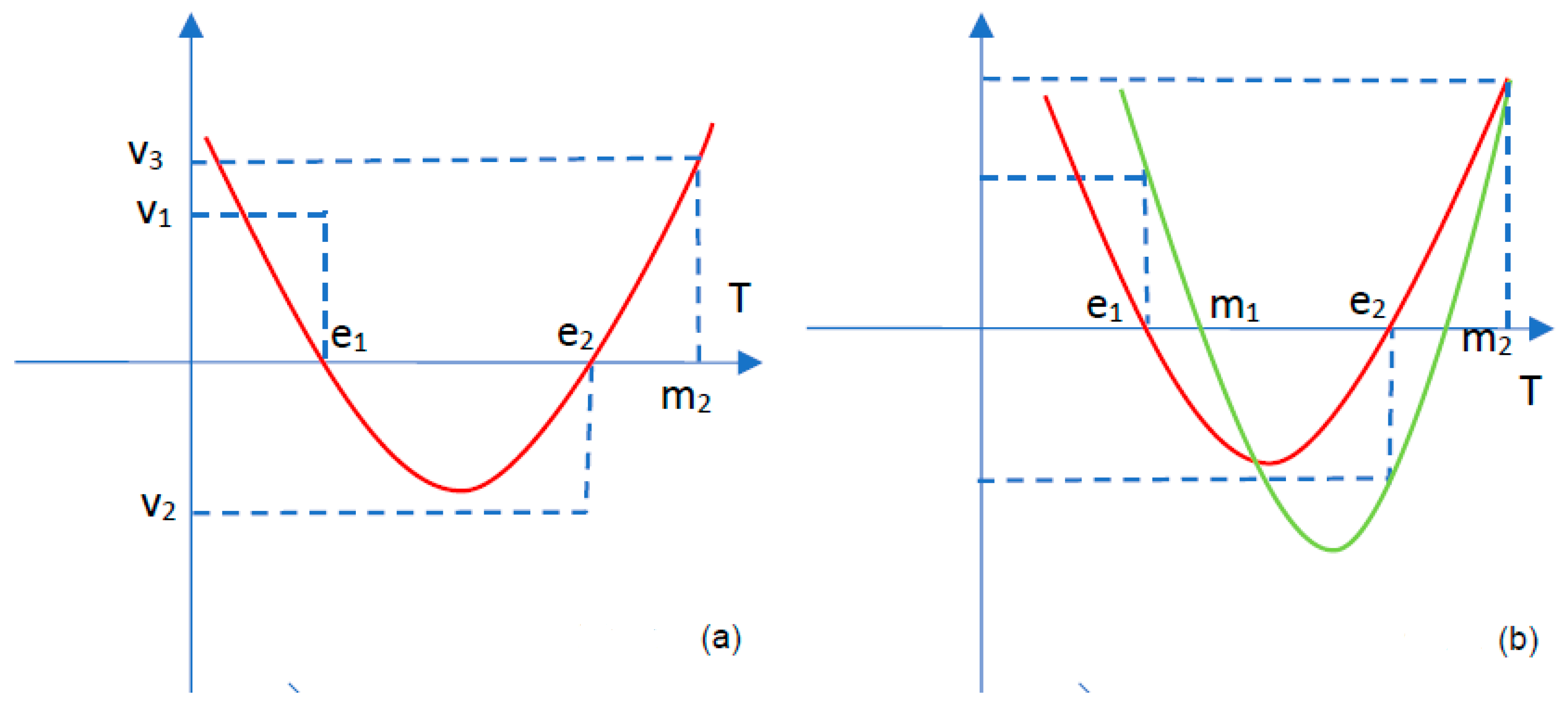
The generic phase portraits corresponding to different regions of the bifurcation diagrams, for different regions are given in
Figure 1 from [
1]. That includes the phase portraits for the curves of bifurcation given by
The smooth functions
can be written as
and
, and the transformation (
8) is not regular at
This means that the Chenciner bifurcation
degenerates, if and only if
Remark 1. In [1], the case when (12) is satisfied with non-zero terms, has been studied—that is, Furthermore, it was assumed before that the linear part of nullifies while has at least one linear term. Thus, the degeneracy condition (12) remains valid while the functions become and
for some
and
where
This can be denoted by
and
respectively,
and
Denote also by
and
C the sets of points in
and
for some
that is sufficiently small. The expression
becomes
where
and
Assume
When
and
this condition is satisfied in general since
Notice that
We can mentioned the following result which is proved by a similar argument as in [
1], Theorem 1:
Theorem 2. (1) The set is a smooth curve of the form tangent to the line (2) If the set is a reunion of two smooth curves of the formwhere and If then for (3) If the set C is a reunion of two smooth curves of the formwhere and If then for Remark 2. In this work, it will assumed instead that and
3. Results
Analysis of degenerate Chenciner bifurcation when will be presented below, in this section.
When the linear part of
and
from (
13) and (
14) is nullified, we can obtain
Then
where
In the truncated case we denoted that
3.1. The Case
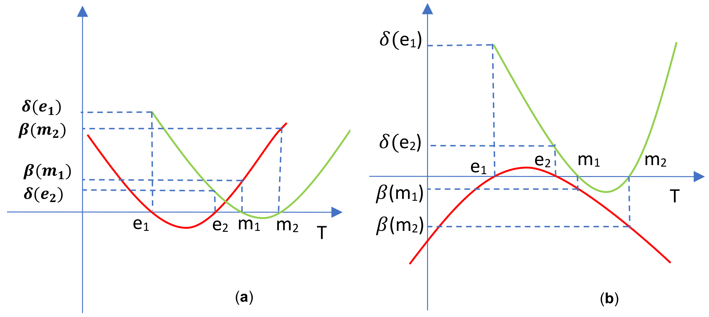
Associated with any of the three above 2-variables polynomials is a 1-variable polynomial, for example,
The order among the roots of , of may be only one of the following ones:
I: II: III:
IV: V: VI:
The roots
are the slops of the straight lines of equations:
of the plane
They are the vanishing loci of the polynomials
We are interested in the configuration of the lines
It is sufficient to consider only cases I and II, since the others are rotated configurations of those. The bifurcation diagram does not depend on the rotation of configurations.
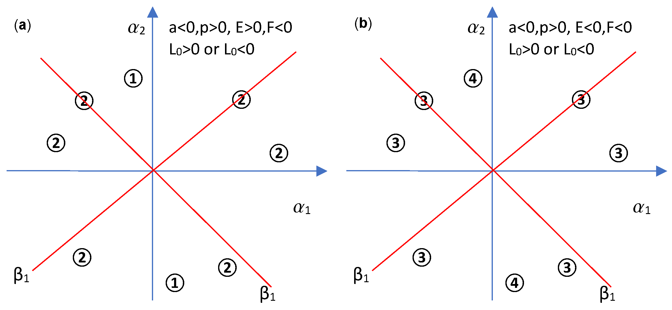
Case I a: see
Figure 1a.
Case I b: see
Figure 1b.
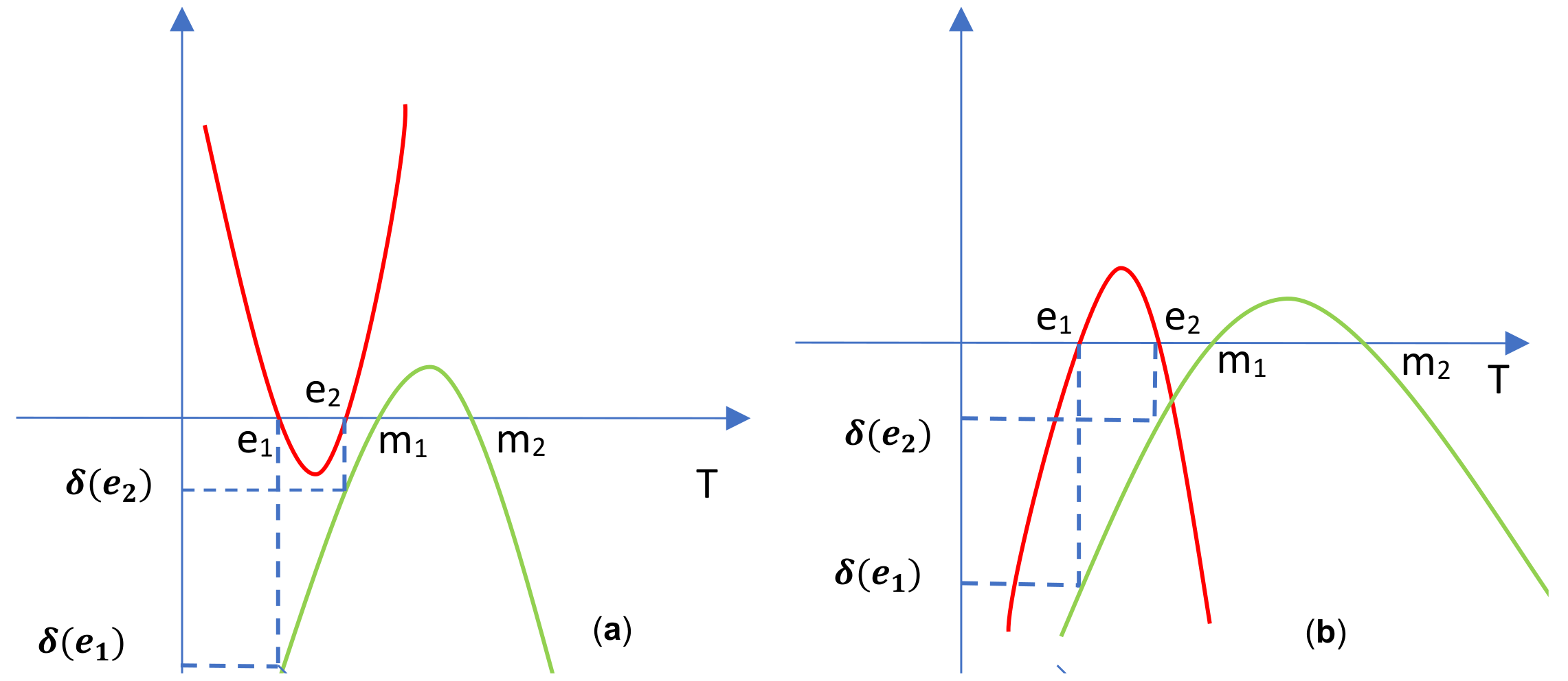
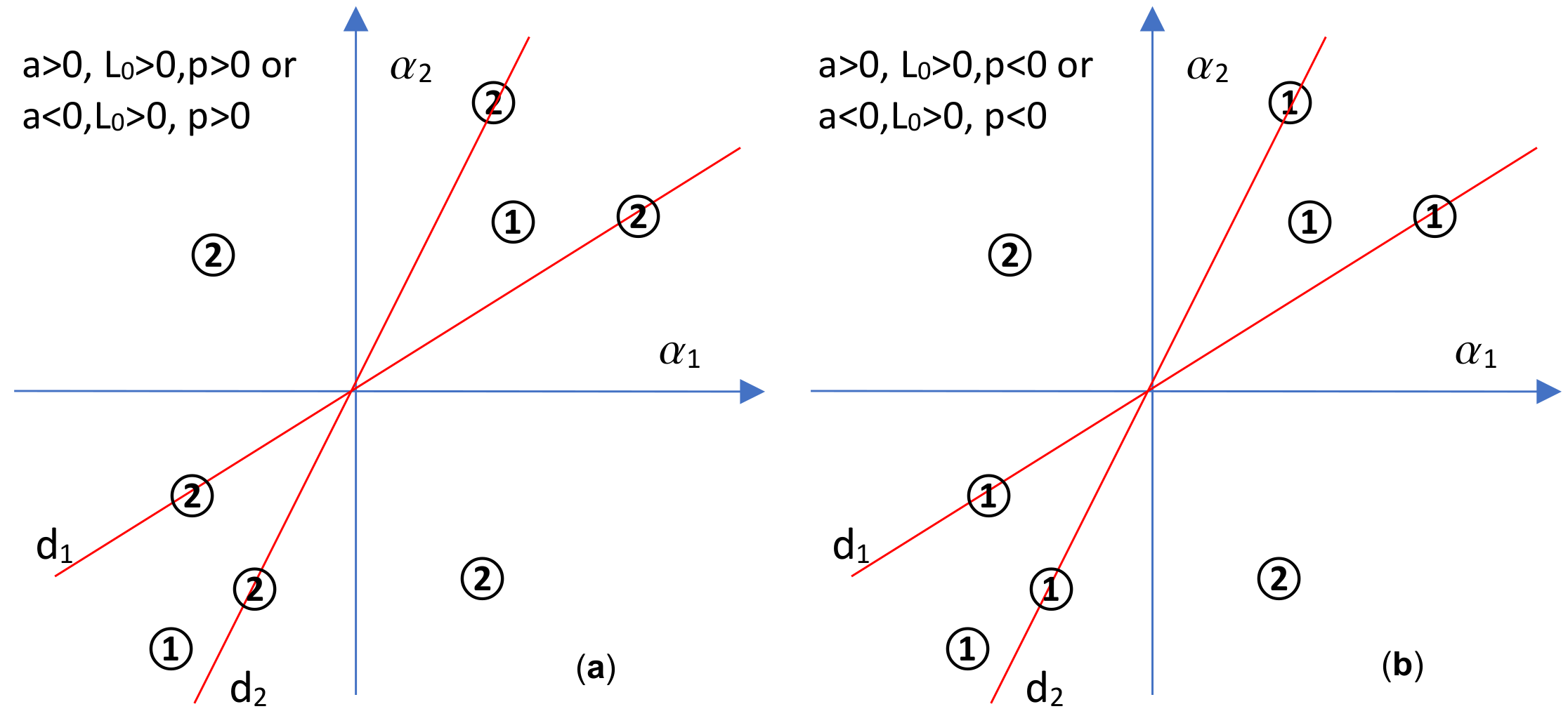
Case I c: see
Figure 2a.
Case I d: see
Figure 2b.
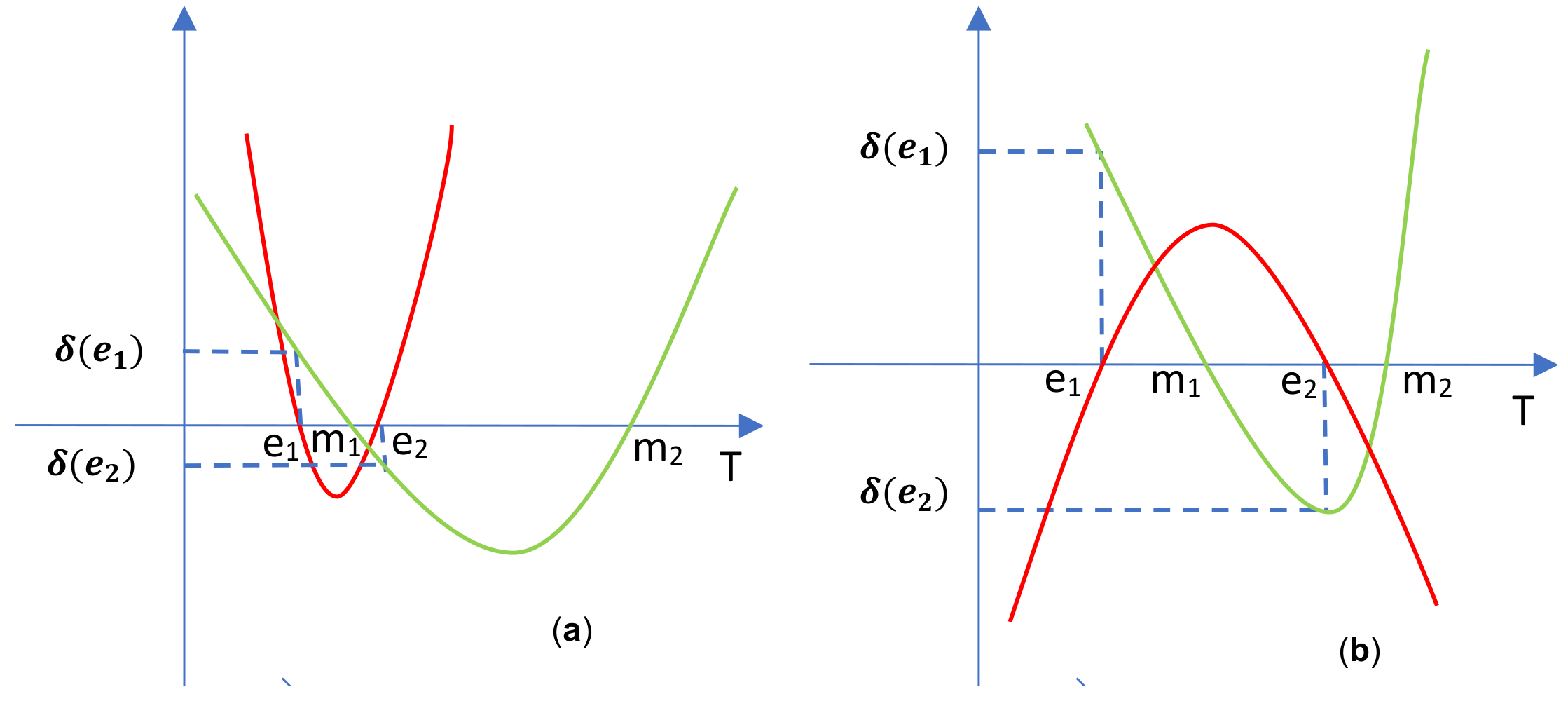
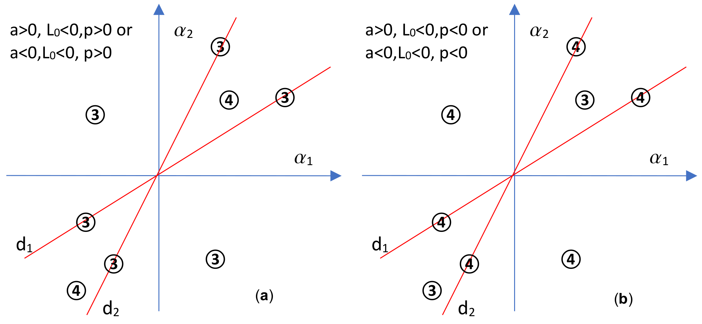
Case II a: see
Figure 3a.
Case II b: see
Figure 3b.
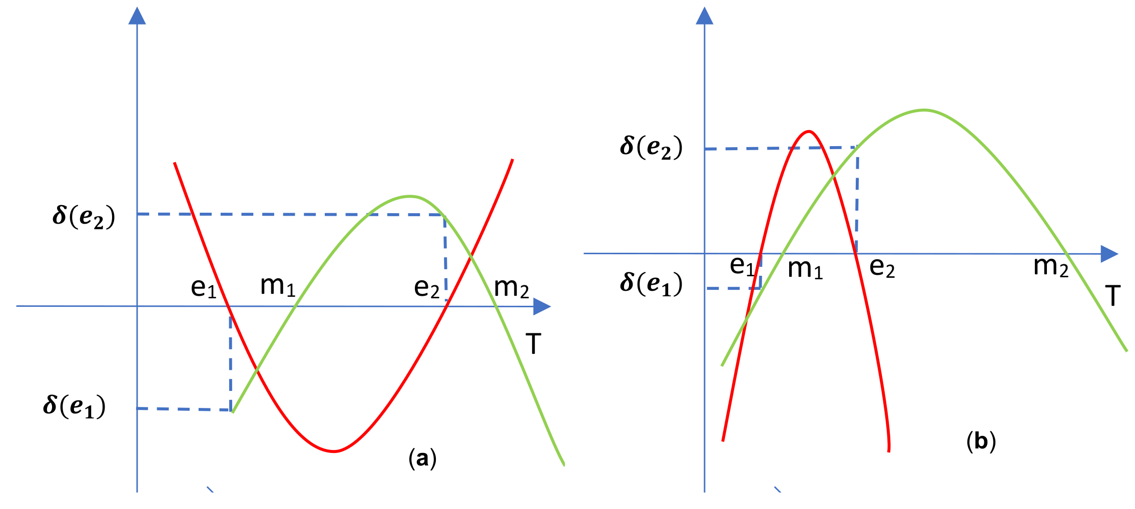
Case II c: see
Figure 4a.
Case II d: see
Figure 4b.
Proof. (1) and by the Viete relation for we get the result.
(2) For the second equality it is sufficient to use the symmetry in the triplets and □
For the sake of simplicity, we will used the notation:
Theorem 3. In case I, if then
Proof. In
Figure 1a,b and
Figure 2a,b, one may take the particular case when the two parabolas have the same symmetry axis, and that does not influence the bifurcation diagrams. That is
hence
The supposition
is equivalent to
, and that it is equivalent to
Let us suppose that
; then, (
24) is equivalent to
and by (
23) that is
and that is
If
then (
24) is equivalent to
or to
or to which eventually is equivalent to □
Corollary 1. By examining Figure 1a,b and Figure 2a,b, it can be concluded that subcases I b,c fulfill the property of Theorem 3, whereas subcases I a,d fail. Therefore I a,d are eliminated. Lemma 2. In case II, there are examples of second degree polynomials such that E and F may have any combination of signs.
Proof. Let us consider a polynomial
having
, and the given numbers
The sum
may be positive or negative(the reasoning will be the same); see
Figure 5a a for
Let us consider a third positive number Then there is such that Now we will consider the parabola determined by the points
,
,
see
Figure 5b.
That is the graph of The sum depending on , may take any value of the interval where Thus, F, which is
may be positive, or negative, and that does not depend on the sign of E, which is □
Theorem 4. In case II:
(1) If and , then
(2) If and , then
(3) If and , then
(4) If and , then
Proof. In all subcases 1–4:
hence,
(1) If
then by (
25):
Considering
, that is equivalent to (
24), which is equivalent to:
By multiplying (
25) by (
26), one gets:
and hence
or
and that is
(2) If
then out of (
25) one gets
is equivalent to (
24) or to
On the other hand, by multiplying (
25) by (
27), is obtained:
and by transitivity
or
which is
.
(3) If
then (
27) is true again, and for
it results in
or
Multiplying (
25) by (
27):
therefore,
or
which is
.
(4) If
then (
26) is true; and if
, then (
28) is also true. The results show that (
24) is true and multiplying (
25) by (
26) will be the result,
and by transitivity
or
which is
□
Corollary 2. Out of Theorem 4 and Lemma 2, one should deduce that case II is not possible; hence, it is eliminated.
In deducing the bifurcation diagrams, one should notice that
implies
out of (
22). The bifurcation diagrams are given in
Figure 6a,b.
3.2. Case 2. and
Therefore we obtained the following four bifurcation diagrams:
(1) For
or
and
(2) For
or
we have
Figure 7a,b:
(3) For
or
and
(4) For
or
will result
Figure 8a,b:
3.3. Case 3.
,
and
The bifurcation diagrams has a single region, which may be:
(1) Region 2 for and
(2) Region 3 for and
(3) Region 1 for and
(4) Region 4 for and
3.4. Case 4.
The rule of signs is simple: and
Moreover,
The bifurcation diagram has also a single region which may be:
(1) Region 2 for and
(2) Region 3 for and
(3) Region 1 for and
(4) Region 4 for and
The results obtained could be applied in cases of phenomena and processes (from different fields of activity—from economics, to biology or medicine and so on) for assimilation into discrete systems in which degenerate Chenciner bifurcations would be identified.
An illustrative numerical example can be presented as an application of the obtained results;
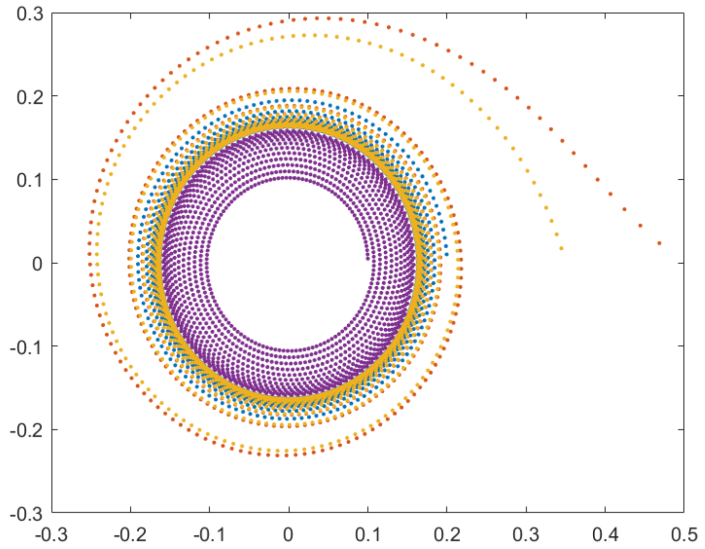
In the following we provide some numerical simulations run using MATLAB. Considering
,
and
and taking as starting points first
, then
and then
. Three orbits will be obtained (
Figure 9). If the starting point is considered now
, then the fourth orbit will appears inside of previous three orbits. The fourth orbit (magenta) departs from the origin and approximates an invariant circle. The previous three orbits approximate the same invariant closed curve, a circle like that of orbit four, when n increases to infinity. In this case the closed invariant circle is stable (
Figure 9). Here
so it is Case 3.3 (2), so the bifurcation diagram has a single region, region 3.


