Attention Optimized Deep Generative Adversarial Network for Removing Uneven Dense Haze

Abstract

The existing dehazing algorithms are problematic because of dense haze being unevenly distributed on the images, and the deep convolutional dehazing network relying too greatly on large-scale datasets. To solve these problems, this paper proposes a generative adversarial network based on the deep symmetric Encoder-Decoder architecture for removing dense haze. To restore the clear image, a four-layer down-sampling encoder is constructed to extract the semantic information lost due to the dense haze. At the same time, in the symmetric decoder module, an attention mechanism is introduced to adaptively assign weights to different pixels and channels, so as to deal with the uneven distribution of haze. Finally, the framework of the generative adversarial network is generated so that the model achieves a better training effect on small-scale datasets. The experimental results showed that the proposed dehazing network can not only effectively remove the unevenly distributed dense haze in the real scene image, but also achieve great performance in real-scene datasets with less training samples, and the evaluation indexes are better than other widely used contrast algorithms.

1. Introduction

Images collected by the imaging sensor are seriously affected by the atmospheric environment such as haze, and therefore lose a lot of contextual information. The purpose of image dehazing is to eliminate the negative impact of the atmospheric environment on image quality and increase the visibility of the image (Figure 1). It also provides support for downstream visual tasks such as image segmentation.

Image dehazing is mainly divided into traditional algorithms and learning-based algorithms. The traditional dehazing algorithms use the atmospheric scattering model [1,2,3,4] to simulate the generation of haze. Usually, they need additional prior knowledge to detect the distribution of haze. When haze is located, the parameters of the atmospheric scattering model can be used to solve the dehazed image. The atmospheric scattering model can be formulated as [1,2]:

$$I\left(z\right)=J\left(z\right)t\left(z\right)+A\left(1-t\left(z\right)\right),$$

(1)

where I(z) is the observed hazy image, and J(z) is the corresponding haze-free image. A is global atmosphere light, and t(z) is the medium transmission map. Moreover, the transmission map is formulated as [1,2]:

$$t\left(z\right)=e^{-\beta d\left(z\right)},$$

(2)

where β is the atmosphere scattering parameters, and d(z) is scene depth. As can be seen from the above two formulas, once global atmosphere light, atmosphere scattering parameters, and scene depth can be correctly calculated, we can directly restore the haze-free image from a hazy input.

Based on the atmospheric scattering model, a lot of early traditional dehazing algorithms [5,6,7,8,9,10,11,12,13,14,15] are proposed. Among them, dark channel prior (DCP) [5] is the most successful traditional dehazing algorithm. Through the statistics of many real haze-free images, it is found that most local color blocks of haze-free images contain some pixels with very low intensity in at least one color-channel. Through this prior knowledge, DCP method can quickly locate the hazy area in an image and solve the global atmosphere light and coarse transmission map. However, because DCP method is sensitive to pixel intensity, it usually fails in high brightness areas such as the sky, which limits its practical application. Other traditional dehazing algorithms are also facing the problem of large errors when estimating parameters and are therefore difficult to apply to sophisticated real scenes.

With deep learning making great strides in the field of image processing [16,17,18,19,20], the convolutional neural network (CNN) also shows good application prospects in the field of single image dehazing. Many learning-based algorithms [21,22,23,24] have been proposed and achieved better performance over traditional algorithms. Some learning-based dehazing algorithms learn the transmission map, atmosphere light, scene depth and other key parameters through large-scale datasets, so as to calculate the predicted dehazing image according to the atmospheric scattering model. Inspired by other low-level image task algorithms, the latest dehazing model selects a direct end-to-end network to avoid employing the atmospheric scattering model [25,26,27,28]. This design can not only avoid the error accumulation caused by the atmospheric scattering model, but also be more conducive to the support of downstream high-level semantic tasks.

Although the learning-based image dehazing algorithm has achieved good results, it still faces the following problems. First, the performance of the complete end-to-end network depends heavily on the training results on large-scale datasets. Most of the dehazing datasets are synthesized by computer simulation [29,30], which is far from the real scene, and the large-scale real scene dehazing datasets are difficult to obtain, which limits the performance of the model. Second, most of the existing methods deal with the pixels on the image equally, which cannot deal with the uneven haze in the real scene.

As a result of the two problems mentioned above, this paper proposes an attention optimized deep symmetrical encoder-decoder generative adversarial network for removing uneven dense haze in real scene. This network is fully end-to-end. When inputting a hazy image, it can directly generate the corresponding haze-free image without calculating other parameters. We use the generative adversarial network (GAN) [31] as the main structure of the method, which makes our model robust on small-scale datasets. The densely connected four-layer down-sampling structure is used to fully extract the deep semantic information lost by dense haze. At the same time, local residual learning block is utilized to ensure that the shallow information such as outline, contrast and texture will not disappear when transmitted to the deep layer. After the information is encoded, a symmetrical four-layer upsampling decoder is employed to restore the features to the original resolution. Because the haze is usually unevenly distributed in the real scene, it is unreasonable to directly give the same weight to the multi-channel and each pixel of the feature map. Therefore, we apply the attention mechanism [32] to the decoder network to learn the distribution of haze in spatial domain and channel domain. Through these designs, our method can more effectively eliminate the haze in the image and output a more real haze-free image. Experiments show the network performs much better than the widely used dehazing algorithms.

Our contributions are as follows:

• We propose a fully end-to-end network for single image dehazing. It can output a haze-free image directly from one hazy image without calculating intermediate parameters. Our method uses a generative adversarial network as the framework, which makes our network more robust, and even trained in a small-scale dataset.
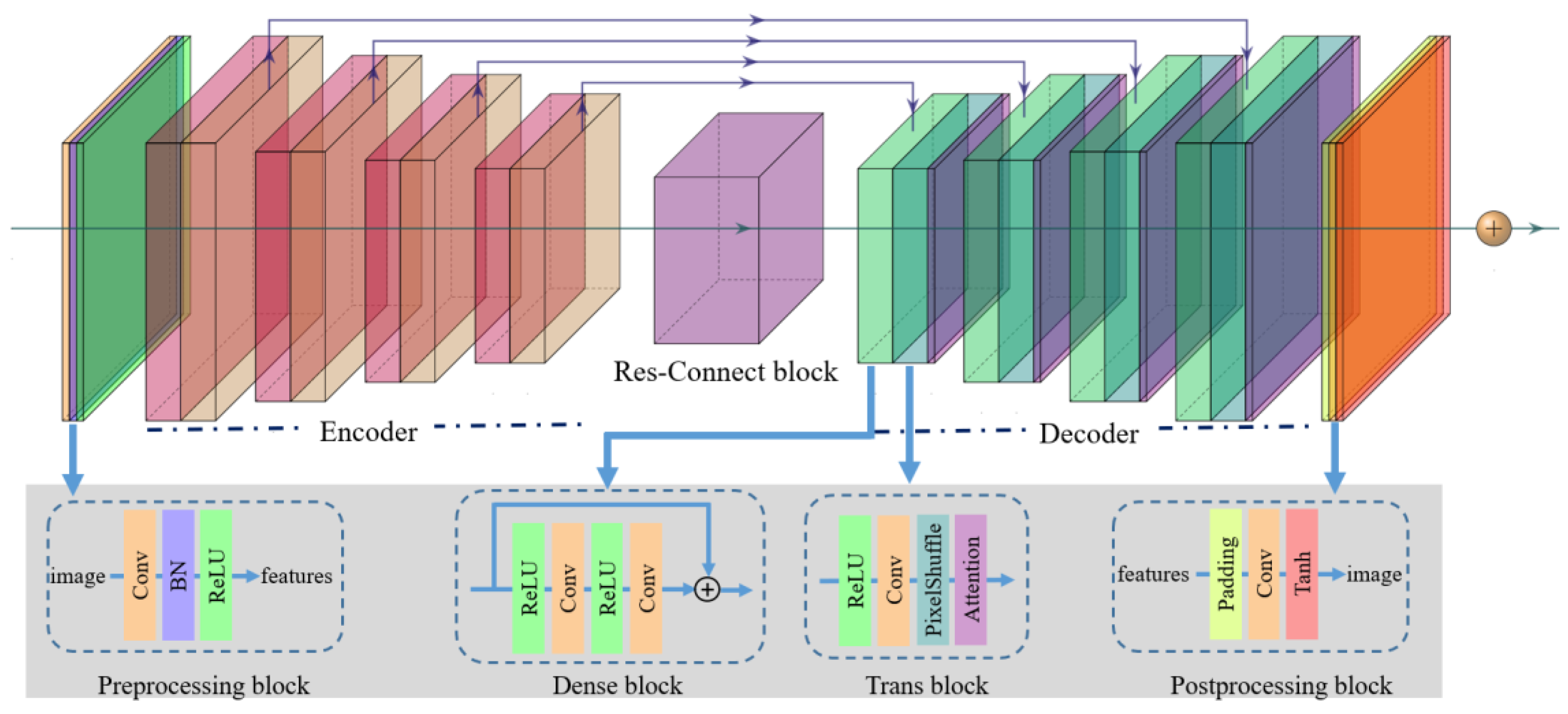
• To better extract the semantic information degraded due to the dense haze, we employ a densely connected four-layer down-sampling. At the same time, the local learning mechanism is also introduced to allow the information of the thin haze region and low-frequency information to be passed through the down-sampling operation and be reserved.
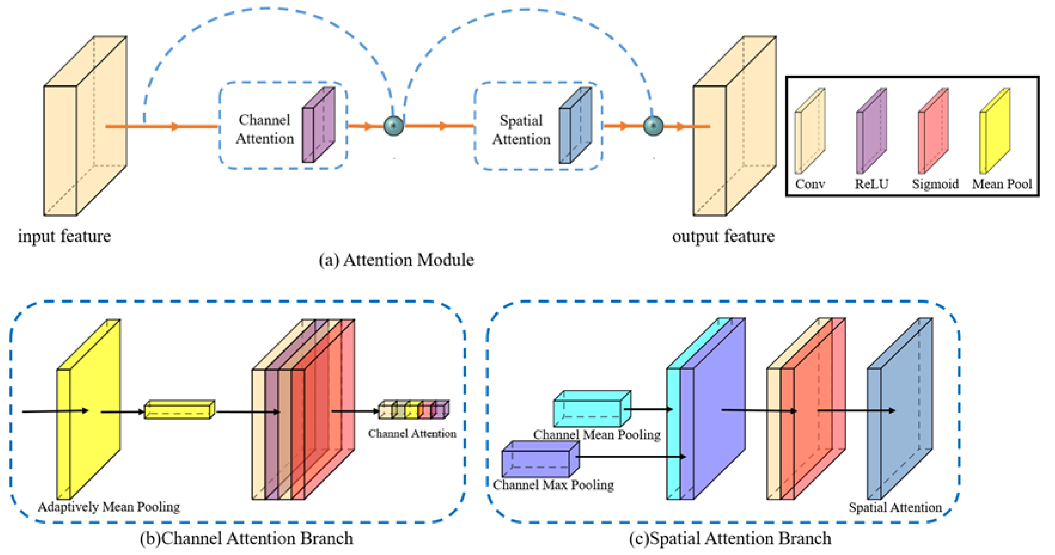
• Spatial attention and channel attention module are introduced to our method. Considering the uneven distribution of haze in space and different feature channels have different sensitivity to haze concentration, it is not appropriate to use the same weights for them. Attention module allows for the assignment of different weights to different locations and channels, which helps the network to learn the uneven distribution haze and better deal with uneven dense haze.

2. Related Works

2.1. Traditional Algorithms

DCP [5] method is the most classical dehazing algorithm based on statistical prior knowledge. However, it usually fails when the background light intensity is high. To solve the shortcomings of DCP method, He et al. further propose the guided filter dehazing algorithm [8]. Because the haze noise is usually characterized by large gradient and little difference in all directions centered on it, guided filter dehazing algorithm locates the haze area independent of the background light. However, this method is usually accompanied by color distortion that cannot be ignored. Zhu et al. propose a color-attenuation-prior-based dehazing algorithm [6]. They create a linear model to calculate the scene depth of the hazy image. Fattal finds a generic regularity in natural images known as color-lines [9] to recover the scene transmission based on the lines’ offset from the origin. Although a considerable amount of prior knowledge [7,10,11,12] has been applied to traditional dehazing algorithms to improve their performance, these algorithms still face the problem of insufficient robustness. When the prior knowledge is not satisfied, the effect of these algorithms will be seriously affected.

2.2. Learning-Based Algorithms

With deep learning making great strides in the field of image processing, learning the difference between hazy and haze-free images with the help of the powerful learning ability of the neural network, and then restoring haze-free images, has become the mainstream dehazing algorithm. The early learning-based dehazing algorithms still use the atmospheric scattering model. They used the fitting ability of the neural network to estimate parameters such as scene depth and transmission map. DehazeNet [21] is one of the first end-to-end dehazing networks based on a deep learning architecture. It learns the transmission rate map in the atmospheric scattering model from hazy images and recovers haze-free images accordingly. The design of each layer of the network reflects the idea of prior knowledge such as DCP. Zhang et al. propose a densely connected pyramid network called DCPDN [22] to jointly learn the transmission map, atmosphere light and dehazing all together. Its network structure is two parallel subnetworks; a pyramid densely connected module for calculating the transmission map and a U-net-based [33] subnetwork for estimating atmosphere light. Ren et al. propose a multi-scale deep neural network called MSCNN [23]. Given a hazy input, the network can recover a potentially haze-free image by estimating the scene transmission map. This network consists of a coarse-scale subnetwork for predicting a holistic transmission map and a fine-scale subnetwork for refining results locally. AOD-Net [24] is an end-to-end dehazing network based on an improved atmospheric scattering model, which does not require any additional parameters to be computed during training. AOD-Net can be seamlessly integrated with subsequent high-level vision tasks. However, there will be errors in predicting the parameters of the atmospheric scattering model. Moreover, the atmospheric scattering model itself is a simulation of the causes of haze formation. Therefore, even the dehazed images generated by the learning-based dehazing algorithm are still quite different from the real haze-free images.

In order to avoid the error caused by atmospheric scattering model, the latest dehazing algorithms adopt a fully end-to-end structure [25,26,27,28], which means that the haze-free image is generated directly from the hazy image and the calculation of intermediate parameters is ignored. Ren et al. propose a gated fusion dehazing network for single image dehazing [25]. The constructed network adopts three image pre-processing methods for image enhancement. The network will learn the confidence feature map to process the three pre-processed images obtained from the original image to automatically obtain the proportion of these three image features in the final output image. At last, the final dehazed image is yielded by gating the important features of the derived inputs. Inspired by visual perception global-first theory, Qu et al. design an enhanced pix2pix dehazing network (EPDN) [26] embedded by a generative adversarial network (GAN). EPDN consist of a discriminator for guiding the generator to create more realistic images and a generator followed by a receptive-field-model-based enhancer used to reinforce the dehazing effect in both color and details.

2.3. Generative Adversarial Network

The GAN [31] model was first proposed by Goodfellow et al. to synthesize realistic images by effectively learning the distribution of the training images. GAN usually consists of a discriminator network and a generator network. The discriminator network is used to judge whether the sample generated by the generator network is true or false. After receiving the feedback, the generator network will generate more real samples to deceive the discriminator network. In such a game process, the whole GAN network will have a more powerful performance. GAN structure has been introduced in some low-level image restoration tasks [34,35,36,37,38,39]. Similarly, the dehazing algorithm based on GAN also began to appear [40,41,42,43].

3. Methods

3.1. Overall Framework

Our network adopts the architecture of generative adversarial network, which is divided into generator network and discriminator network. The generator network receives the input hazy image and generates the dehazed image. The discriminator network receives the dehazed image generated by the generator and the corresponding ground truth image. It will identify whether the images generated by the generator network are true or false and supervise the generator network to continue training according to the corresponding results. In this model, as shown in Figure 2, the generator network adopts a densely connected four-layer down-sampling encoder structure to fully extract the text information of the image. At the same time, the skip-connection strategy is also applied to ensure that the shallow information is not lost in the transmission process and prevent the gradient from disappearing. The decoder module adds a specially designed attention module to deal with the unevenly distributed haze. As shown in Figure 3, the discriminator network is a common binary classification network. By generating the framework of generative adversarial network, the model can reduce the requirements for large-scale training datasets and broaden the application scenario of the model.

3.2. Four-Layer Down-Sampling Encoder with Dense Residual Connection

Fewer convolution layers can only extract shallow features, while more convolution layers can extract deep features. Shallow information is usually syntax information, such as outline, color, texture and so on [40]. Deep information is usually semantic information that is difficult to perceive. Due to the existence of dense haze, the shallow features of the input image become imperceptible, which is reflected in color distortion and edge virtualization. Compared with other networks, DenseNet is better at exploring the inlining between features and extracting deeper features. Inspired by the method of using multi-layer down-sampling operation as encoder, we design a densely connected four-layer down-sampling encoder to fully extract the contextual information covered by dense haze. The encoder uses DenseNet-121 [44] pre-trained on ImageNet [45] dataset as feature extractor. DenseNet’s remarkable feature is the use of densely connected residual network. Compared with simply stacking convolution layers directly or extracting features using Resnet [46], DenseNet not only fully extracts image contextual information, but also improves feature utilization without introducing additional parameters, which is conducive to recovering image information lost due to high concentration haze. In addition, it establishes sufficient skip-connections between different layers. Through the structure of skip-connections, the features extracted from the previous layer are integrated into the current layer to ensure the accuracy of visual tasks. The encoder structure is shown in Figure 2. Firstly, we introduce a preprocessing process, which includes a convolutional (Conv) layer, a batch-norm (BN) layer and a rectified linear unit (ReLU) layer. The original features obtained after preprocessing are then sent to the encoder. The encoder includes four groups of pre-trained denseblock and transblock. Both denseblock and transblock layers are standard DenseNet-121 block. After pre-training on the ImageNet dataset, the pre-training weights are used to replace the random initialization weights, which can speed up the convergence of the model. The transblock of each layer contains a max-pool layer, which will reduce the features by half, and four-layer down-sampling finally reduces the feature map to one sixteenth of the original size.

3.3. Attention Optimized Decoder

Because the encoder reduces the feature size to one sixteenth of the original size, a symmetrical four-layer upsampling module is required to recover the feature size. Similar to the encoder, we use four symmetrical groups of denseblock and transblock. This symmetrical codec module design can make it easier for shallow features to be integrated into deep features through skip-connection. However, the denseblock and transblock of the decoder are different from those in the encoder, which are specially designed and simplified. The purpose is to process the sampled feature map and restore the size of the feature map to the size of the original picture. The simplified structure of denseblock and transblock is shown in Figure 2. The denseblock of each decoder includes two groups of ReLU layers and Conv layers. In order to restore the size of the feature map to the original size, each transblock must contain an upsampling operator. Compared with direct quadratic linear interpolation for upsampling, this paper uses the learnable upsampling module called pixelshuffle (as shown in Figure 4) [47] to avoid artificial traces caused by interpolation during upsampling. It is more suitable for end-to-end image tasks.

Usual dehazing method assigns uniform weights to all pixels and channels, which is inconsistent with the real experience. Because the haze is unevenly distributed in the real scene, setting the same weights for all pixel values will lead to insufficient dehazing in areas with higher haze concentration and affect the final image restoration quality. Moreover, for all channels of the feature map, their sensitivity to haze concentration is also different. Therefore, in the reconstruction of the feature map, the introduction of the attention module helps the network better learn the haze distribution and achieve a more ideal dehazing effect. Different from other dehazing methods using the attention mechanism [48,49,50], after each transblock in decoder, we add an attention module, whose structure is shown in Figure 5. Inspired by literature [32], the attention module is divided into channel domain attention branch and spatial domain attention branch. In channel domain attention branch, we first take the average value of all pixels of each channel of the feature map in the decoder as the original channel attention feature vector. For a c*h*w feature map, we can produce a feature vector of c*1 size. The channel attention of k-th channel can be formulated as [32]:

$${\mathsf{A}}_c^k=\frac{1}{h\ast w}{{\displaystyle \sum }}_{i=1}^h{{\displaystyle \sum }}_{j=1}^{w}valu{e}_k\left(i, j\right),$$

(3)

where $valu{e}_k\left(i, j\right)$ means the pixel value of $k$-th channel at position $\left(i, j\right)$.

In order to enable the feature vector to learn the sensitivity of different channels, we perform Conv, ReLU, Conv and Sigmoid operations on it in turn. In this way, the feature vector can learn the attention of different channels through training. Finally, we multiply the attention vector with the original feature map.

The calculation of attention in spatial domain is similar to that in channel domain. For the obtained channel attention feature map, we first perform average pooling and maximum pooling along the channel dimension to obtain two $1\ast h\ast w$ original spatial attention. The pixels at each point on the feature map are the average and maximum values of all pixels at that position on all channels. Average spatial attention at position $\left(i, j\right)$ can be formulated as [32]:

$$A_{s, avg }^{\left(i, j\right)}=\frac{1}{m}{{\displaystyle \sum }}_{k=1}^{m}valu{e}_k\left(i, j\right),$$

(4)

where $m$ is the number of feature channel.

Then, Conv and Sigmoid operations are performed on the two feature maps to obtain the learned spatial domain attention. Finally, the spatial domain attention is multiplied by the feature map mixed with channel domain attention. The uneven distribution of haze in channel and space is learned by feature map.

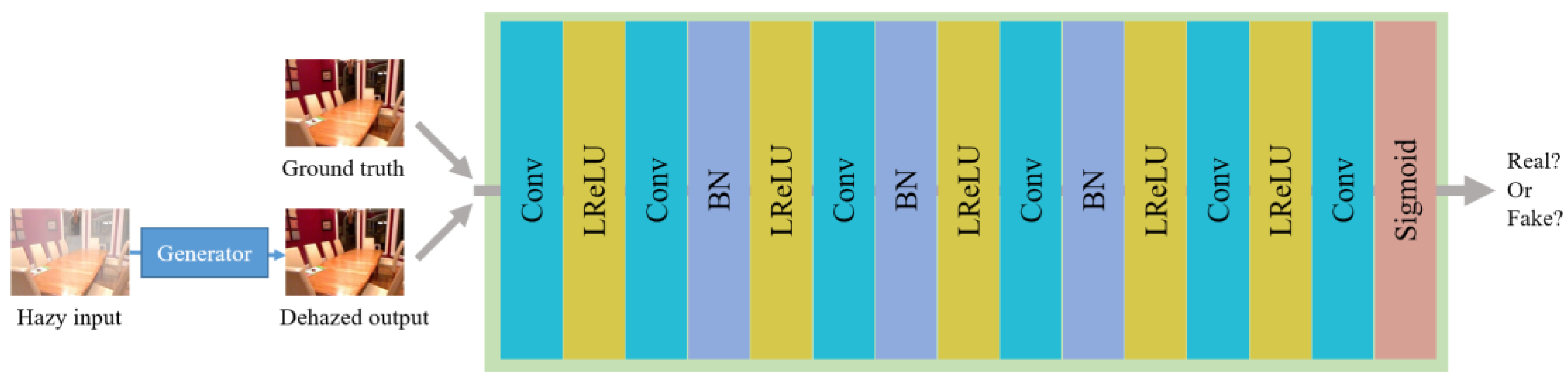
3.4. Discriminator Network

The discriminator network is a conventional binary classification network. Its input is a symmetrical image pair consisting of the dehazed image generated by the generator and the corresponding haze-free image. The output of the discriminator network is to identify whether the image is true or false and guide the generator network training accordingly. In the training process, the discriminator will improve the ability to identify true data and false data as much as possible, and the generator will generate true data as much as possible. The discriminator uses real data and false data for training to update the weight. When the generator is trained, it will use the complete model with frozen discriminator. At this time, the false data generated by the generator is output to the discriminator and the false data is marked as true data. The parameter update of the generator network is realized by transmitting the error of the discriminator forward, which means that the weight update of the generator is guided by the discriminator. In the discriminator, we use a series of combinations of LeakyReLU [51] layer, Conv layer and BN layer. In the process of gradient back propagation, LeakyReLU function (as shown in Figure 6) adds an extra hyperparameter to calculate the gradient when the input of the activation function is less than 0, which solves the problem of neuron death due to the emergence of negative samples. The BatchNorm layer can centralize and standardize each batch. This operation can avoid the continuous increase in parameters when the parameters change too much due to a different data distribution. Of course, it can also avoid gradient explosion and accelerate the convergence speed while using a more accurate learning rate. These two layers have good applications in classification networks.

3.5. Loss Function

In order to comprehensively consider all aspects of the performance of the generated haze-free image and better guide the model to complete the training, we use an integrated loss function consisting of reconstruction loss, perceptual loss [52], and adversarial loss.

The reconstruction loss measures the average absolute error between the output dehazed image and the corresponding reference image, and can be formulated as:

$$L_r=\frac{1}{n}{{\displaystyle \sum }}_{i}L1(G\left(I_i\right)-J_i),$$

(5)

where $I$ means the hazy input of the generator, and $J$ stands for the corresponding ground truth haze-free image. $G(·)$ means the generator, and $L1(·)$ represents least absolute error. Reconstruction loss can measure the distortion on pixel value between dehazed image and ground truth but is often inconsistent with human visual perception. Therefore, perceptual loss is proposed to solve this problem.

Perceptual loss is formulated as [52]:

$$L_p=\frac{1}{n}{{\displaystyle \sum }}_{i}L2\left(vgg\left(G\left(I_i\right)\right)-vgg\left(J_i\right)\right),$$

(6)

where $L2(·)$ means least square error, and $vgg(·)$ means pre-trained VGG16 network [53]. VGG16 network is also a network trained in ImageNet. It can extract image edge, color, brightness, texture and even deeper imperceptible semantic features. Simulating the difference of human eye perception of the image with VGG16 is also widely used in tasks such as super-resolution and style migration.

Finally, the adversarial loss is also integrated into the loss function to reflect the guiding role of the discriminator network to the generator network. It is formulated as [31]:

$$L_a=\frac{1}{n}{{\displaystyle \sum }}_i\left(-\log {\displaystyle (}1-D{\displaystyle (}G\left(I_i\right){\displaystyle )}{\displaystyle )}\right),$$

(7)

where $D(·)$ means the discriminator.

Finally, we combine the reconstruction loss, perceptual loss and adversarial loss together to regularize our network.

$$L=\alpha L_r+\beta L_p+\gamma L_a,$$

(8)

In our experiment, $\alpha$, $\beta$, $\gamma$ are set to be 1, 0.9, 0.1 correspondingly.

4. Experiments

4.1. Datasets and Metrics

Considering the application effect in real scene, we selected small-scale real-world datasets I-HAZY [54] and O-HAZY [55]. The I-HAZY and O-HAZY datasets are proposed to solve the problem that the current learning-based dehazing method relies too much on large-scale synthetic datasets. Compared with the most commonly used dehazing datasets, I-HAZY and O-HAZY datasets are more challenging for the performance of the model. The I-HAZY dataset includes 30 pairs of indoor real hazy images and corresponding haze-free images, of which 25 pairs are used for training and five pairs are used for testing. The O-HAZY dataset includes 45 pairs of outdoor real hazy images and corresponding haze-free images, of which 40 pairs are used for training and five pairs are used for testing. The real hazy images are generated by a professional haze generator. They are taken under the same illumination parameters as the corresponding haze-free images, which is closer to the practical application.

In this paper, two objective performance indexes and one subjective index commonly used in image restoration are used to evaluate the performance of the model proposed in this paper, and compared with other dehazing methods. The objective indexes are peak signal to noise ratio (PSNR) and structural similarity index (SSIM) [56]. The subjective index is Learned Perceptual Image Patch Similarity (LPIPS) [57].

PSNR is used to measure the pixel-wise error between the image and the corresponding reference image. PSNR is an error sensitive image quality evaluation index, and is formulated as:

$$PSNR=10lo{g}_{10}\left(\frac{{\left(2^n-1\right)}^2}{MSE}\right),$$

(9)

where $n$ represents the bit width of the pixel, and $MSE$ stands for the mean absolute error.

SSIM considers the error between the dehazed image and the corresponding reference image from three aspects: brightness, contrast and structure. Compared with PSNR, SSIM is more comprehensive and according with people’s intuitive feelings. SSIM is formulated as:

$$\{\begin{array}{l}l\left(x, y\right)=\frac{2{\mu }_x{\mu }_y+c_1}{{\mu }_x^2+{\mu }_y^2+c_1}\\ c\left(x, y\right)=\frac{2{\sigma }_x{\sigma }_y+c_2}{{\sigma }_x^2+{\sigma }_y^2+c_2}\\ s\left(x,y\right)=\frac{{\sigma }_{xy}+c_3}{{\sigma }_x{\sigma }_y+c_3}\end{array},$$

(10)

$$SSIM=l\left(x,y\right)\ast c\left(x,y\right)\ast s\left(x,y\right),$$

(11)

where $\mu$ means mean, ${\sigma }_x$ means variance, and means covariance. $l$, $c$, $s$ stand for brightness, contrast and structure. $c_1$, $c_2$, $c_3$ are constant.

LPIPS uses the similarity measurement of high-dimension image structure to replace the distance measurement that cannot be formed in practice, which means the difference of pixel values is not always consistent with people’s subjective perception. In practical use, LPIPS uses the deep network pre-trained on ImageNet dataset to extract the deep features of images and reference images. The lower the LPIPS value, the higher the feature similarity between the generated image and the corresponding reference image, and the more similar the subjective perception.

4.2. Implement Details

The program in this paper is written in Pytorch framework and trained on computer configured with Intel i9-9900k CPU and NVIDIA GeForce RTX 2080ti GPU. Our initial learning rate is set to 0.0001. Adam [58] is used as the learning rate optimization strategy, and StepLR is used to adjust the basic learning rate periodically. The image is cut to a fixed size of $256\times 256$. Every patch transferred to the generator is randomly rotated by 0°, 90°, 180° or 270° to prevent over fitting. In order to further improve the robustness of the generative adversarial network, we set up a sample pool. When the generator receives 50 pairs of hazy images and corresponding haze-free images, the subsequent image pairs will have a 50% probability to be consisted of a hazy image and a random mismatched haze-free image. The purpose of this sample pool is to prevent the discriminator network from stopping training and supervise the training of the generator network in the small-scale dataset. In the training process, num of threads is set to eight, batch size is set to one, and epoch is set to 5000. Learning rate step is set to 1000 and learning rate decay is set to 0.5. The last two parameters mean that for every 1000 epochs trained, the basic learning rate is attenuated to half of the initial learning rate. The code can be available at [59].

4.3. Experiment Results

The model in this paper is compared with DCP [5], CAP [6], DehazeNet [21], DCPDN [22] and AOD-Net [24]. The visual comparison results are shown in Figure 7, and the experimental results of quantitative analysis are shown in

Table 1. Objective metrics PSNR and SSIM comparisons.

		DCP [5]	CAP [6]	DehazeNet [21]	DCPDN [22]	AOD-Net [24]	Ours
I-HAZY	PSNR	14.43	14.62	15.72	16.21	13.98	22.17
	SSIM	0.752	0.767	0.734	0.755	0.732	0.793
O-HAZY	PSNR	16.78	16.01	16.12	15.16	15.03	22.72
	SSIM	0.653	0.681	0.612	0.673	0.539	0.784

and

Table 2. Subjective metric LPIPS comparisons.

	DCP [5]	CAP [6]	DehazeNet [21]	DCPDN [22]	AOD-Net [24]	Ours
I-HAZY	0.333	0.298	0.313	0.274	0.374	0.218
O-HAZY	0.411	0.675	0.405	0.377	0.445	0.269

, respectively.

4.4. Experiment on Large-Scale Dataset

Although it is better to measure the robustness of the proposed method in the real-scene in small-scale real-world datasets, we also conduct quantitative analysis on a large-scale benchmark for making the experiment results more convincing. Considering the number of samples in the dataset, we select RESIDE as the dataset used for training and testing. RESIDE is a large-scale benchmark including five subsets collected from both synthetic and real-world images. In this experiment, we choose ITS subset, consisting of 10,000 haze-free images as ground truth and their corresponding 100,000 synthetic hazy images, and OTS subset, consisting of 8970 haze-free images as ground truth and their corresponding 313,950 synthetic hazy images for training. For quantitatively analyzing the dehaze performance of our network, we test it on SOST subset, which consists of 500 pairs of haze-free and corresponding hazy images not included in ITS and OTS. We compared our method with four different algorithms: DCP, DehazeNet, DCPDN, AOD-Net, and the results are shown in Figure 8 and

Table 3. Metrics comparisons with other methods on SOTS dataset.

Method	PSNR	SSIM	LPIPS
DCP [5]	16.62	0.818	0.293
DehazeNet [21]	21.14	0.847	0.261
DCPDN [22]	19.98	0.857	0.243
AOD-Net [24]	19.06	0.850	0.228
ours	27.12	0.909	0.213

.

As can be seen from the results, the dehazed images generated from our method are best restored to the ground truth images both in metrics and visualization results. DehazeNet has achieved a relatively high PSNR, which is reflected in the outdoor images. In the RESIDE dataset, the haze of outdoor images is uneven, while the haze of indoor images is related to the depth of field and is uneven. So, when it comes to indoor images, DehazeNet performs badly due to lack of sufficient information extracted by its encoder. The color distortion of DCPDN is obvious, which is consistent with its performance in I-HAZE and O-HAZY datasets. For the high brightness area in the third row of the Figure 8 and the sky area in the fourth and fifth rows of Figure 8, there exists visible color distortion. AOD-Net has a better dehazing effect, but from the perspective of visual perception, the color brightness of the pictures generated by AOD-Net is significantly lower than that of the ground truth. Because a more effective encoder is used to extract contextual information, there is almost no obvious differences between the images generated by our method and the ground truth. At the same time, due to the attention mechanism, its performance is not lost when it comes to indoor images. For the thicker haze caused by deeper depth of field, our method can also learn and remove the haze perfectly.

4.5. Experiment on Real-World Images

In order to show the dehazing effect of our method on real hazy images, we compare the visual quality of different methods on real-world images from RTTS, a subset of RESIDE. Due to the lack of corresponding haze-free images, quantitative analysis cannot be carried out. As shown in Figure 9, our method can remove the haze on the image to the greatest extent, and better restore the contour and color information of the object. The comparison methods have some problems of insufficient dehazing and color distortion to varying degrees. The dehazing of DCP method is more average, which is reflected in that it may well remove the haze on the surface (in the first row of Figure 9), but it is weak for deeper haze (in the second row of Figure 9). DCPDN suffers heavily from color distortion that can not be ignored, which can obviously be seen in the second row. The brightness of dehazed images generated by DehazeNet is lower than ours, and there still exists a strong sense of haze in the images generated by AOD-Net. Overall, our proposed method can best restore details and achieve a pleasing visual appearance.

5. Conclusions

In this paper, we propose an attention optimized deep generative adversarial network for removing uneven dense haze in real scene. Through the framework of generative adversarial network, the model can achieve better training effects in small-scale datasets. The generator network adopts the structure of a deep symmetric encoder-decoder structure. The encoder adopts a densely connected four-layer down-sampling structure to ensure the full extraction of image contextual information and recover the information lost due to the dense haze. Then, a symmetric decoder is used to restore the resolution decreased by the encoder. The attention mechanism is introduced into the decoder, which can adaptively give attention weights to different pixels and channels, so as to deal with the uneven distribution of haze in the real scene. The experiment results on I-HAZY and O-HAZY datasets show that compared with the widely used dehazing algorithms and models, our model has excellent performance in both objective metric and subjective visual perception.

Although the proposed network has achieved good results in removing haze in real scenes, it can still be improved in the following aspects. First, the network adopts a relatively simple structure design, namely symmetrical encoder-decoder, so its encoder and decoder can be adjusted quickly. Designing a more effective feature extraction backbone network will help to improve the ability of dehazing. Second, the special loss function design will also help to improve the dehazing metrics of the model, such as SSIM loss function designed in [40]. Finally, the proposed method is also suitable for other low-level visual tasks, such as decloud, derain, and so on. More experiments can be conducted to verify the effect of the network as a general low-level visual method.

References

1. Mccartney, E.J. Scattering phenomena. (book reviews: Optics of the atmosphere. scattering by molecules and particles). Science 1977, 196, 1084–1085. [Google Scholar]
2. Cartney, E.J. Optics of the Atmosphere: Scattering by Molecules and Particles; John Wiley and Sons, Inc.: New York, NY, USA, 1976; 421p. [Google Scholar]
3. Narasimhan, S.G.; Nayar, S.K. Chromatic framework for vision in bad weather. In Proceedings of the IEEE Conference on Computer Vision and Pattern Recognition, CVPR 2000 (Cat. No.PR00662), Hilton Head, SC, USA, 15 June 2000; IEEE: San Diego, CA, USA; Volume 1, pp. 598–605. [Google Scholar]
4. Narasimhan, S.G.; Nayar, S.K. Vision and the atmosphere. Int. J. Comput. Vis. 2002, 48, 233–254. [Google Scholar] [CrossRef]
5. He, K.; Sun, J.; Tang, X. Single image haze removal using dark channel prior. IEEE Trans. Pattern Anal. Mach. Intell. 2010, 33, 2341–2353. [Google Scholar]
6. Zhu, Q.; Mai, J.; Shao, L. Single image dehazing using color attenuation prior. In BMVC; Citeseer: Park, PA, USA, 2014. [Google Scholar]
7. Berman, D.; Treibitz, T.; Avidan, S. Non-local image dehazing. In Proceedings of the IEEE Conference on Computer Vision and Pattern Recognition, Las Vegas, NV, USA, 27–30 June 2016; pp. 1674–1682. [Google Scholar]
8. He, K.; Sun, J.; Tang, X. Guided image filtering. In European Conference on Computer Vision; Springer: Berlin/Heidelberg, Germany, 2010; pp. 1–14. [Google Scholar]
9. Fattal, R. Dehazing using color-lines. ACM Trans. Graph. (TOG) 2014, 34, 13. [Google Scholar] [CrossRef]
10. Jiang, Y.; Sun, C.; Zhao, Y.; Yang, L. Image dehazing using adaptive bi-channel priorson superpixels. Comput. Vis. Image Underst. 2017, 165, 17–32. [Google Scholar] [CrossRef]
11. Ju, M.; Gu, Z.; Zhang, D. Single image haze removal based on the improved atmospheric scattering model. Neurocomputing 2017, 260, 180–191. [Google Scholar] [CrossRef]
12. Meng, G.; Wang, Y.; Duan, J.; Xiang, S.; Pan, C. Efficient image dehazing with boundary constraint and contextual regularization. In Proceedings of the IEEE International Conference on Computer Vision, Sydney, Australia, 1–8 December 2013; pp. 617–624. [Google Scholar]
13. Rahman, Z.; Aamir, M.; Pu, Y.-F.; Ullah, F.; Dai, Q. A smart system for low-light image enhancement with color constancy and detail manipulation in complex light environments. Symmetry 2018, 10, 718. [Google Scholar] [CrossRef] [Green Version]
14. Ngo, D.; Lee, S.; Lee, G.-D.; Kang, B. Automating a Dehazing System by Self-Calibrating on Haze Conditions. Sensors 2021, 21, 6373. [Google Scholar] [CrossRef] [PubMed]
15. Hajjami, J.; Napoléon, T.; Alfalou, A. Efficient Sky Dehazing by Atmospheric Light Fusion. Sensors 2020, 20, 4893. [Google Scholar] [CrossRef] [PubMed]
16. He, T.; Liu, Y.; Yu, Y.; Zhao, Q.; Hu, Z. Application of deep convolutional neural network on feature extraction and detection of wood defects. Measurement 2020, 152, 107357. [Google Scholar] [CrossRef]
17. Hu, Y.; Lu, M.; Xie, C.; Lu, X. Video-based driver action recognition via hybrid spatial-temporal deep learning framework. Multimed. Syst. 2021, 27, 483–501. [Google Scholar] [CrossRef]
18. Feng, X.; Gao, X.; Luo, L. HLNet: A Unified Framework for Real-Time Segmentation and Facial Skin Tones Evaluation. Symmetry 2020, 12, 1812. [Google Scholar] [CrossRef]
19. He, Y.; Cao, W.; Du, X.; Chen, C. Internal Learning for Image Super-Resolution by Adaptive Feature Transform. Symmetry 2020, 12, 1686. [Google Scholar] [CrossRef]
20. Wu, Y.; Ma, S.; Zhang, D.; Sun, J. 3D Capsule Hand Pose Estimation Network Based on Structural Relationship Information. Symmetry 2020, 12, 1636. [Google Scholar] [CrossRef]
21. Cai, B.; Xu, X.; Jia, K.; Qing, C.; Tao, D. DehazeNet: An End-to-End System for Single Image Haze Removal. IEEE Trans. Image Process. 2016, 25, 5187–5198. [Google Scholar] [CrossRef] [Green Version]
22. Zhang, H.; Patel, V.M. Densely connected pyramid dehazing network. In Proceedings of the IEEE Conference on Computer Vision and Pattern Recognition, Salt Lake City, UT, USA, 18–23 June 2018. [Google Scholar]
23. Ren, W.; Liu, S.; Zhang, H.; Pan, J.; Cao, X.; Yang, M.-H. Single image dehazing via multi-scale convolutional neural networks. In European Conference on Computer Vision; Springer: Cham, Switzerland, 2016. [Google Scholar]
24. Li, B.; Peng, X.; Wang, Z.; Xu, J.; Feng, D. Aod-net: All-in-one dehazing network. In Proceedings of the IEEE International Conference on Computer Vision, Venice, Italy, 22–29 October 2017. [Google Scholar]
25. Ren, W.; Ma, L.; Zhang, J.; Pan, J.; Cao, X.; Liu, W.; Yang, M.-H. Gated fusion network for single image dehazing. In Proceedings of the IEEE Conference on Computer Vision and Pattern Recognition, Salt Lake City, UT, USA, 18–23 June 2018. [Google Scholar]
26. Qu, Y.; Chen, Y.; Huang, J.; Xie, Y. Enhanced pix2pix dehazing network. In Proceedings of the IEEE/CVF Conference on Computer Vision and Pattern Recognition, Long Beach, CA, USA, 15–20 June 2019. [Google Scholar]
27. Shao, Y.; Li, L.; Ren, W.; Gao, C.; Sang, N. Domain adaptation for image dehazing. In Proceedings of the IEEE/CVF Conference on Computer Vision and Pattern Recognition, Seattle, WA, USA, 14–19 June 2020. [Google Scholar]
28. Dong, H.; Pan, J.; Xiang, L.; Hu, Z.; Zhang, X.; Wang, F.; Yang, M.-H. Multi-scale boosted dehazing network with dense feature fusion. In Proceedings of the IEEE/CVF Conference on Computer Vision and Pattern Recognition, Seattle, WA, USA, 14–19 June 2020. [Google Scholar]
29. Silberman, N.; Hoiem, D.; Kohli, P.; Fergus, R. Indoor segmentation and support inference from rgbd images. In European Conference on Computer Vision; Springer: Berlin/Heidelberg, Germany, 2012. [Google Scholar]
30. Li, B.; Ren, W.; Fu, D.; Tao, D.; Feng, D.; Zeng, W.; Wang, Z. Benchmarking Single-Image Dehazing and Beyond. IEEE Trans. Image Process. 2019, 28, 492–505. [Google Scholar] [CrossRef] [Green Version]
31. Goodfellow, I.; Pouget-Abadie, J.; Mirza, M.; Xu, B.; Warde-Farley, D.; Ozair, S.; Courville, A.; Bengio, Y. Generative adversarial nets. Adv. Neural Inf. Process. Syst. 2014, 27, 2672–2680. [Google Scholar]
32. Woo, S.; Park, J.; Lee, J.-Y.; Kweon, I.S. Cbam: Convolutional block attention module. In Proceedings of the European Conference on Computer Vision (ECCV), Munich, Germany, 8–14 September 2018. [Google Scholar]
33. Ronneberger, O.; Philipp, F.; Thomas, B. U-net: Convolutional networks for biomedical image segmentation. In International Conference on Medical Image Computing and Computer-Assisted Intervention; Springer: Cham, Switzerland, 2015. [Google Scholar]
34. Wang, X.; Yu, K.; Wu, S.; Gu, J.; Liu, Y.; Dong, C.; Qiao, Y.; Loy, C.C. Esrgan: Enhanced super-resolution generative adversarial networks. In Proceedings of the European Conference on Computer Vision (ECCV) Workshops, Munich, Germany, 8–14 September 2018. [Google Scholar]
35. Ledig, C.; Theis, L.; Huszar, F.; Caballero, J.; Cunningham, A.; Acosta, A.; Aitken, A.; Tejani, A.; Totz, J.; Wang, Z.; et al. Photo-realistic single image super-resolution using a generative adversarial network. In Proceedings of the IEEE Conference on Computer Vision and Pattern Recognition (CVPR), Honolulu, HI, USA, 21–26 July 2017; Volume 1, pp. 105–114. [Google Scholar]
36. Wu, B.; Duan, H.; Liu, Z.; Sun, G. SRPGAN: Perceptual generative adversarial network for single image super resolution. arXiv Preprint 2017, arXiv:1712.05927. [Google Scholar]
37. Yi, X.; Babyn, P. Sharpness-aware low-dose CT denoising using conditional generative adversarial network. Digit. Imaging 2018, 31, 655–669. [Google Scholar] [CrossRef]
38. Liu, J.; Sun, W.; Li, M. Recurrent conditional generative adversarial network for image deblurring. IEEE Access 2018, 7, 6186–6193. [Google Scholar] [CrossRef]
39. Song, H.; Wang, R. Underwater Image Enhancement Based on Multi-Scale Fusion and Global Stretching of Dual-Model. Mathematics 2021, 9, 595. [Google Scholar] [CrossRef]
40. Dong, Y.; Liu, Y.; Zhang, H.; Chen, S.; Qiao, Y. FD-GAN: Generative adversarial networks with fusion-discriminator for single image dehazing. Proc. Conf. AAAI Artif. Intell. 2020, 34, 10729–10736. [Google Scholar] [CrossRef]
41. Deng, Q.; Huang, Z.; Tsai, C.-C.; Lin, C.-W. Hardgan: A haze-aware representation distillation gan for single image dehazing. In European Conference on Computer Vision; Springer: Cham, Switzerland, 2020. [Google Scholar]
42. Suárez, P.L.; Sappa, A.D.; Vintimilla, B.X.; Hammoud, R.I. Deep learning based single image dehazing. In Proceedings of the IEEE Conference on Computer Vision and Pattern Recognition Workshops, Salt Lake City, UT, USA, 18–22 June 2018. [Google Scholar]
43. Zhu, H.; Peng, X.; Chandrasekhar, V.; Li, L.; Lim, J.-H. DehazeGAN: When Image Dehazing Meets Differential Programming. In Proceedings of the 27th International Joint Conference on Artificial Intelligence (IJCAI), Stockholm, Sweden, 13–19 July 2018; pp. 1234–1240. [Google Scholar]
44. Russakovsky, O.; Deng, J.; Su, H.; Krause, J.; Satheesh, S.; Ma, S.; Huang, Z.; Karpathy, A.; Khosla, A.; Berstein, M.; et al. Imagenet large scale visual recognition challenge. Int. J. Comput. Vis. 2015, 115, 211–252. [Google Scholar] [CrossRef] [Green Version]
45. Huang, G.; Liu, Z.; Van Der Maaten, L.; Weinberger, K.Q. Densely connected convolutional networks. In Proceedings of the IEEE Confer-ence on Computer Vision and Pattern Recognition, Honolulu, HI, USA, 21–26 July 2017; pp. 4700–4708. [Google Scholar]
46. He, K.; Zhang, X.; Ren, S.; Sun, J. Deep residual learning for image recognition. In Proceedings of the IEEE Conference on Computer Vision and Pattern Recognition, Las Vegas, NV, USA, 27–30 June 2016. [Google Scholar]
47. Shi, W.; Caballero, J.; Huszar, F.; Totz, J.; Aitken, A.P.; Bishop, R.; Rueckert, D.; Wang, Z. Real-time single image and video su-per-resolution using an efficient sub-pixel convolutional neural network. In Proceedings of the IEEE Conference on Computer Vision and Pattern Recognition, Las Vegas, NV, USA, 27–30 June 2016. [Google Scholar]
48. Zhang, X.; Wang, T.; Wang, J.; Tang, G.; Zhao, L. Pyramid channel-based feature attention network for image dehazing. Comput. Vis. Image Underst. 2020, 197, 103003. [Google Scholar] [CrossRef]
49. Qin, X.; Wang, Z.; Bai, Y.; Xie, X.; Jia, H. FFA-Net: Feature fusion attention network for single image dehazing. Proc. Conf. AAAI Artif. Intell. 2020, 34, 11908–11915. [Google Scholar] [CrossRef]
50. Liu, X.; Ma, Y.; Shi, Z.; Chen, J. Griddehazenet: Attention-based multi-scale network for image dehazing. In Proceedings of the IEEE/CVF International Conference on Computer Vision, Seoul, Korea, 27 October–2 November 2019. [Google Scholar]
51. He, K.; Zhang, X.; Ren, S.; Sun, J. Delving deep into rectifiers: Surpassing human-level performance on imagenet classification. In Proceedings of the IEEE International Conference on Computer Vision, Santiago, Chile, 7–13 December 2015. [Google Scholar]
52. Johnson, J.; Alahi, A.; Fei-Fei, L. Perceptual losses for real-time style transfer and super-resolution. In European Conference on Computer Vision; Springer: Cham, Switzerland, 2016; pp. 694–711. [Google Scholar]
53. Simonyan, K.; Andrew, Z. Very deep convolu-tional networks for large-scale image recognition. arXiv Preprint 2014, arXiv:1409.1556. [Google Scholar]
54. Ancuti, C.; Ancuti, C.O.; Timofte, R.; Vleeschouwer, C.D. I-HAZE: A dehazing benchmark with real hazy and haze-free indoor images. In International Conference on Advanced Concepts for Intelligent Vision Systems; Springer: Cham, Switzerland, 2018; pp. 620–631. [Google Scholar]
55. Ancuti, C.O.; Ancuti, C.; Timofte, R.; Vleeschouwer, C.D. O-haze: A dehazing benchmark with real hazy and haze-free outdoor images. In Proceedings of the IEEE Conference on Computer Vision and Pattern Recognition Workshops, Salt Lake City, UT, USA, 18–22 June 2018; pp. 754–762. [Google Scholar]
56. Wang, Z.; Bovik, A.C.; Sheikh, H.R.; Simoncelli, E.P. Image quality assessment: From error visibility to structural similarity. IEEE Trans. Image Process. 2004, 13, 600–612. [Google Scholar] [CrossRef] [Green Version]
57. Zhang, R.; Isola, P.; Efros, A.A.; Shechtman, E.; Wang, O. The unreasonable effectiveness of deep features as a perceptual metric. In Proceedings of the IEEE Conference on Computer Vision and Pattern Recognition, Salt Lake City, UT, USA, 18–23 June 2018. [Google Scholar]
58. Kingma, D.P.; Ba, J. Adam: A method for stochastic optimization. arXiv Preprint 2014, arXiv:1412.6980. [Google Scholar]
59. dehazeGAN. Available online: https://github.com/kirqwer6666/dehazeGAN (accessed on 1 December 2021).
Figure 1. Examples of dehazed result of our network. (a) Input hazy image. (b) Output image dehazed by our network. (c) Corresponding ground truth image.
Symmetry 14 00001 g001
Figure 2. The architecture of generator. The symmetrically designed encoder and decoder make the generator network output dehazed images directly. The encoder module directly adopts the pre-trained DenseNet-121, which can speed up the training speed. The encoder module integrates the attention mechanism to remove the uneven haze.
Symmetry 14 00001 g002
Figure 3. The architecture of discriminator. The discriminator network judges whether the image generated by the generator network is true or false, and helps the generator network training by integrating the adversarial loss into the loss function.
Symmetry 14 00001 g003
Figure 4. Comparation of different upsampling methods. (a) Bilinear Interpolation, (b) Pixelshuffle. Pixelshuffle method is a learnable upsampling method. By integrating four feature channels into one feature channel, the pixel method can double the size without artificial trace.
Symmetry 14 00001 g004
Figure 5. Detailed structure of attention module. (a) The whole structure of attention module, (b) the structure of channel attention branch, (c) the structure of spatial attention branch.
Symmetry 14 00001 g005
Figure 6. Comparison on ReLU and LeakyReLU. Compared with (a) ReLU, (b) LeakyReLU add a additional hyperparameter to solves the problem of neuron death due to the emergence of negative samples, which is more suitable for binary classification problems.
Symmetry 14 00001 g006
Figure 7. Visual comparisons on I-HAZY and O-HAZY datasets. In the figure, column (a) is the input hazy images. Column (bg) are dehazed images generated by DCP [5], CAP [6], DehazeNet [21], DCPDN [22], AOD-Net [24] and ours respectively. Column (h) is the corresponding ground truth.
Symmetry 14 00001 g007
Figure 8. Visual comparisons on SOTS dataset. In the figure, column (a) is the input hazy images. Column (bf) are dehazed images generated by DCP [5], DehazeNet [21], DCPDN [22], AOD-Net [24] and ours respectively. Column (g) is the corresponding ground truth.
Symmetry 14 00001 g008
Figure 9. Visual comparisons on real-world images. In the figure, column (a) is the input hazy images. Column (bf) are dehazed images generated by DCP [5], DehazeNet [21], DCPDN [22], AOD-Net [24] and ours respectively.
Symmetry 14 00001 g009