Nonlinear Dynamics and Motion Bifurcations of the Rotor Active Magnetic Bearings System with a New Control Scheme and Rub-Impact Force

Abstract

This article is dedicated to investigating the nonlinear dynamical behaviors of the 8-pole rotor active magnetic bearing system. The rub and impact forces between the rotating disc and the pole-legs are included in the studied model for the first time. A new control scheme based on modifying the 8-pole positions has been introduced. The proposed control methodology is designed such that four poles only are located in the horizontal and vertical directions (i.e., in $+X,+Y,-X,-Y$ directions)$,$ while the other four poles are inserted in a way such that each pole makes 45° with two of the axes $+X,+Y,-X,-Y$. The control currents in the horizontal and vertical poles are suggested to be proportional to both the velocity and displacement of the rotor in the horizontal and vertical directions, respectively, while the control currents in the inclined poles are proposed to be dependent on the combination of both the displacement and velocity of the rotor in the horizontal and vertical directions. Accordingly, the whole-system mathematical model is derived. The derived discontinuous dynamical system is analyzed employing perturbation methods, Poincare maps, bifurcation diagrams, whirling orbits, and frequency spectrum. The obtained results demonstrated that the controller proportional control gain can play a significant role in changing the vibratory behaviors of the system, where the proposed control method can behave either as a cartesian control strategy or as a radial control one depending on the magnitude of the proportional gain. In addition, it is found that the rotor system can vibrate with periodic, periodic-n, quasiperiodic, or chaotic motion when the rub and/or impact forces occur. Moreover, it is reported for the first time that the rotor-AMB can oscillate symmetrically in $X$ and $Y$ directions either in full annular rub mode or quasiperiodic partial rub mode depending on the impact stiffness coefficient and the dynamic friction coefficient.

1. Introduction

Nowadays, high-speed rotating machines are widely used in many industries such as aerospace engines, military industries, machine tools, the automotive industry, and autonomous power engineering. The design of this type of machine requires a highly efficient bearings, sealing, and lubrication system. One of the effective bearings systems that are widely used with high-speed rotors is the rotor Active Magnetic Bearing system (AMBS). AMBS is an active control system that applies a controlled electromagnetic force to support the rotating shafts in their hovering positions without physical contact. The absence of friction and the controllability of the applied electromagnetic force make the AMBS one of the important rotor bearings systems to support high-speed rotors. Rotor-AMBS is inherently a nonlinear dynamical system because the electromagnetic force is inversely proportional to the air-gap size and proportional to the square of the control current. Accordingly, many scientific articles have been introduced to explore the rich dynamical characteristics of the rotor-AMBS. Ji et al. [1] studied the nonlinear oscillations of a horizontally suspended 4-pole rotor system. They utilized the normal-form method to explore the system oscillations on the center manifold close to the double-zero degenerate point. The authors concluded that the system has asymmetric vibratory behaviors in both the vertical and horizontal directions due to the disc weight. In addition, saddle-node and Hopf bifurcation are reported in the vertical direction in the case of local analysis. Moreover, saddle-connection bifurcation is found in the case of global analysis. Saeed et al. [2] and Ji and Hansen [3] utilized a proportional-derivative current-based control to mitigate the horizontal and vertical vibrations of the 8-pole rotor system. The control current in each pole has been proposed to be proportional to both the cartesian velocity and displacement of the rotation disc in the horizontal and vertical directions. The authors derived the system equations of motion depending on the proposed control methodology. According to the introduced analysis, they reported that the rotor system may lose its stability via Hopf or saddle-node bifurcations. Moreover, it is found that the system can exhibit many nonlinear phenomena such as the coexistence of multiple solutions and the sensitivity to the initial position. Ji and Leung [4] explored the nonlinear oscillations of the 8-pole rotor system that was studied in Refs. [2,3] at super-harmonic resonance. The obtained analysis showed that the rotor system may have tri-stable solutions simultaneously at super-harmonic resonance. Yang et al. [5] explored the orbital motion of an 8-pole rotor AMBS controlled via the proportional-derivative controller. The authors applied the energy ratio and phase-difference technique with the multiple-scales method to investigate the nature of the system motion. They concluded that the rotor AMBS has elliptic and quasiperiodic motion only. Zhang et al. [6,7,8] studied the oscillatory behaviors of an 8-pole time-varied stiffness rotor system. The authors reported that the time-varied stiffness rotor AMBS may exhibit periodic-3, periodic-4, periodic-6, periodic-7, periodic-8, quasiperiodic, and chaotic motions. Saeed et al. [9,10] introduced new control schemes to improve the oscillatory characteristics of the 8-pole rotor system. They integrated both the nonlinear saturation controller (NSC) and the positive position feedback controller (PPFC) along with the PD-controller to suppress the system vibrations. The authors found that both the NSC and PPFC can suppress the rotor AMBS nonlinear vibrations.

On the other hand, the nonlinear dynamics of the 16-pole rotor AMBS have been studied extensively [11,12,13,14,15,16]. Zhang and his coworker [11,12,13,14] introduced detailed studies for the time-varied stiffness 16-pole rotor AMBS. In addition, Saeed et al. [15,16] introduced different control algorithms to control the nonlinear vibrations of the 16-pole-rotor AMBS with constant stiffness coefficients. The authors explored the performance of both the radial and cartesian control schemes for suppressing the system oscillations. The obtained results confirmed that the cartesian controller is highly efficient, compared to the radial one, in suppressing the rotor AMBS vibrations. However, the radial controller is the optimum in stabilizing the system instability. Recently, Saeed et al. [17,18] explored the vibration control of the 6-pole rotor AMB system. They introduced a detailed analysis for both the cartesian control configuration [17] and the radial control technique [18]. The obtained analyses illustrated that the cartesian controller is the efficient one in reducing the system vibrations. In addition, they concluded that the radial controller is the optimum in stabilizing the system instability. Active magnetic bearing systems can apply a controllable magnetic force on the rotating shafts without any physical contact. Therefore, many papers have discussed vibration mitigation in the rotating machinery via employing the active magnetic bearings as active actuators. Ishida and Inoue [19] implemented a linear vibration absorber using four electromagnetic poles to reduce the lateral vibrations of a nonlinear rotating shaft system. Saeed et al. [20,21,22,23,24] introduced different controllers to mitigate the nonlinear vibrations of the rotors utilizing the active magnetic bearings as an actuator.

Within this article, a new control scheme for the vibration mitigation of the 8-pole rotor AMBS is introduced. The introduced control method is designed in such a way that the electrical currents (i.e., control currents) in the horizontal and vertical poles are proportional to the cartesian velocity and displacement of the rotating disc in the horizontal and vertical directions, respectively, while the control currents in the other four inclined poles are proposed to be proportional to the combinations of the displacements and velocities of the disc in the horizontal and vertical directions. Accordingly, the system equations of motion are derived, and the corresponding slow-flow autonomous equations are obtained applying asymptotic analysis. In addition, the rub and impact forces between the rotating disc and the poles legs are included in the derived mathematical model. The influence of the different parameters such as the disc eccentricity, the proportional control gain, the impact stiffness coefficient, and the dynamic friction on the system’s dynamical behaviors is explored. The obtained results showed that the introduced control scheme can behave either as a cartesian controller or as a radial one depending on the proportional gain value. In addition, the occurrence of rub and/or impact between the rotor and stator may result in periodic-1, periodic-n, quasiperiodic, or chaotic motion for the rotor system. Moreover, the plotted bifurcation diagrams confirmed that the rotating disc can oscillate either in full annular rub mode or in quasiperiodic partial rub mode depending on the magnitude of both the impact stiffness coefficient and the dynamic friction coefficient. Finally, it is worth mentioning that this is the first article that explored the effect of the rub-impact force on the oscillatory behaviors of the rotor-AMBS.

By comparing the current work with previously published work [1,2,3,4,5,6,7,8,9,10,11,12,13,14,15,16,17,18], in all previously published work, the rotor-AMBS has been investigated as a continuous dynamical system, neglecting the occurrence of the rub-impact force between the rotor and stator. In addition, all introduced control methods are independently based on either the cartesian control strategy (see Refs. [1,2,3,4]) or on the radial control technique (see Refs. [13,17]). Within the current work, the rub and impact forces between the rotating disc and the pole-legs are included in the studied system for the first time. In addition, a new design for the eight poles positions is introduced, which causes the rotor-AMBS to behave either as radial control or cartesian control depending on the magnitude of the proportional gain. Accordingly, the new design incorporates the advantage of both the radial and cartesian control methods. Moreover, the introduced analysis demonstrated that the considered system may exhibit different nonlinear phenomena, such as the oscillations in full annular rub mode or quasiperiodic partial rub mode depending on the impact stiffness and the dynamic friction coefficient.

2. Mathematical Formulation

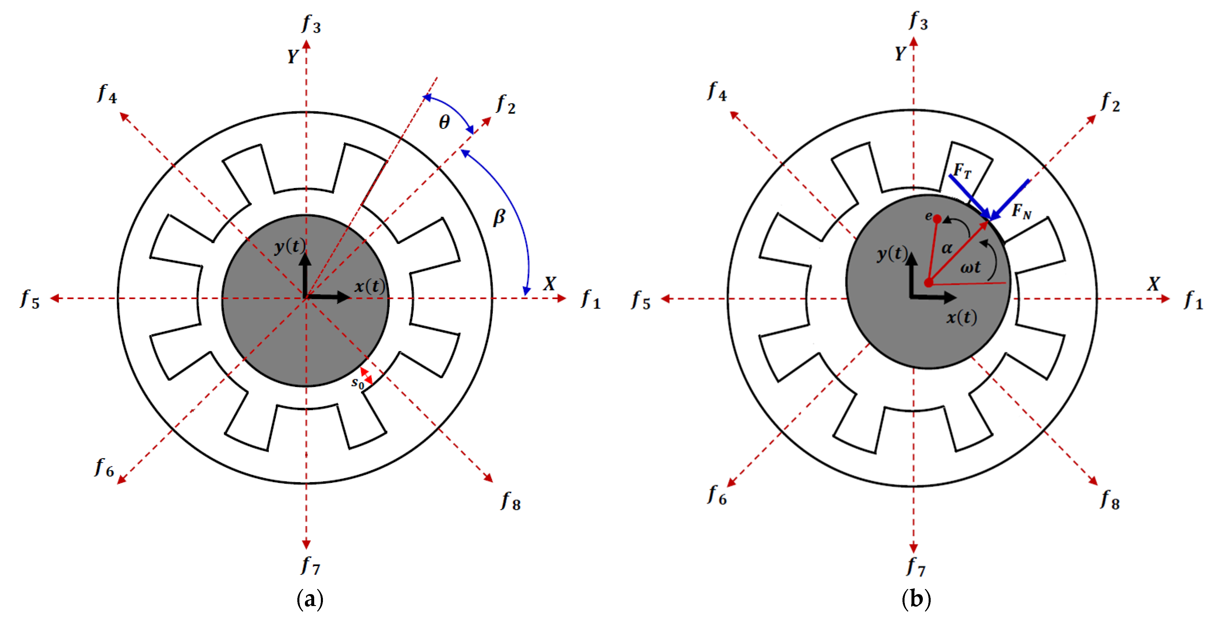
The 8-poles AMBS is depicted in Figure 1a. The system has been modeled as a rigid-body, two-degree-of-freedom system with mass $m$, disc eccentricity $e$, and rotates with the spinning speed $\omega$. The system is supported through 8 electromagnetic poles to cause the disc to rotate in its hovering position via generating the controllable magnetic restoring forces $F_{MX}$ and $F_{MY}$ in $X$ and $Y$ directions. Accordingly, the equations of motion for the system under consideration are [25]:

$$m\ddot{x}\left(t\right)=me{\omega }^2\cos (\omega t+\alpha )+F_{MX}+F_{CX},$$

(1)

$$m\ddot{y}\left(t\right)=me{\omega }^2\sin (\omega t+\alpha )+F_{MY}+F_{CY}.$$

(2)

where $x\left(t\right), \dot{x}\left(t\right), \ddot{x}\left(t\right)$ are the instantaneous position, velocity, and acceleration of disc in the $X-$direction, while $y\left(t\right), \dot{y}\left(t\right), \ddot{y}\left(t\right)$ are the instantaneous position, velocity, and acceleration of the disc in the $Y-$direction. $me{\omega }^2\cos \left(\omega t+\alpha \right)$ and $me{\omega }^2\sin \left(\omega t+\alpha \right)$ are the centrifugal force components in $X$ and $Y$ directions, respectively. When the magnetic forces $F_{MX}$ and $F_{MY}$ fail to support the rotating shaft in its hovering position due to centrifugal force ($me{\omega }^2$), the rotor may touch the stator housing as shown in Figure 1b, which results in the appearance of rub and impact forces (i.e., $F_T$ and $F_N$) on the rotor–stator interface. The rub-impact force components in $X$ and $Y$ directions are denoted as $F_{CX}$ and $F_{CY}$ as given in Equations (1) and (2).

2.1. Electromagnetic Restoring Forces $F_{MX}$ and $F_{MY}$

The attractive electromagnetic force $f_j$ between each pole and the rotating disc can be expressed according to the electromagnetic theory as follows [26]:

$$f_j=\frac{\mu A{n}^2{I}_j^2}{4H_j^2}\cos (\theta ),\hspace{1em}\hspace{1em}\hspace{1em}j=1,2,\dots ,8.$$

(3)

where $\mu$ is the magnetic permeability, $A$ is the cross-sectional area of each electromagnetic pole, $n$ is the windings number of the electric coil of each pole, $I_j$ is the electric current applied on each pole, $H_j$ is the actual air gap between the rotating disc and each pole, and $\theta$ is the half-angle of the radial electromagnetic circuit as shown in Figure 1a. It is worth mentioning that the eight poles are considered to be symmetric. Depending on Figure 1a, for small deviations $x$ and $y$ of the rotating disc, the actual air gap $H_j$ among the $j\mathrm{th}$ pole and the rotating disc can be written as follows:

$$\begin{array}{ll}{H}_j=s_0\mp x,& j=1,5,\\ H_j=s_0\mp x\cos \left(\beta \right)\mp y\cos \left(\beta \right),& j=2,6,\\ H_j=s_0\pm x\cos \left(\beta \right)\mp y\cos \left(\beta \right),& j=4,8, \\ H_j=s_0\mp y,& j=3,7\end{array}\}$$

(4)

where $s_0$ is the air-gap size between the rotor and stator when the rotating disc is in its nominal position, and $\beta ={45}^{\circ }$ is the angle between every two consecutive poles as depicted in Figure 1a. Depending on the geometry of the considered system, the electric current in the eight poles is suggested as follows:

$$\begin{array}{l}{I}_1=I_0-i_x, I_2=I_0-i_x-i_y, I_3=I_0-i_y, I_4=I_0+i_x-i_y,\\ I_5=I_0+i_x, I_6=I_0+i_x+i_y, I_7=I_0+i_y, I_8=I_0-i_x+i_y.\end{array}\}$$

(5)

where $I_0$ is a constant bias current, $i_x$ and $i_y$ are the control currents that depend on the displacements and velocities of the rotating disc in $X$ and $Y$ directions, respectively. The control currents are proposed such that:

$$i_x\left(t\right)=k_{1}x\left(t\right)+k_2\dot{x}\left(t\right), i_y\left(t\right)=k_{1}y\left(t\right)+k_2\dot{y}\left(t\right)$$

(6)

where $k_1$ and $k_2$ are two constants represent the proportional and derivative gains, respectively. Inserting Equations (4)–(6) into Equation (3), we have

$$f_1=\frac{1}{4}\mu n^{2}A\cos (\theta )\frac{I_1^2}{H_1^2}=\frac{1}{4}\mu n^{2}A\cos (\theta ){\left(\frac{I_0-i_x}{s_0-x}\right)}^2$$

(7)

$$f_2=\frac{1}{4}\mu n^{2}A\cos (\theta )\frac{I_2^2}{H_2^2}=\frac{1}{4}\mu n^{2}A\cos (\theta ){\left(\frac{I_0-i_x-i_y}{s_0-x\cos \left(\beta \right)-y\cos \left(\beta \right)}\right)}^2$$

(8)

$$f_3=\frac{1}{4}\mu n^{2}A\cos (\theta )\frac{I_3^2}{H_3^2}=\frac{1}{4}\mu n^{2}A\cos (\theta ){\left(\frac{I_0-i_y}{s_0-y}\right)}^2$$

(9)

$$f_4=\frac{1}{4}\mu n^{2}A\cos (\theta )\frac{I_4^2}{H_4^2}=\frac{1}{4}\mu n^{2}A\cos (\theta ){\left(\frac{I_0+i_x-i_y}{s_0+x\cos \left(\beta \right)-y\cos \left(\beta \right)}\right)}^2$$

(10)

$$f_5=\frac{1}{4}\mu n^{2}A\cos (\theta )\frac{I_5^2}{H_5^2}=\frac{1}{4}\mu n^{2}A\cos (\theta ){\left(\frac{I_0+i_x}{s_0+x}\right)}^2$$

(11)

$$f_6=\frac{1}{4}\mu n^{2}A\cos (\theta )\frac{I_6^2}{H_6^2}=\frac{1}{4}\mu n^{2}A\cos (\theta ){\left(\frac{I_0+i_x+i_y}{s_0+x\cos \left(\beta \right)+y\cos \left(\beta \right)}\right)}^2$$

(12)

$$f_7=\frac{1}{4}\mu n^{2}A\cos (\theta )\frac{I_7^2}{H_7^2}=\frac{1}{4}\mu n^{2}A\cos (\theta ){\left(\frac{I_0+i_y}{s_0+y}\right)}^2$$

(13)

$$f_8=\frac{1}{4}\mu n^{2}A\cos (\theta )\frac{I_8^2}{H_8^2}=\frac{1}{4}\mu n^{2}A\cos (\theta ){\left(\frac{I_0-i_x+i_y}{s_0-x\cos \left(\beta \right)+y\cos \left(\beta \right)}\right)}^2$$

(14)

Depending on the geometry of Figure 1a, the resultant restoring forces $F_{MX}$ and $F_{MY}$ as in Equations (1) and (2) can be represented as follows:

$$F_{MX}=f_1-f_5+\left(f_2+f_8-f_4-f_6\right)\cos (\beta )$$

(15)

$$F_{MY}=f_3-f_7+\left(f_2+f_4-f_6-f_8\right)\cos (\beta )$$

(16)

By expanding the nonlinear forces $f_j$ ($i=1, 2, \dots , 8$) in Equations (7)–(14) using a third-order maclurin series in terms of $x,y, i_x, i_y$, and then substituting the resulting equations into Equations (15) and (16), we have

$$\begin{array}{c}{F}_{MX}=\frac{1}{4s_0^5}\mu n^{2}A\cos (\theta )[(8{\cos }^2\left(\beta \right)s_0^2{I}_0^2-8\cos \left(\beta \right)s_0^3{I}_0{k}_1-4s_0^3{I}_0{k}_1\\ +4s_0^2{I}_0^2)x-(4s_0^3{I}_0{k}_2+8\cos (\beta )s_0^3{I}_0{k}_2)\dot{x}+(4s_0^2{k}_1^2+8I_0^2\\ +16{\cos }^4\left(\beta \right)I_0^2+8{\cos }^2\left(\beta \right)s_0^2{k}_1^2-24{\cos }^3\left(\beta \right)s_0{I}_0{k}_1-12s_0{I}_0{k}_1)x^3\\ +(24{\cos }^2\left(\beta \right)s_0^2{k}_1^2-72{\cos }^3\left(\beta \right)s_0{I}_0{k}_1+48{\cos }^4\left(\beta \right)I_0^2)x{y}^2\\ +(-24{\cos }^3\left(\beta \right)s_0{I}_0{k}_2+16{\cos }^2\left(\beta \right)s_0^2{k}_1{k}_2-12s_0{I}_0{k}_2+8s_0^2{k}_1{k}_2)x^2\dot{x}\\ +(4s_0^2{k}_2^2+8{\cos }^2\left(\beta \right)s_0^2{k}_2^2)x{\dot{x}}^2+(32{\cos }^2\left(\beta \right)s_0^2{k}_1{k}_2\\ -48{\cos }^3\left(\beta \right)s_0{I}_0{k}_2)xy\dot{y}+8{\cos }^2\left(\beta \right)s_0^2{k}_2^{2}x{\dot{y}}^2\\ +16{\cos }^2\left(\beta \right)s_0^2{k}_2^2\dot{x}y\dot{y}+(16{\cos }^2\left(\beta \right)s_0^2{k}_1{k}_2-24{\cos }^3\left(\beta \right)s_0{I}_0{k}_2)\dot{x}{y}^2]\end{array}$$

(17)

$$\begin{array}{c}{F}_{MY}=\frac{1}{4s_0^5}\mu n^{2}A\cos (\theta )[(8{\cos }^2\left(\beta \right)s_0^2{I}_0^2-8\cos \left(\beta \right)s_0^3{I}_0{k}_1-4s_0^3{I}_0{k}_1\\ +4s_0^2{I}_0^2)y-(4s_0^3{I}_0{k}_2+8\cos \left(\beta \right)s_0^3{I}_0{k}_2)\dot{y}+(4s_0^2{k}_1^2+8I_0^2\\ +16{\cos }^4\left(\beta \right)I_0^2+8{\cos }^2\left(\beta \right)s_0^2{k}_1^2-24{\cos }^3\left(\beta \right)s_0{I}_0{k}_1-12s_0{I}_0{k}_1)y^3\\ +(24{\cos }^2\left(\beta \right)s_0^2{k}_1^2-72{\cos }^3\left(\beta \right)s_0{I}_0{k}_1+48{\cos }^4\left(\beta \right)I_0^2)y{x}^2\\ +(-24{\cos }^3\left(\beta \right)s_0{I}_0{k}_2+16{\cos }^2\left(\beta \right)s_0^2{k}_1{k}_2-12s_0{I}_0{k}_2+8s_0^2{k}_1{k}_2)y^2\dot{y}\\ +(4s_0^2{k}_2^2+8{\cos }^2\left(\beta \right)s_0^2{k}_2^2)y{\dot{y}}^2+(32{\cos }^2\left(\beta \right)s_0^2{k}_1{k}_2\\ -48{\cos }^3\left(\beta \right)s_0{I}_0{k}_2)yx\dot{x}+8{\cos }^2\left(\beta \right)s_0^2{k}_2^{2}y{\dot{x}}^2+16{\cos }^2\left(\beta \right)s_0^2{k}_2^2\dot{y}x\dot{x}\\ +(16{\cos }^2\left(\beta \right)s_0^2{k}_1{k}_2-24{\cos }^3\left(\beta \right)s_0{I}_0{k}_2)\dot{y}{x}^2]\end{array}$$

(18)

2.2. Rub and Impact Forces $F_{CX}$ and $F_{CY}$

The rotor AMBS disc is constrained within the electromagnetic poles’ housing. Therefore, if the rotating disc oscillates with instantaneous radial displacement $R\left(t\right)=\sqrt{x{\left(t\right)}^2+y{\left(t\right)}^2}$ that is larger than the nominal air gap $s_0$ (i.e., when $R\left(t\right)\ge s_0$) as illustrated in Figure 1b, contact between the rotating disc and the pole leg should occur. The occurrence of this contact results in both impact force ($F_N$) and rub force ($F_T$) on the rotor–stator interface. Accordingly, the rub and impact forces can be expressed as follows [27,28,29,30]:

$$F_N\left(t\right)=k(R-s_0) H(R-s_0),$$

(19)

$$F_T={\mu }_f{F}_N={\mu }_{f}k(R-s_0)H(R-s_0).$$

(20)

where $k$ is the impact stiffness coefficient between the rotor and the pole leg, ${\mu }_f$ is the dynamic friction coefficient between the rotating disc and poles, and $H$ is the Heaviside function. Based on the geometry of Figure 1b, the resultant components of the rub and impact forces in $X$ and $Y$ directions can be written as follows:

$$F_{CX}=-F_T\sin (\omega t)-F_N\cos (\omega t)=\frac{k}{R}(R-s_0)({\mu }_{f}y-x) H(R-s_0)$$

(21)

$$F_{CY}=-F_T\cos (\upsilon t)-F_N\sin (\upsilon t)=-\frac{k}{R}(R-s_0)({\mu }_{f}x+y) H(R-s_0).$$

(22)

where $\cos \left(\omega t\right)=\frac{x}{R}, \sin \left(\omega t\right)=\frac{y}{R}$ as it is clear from Figure 1b.

2.3. The Rotor System Equations of Motion

Substituting Equations (17), (18), (21) and (22) into Equations (1) and (2), with the introduction of the dimensionless quantities $u=\frac{x}{s_0}, v=\frac{y}{s_0}$, $r=\sqrt{u^2+v^2}=\sqrt{{\left(\frac{x}{s_0}\right)}^2+{\left(\frac{y}{s_0}\right)}^2}=\frac{R}{s_0}$, $\tau ={\omega }_{n}t$, $\dot{u}=\dot{\frac{x}{{\omega }_n{s}_0}}, \dot{v}=\dot{\frac{y}{{\omega }_n{s}_0}},$ $\ddot{u}=\frac{\ddot{x}}{{\omega }_n^2{s}_0}, \ddot{v}=\frac{\ddot{y}}{{\omega }_n^2{s}_0},$ ${\delta }_1=\frac{s_0}{I_0}{k}_1, {\delta }_2=\frac{s_0{\omega }_n}{I_0}{k}_2,$ $\lambda =\frac{k}{m{\omega }_n^2},E=\frac{e}{s_0}, \mathsf{\Omega }=\frac{\omega }{{\omega }_n}$, and ${\omega }_n=\sqrt{\frac{\mu I_0^2{n}^{2}Acos\left(\theta \right)}{4m{s}_0^3}}$, the following normalized equations of motion can be obtained:

$$\begin{array}{l}\frac{d^{2}u}{d{\tau }^2}+{\mu }_s\frac{du}{d\tau }+{\omega }_s^{2}u+{\eta }_1{u}^3+{\eta }_{2}u{v}^2+{\eta }_3{u}^2\frac{du}{d\tau }+{\eta }_{4}u{\left(\frac{du}{d\tau }\right)}^2+{\eta }_{5}uv\frac{dv}{d\tau }\\ +{\eta }_{6}u{\left(\frac{dv}{d\tau }\right)}^2+{\eta }_{7}v\left(\frac{du}{d\tau }\right)\left(\frac{dv}{d\tau }\right)+{\eta }_8{v}^2\frac{du}{d\tau }=E{\mathsf{\Omega }}^2\cos (\mathsf{\Omega }\tau +\alpha ) \\ +\frac{\lambda }{r}(r-1)({\mu }_{f}v-u)H(r-1),\end{array}$$

(23)

$$\begin{array}{l}\frac{d^{2}v}{d{\tau }^2}+{\mu }_s\frac{dv}{d\tau }+{\omega }_s^{2}v+{\eta }_1{v}^3+{\eta }_{2}v{u}^2+{\eta }_3{v}^2\frac{dv}{d\tau }+{\eta }_{4}v{\left(\frac{dv}{d\tau }\right)}^2+{\eta }_{5}vu\frac{du}{d\tau }\\ +{\eta }_{6}v{\left(\frac{du}{d\tau }\right)}^2+{\eta }_{7}u\left(\frac{du}{d\tau }\right)\left(\frac{dv}{d\tau }\right)+{\eta }_8{u}^2\frac{dv}{d\tau }=E{\mathsf{\Omega }}^2\sin (\mathsf{\Omega }\tau +\alpha ) \\ -\frac{\lambda }{r}(r-1)({\mu }_{f}u+v) H(r-1).\end{array}$$

(24)

where the system parameters ${\mu }_s, {\omega }_s^2, {\eta }_{j }, \left(j=1,2,\dots ,8\right)$ are given in Appendix A. It is important to notice that the introduced normalized coordinates $u=\frac{x}{s_0}$ and $v=\frac{y}{s_0}$ are the ratio of the instantaneous displacements $x\left(t\right)$ and $y\left(t\right)$ to the air-gap size $s_0$. Accordingly, if $\left|u\left(\tau \right)\right|<1$ and $\left|v\left(\tau \right)\right|<1$, the rotating disc vibrated without rub and/or impact between the disc and the pole legs. However, if $\left|u\left(\tau \right)\right|\ge 1$ and/or $\left|v\left(\tau \right)\right|\ge 1$, the rub-impact force appears on the rotor–stator interface. So, the derived equations of motion (i.e., Equations (23) and (24)) are analyzed in two stages. Firstly, the rotor AMBS is investigated as a continuous dynamical system when omitting the rub and impact forces via setting the impact stiffness coefficient $\lambda =\frac{k}{m{\omega }_n^2}=0$ in order to determine the conditions at which the rub and/or the impact occurs. Secondly, utilizing the Poincare map, bifurcation diagram, and frequency spectrum, the entire system is numerically explored to investigate system oscillations when the rub and/or impact forces are assured.

3. Periodic Solution and Amplitude-Phase Modulating Equations of the Continuous System

Utilizing the multiple time scales method, the periodic solution of the considered system when the rub-impact force is omitted (i.e., $\lambda =0$) can be proposed as follows [31]:

$$u\left(\tau \right)=u_1(T_0,T_1)+\epsilon u_2(T_0,T_1)+O\left({\epsilon }^2\right)$$

(25)

$$v\left(\tau \right)=v_1(T_0,T_1)+\epsilon v_2(T_0,T_1)+O\left({\epsilon }^2\right)$$

(26)

In terms of $T_0=\tau$ and $T_1=ϵ\tau$, the time derivatives are transformed to:

$$\frac{d}{d\tau }=D_0+\epsilon D_1, \frac{d^2}{d{\tau }^2}=D_0^2+2\epsilon D_0{D}_1,D_j=\frac{\partial }{\partial T_j}, j=0,1$$

(27)

Accordingly, the system parameters can be scaled as follows:

$${\mu }_s=\epsilon {\widehat{\mu }}_s, E=\epsilon \widehat{E}, {\eta }_j=\epsilon {\widehat{\eta }}_j, j=1,2,\dots ,8.$$

(28)

Substituting Equations (25)–(28) into Equations (23) and (24) while comparing the coefficients of ${\epsilon }^0$ and ${\epsilon }^1$, we have

$O\left({\epsilon }^0\right):$

$$(D_0^2+{\omega }_s^2)u_1=0$$

(29)

$$(D_0^2+{\omega }_s^2)v_1=0$$

(30)

$O\left({\epsilon }^1\right):$

$$\begin{array}{c}(D_0^2+{\omega }_s^2)u_2=-2D_0{D}_1{u}_1-{\widehat{\mu }}_s{D}_0{u}_1-{\widehat{\eta }}_1{u}_1^3-{\eta }_2{u}_1{v}_1^2-{\eta }_3{u}_1^2\left(D_0{u}_1\right)\\ -{\eta }_4{u}_1{\left(D_0{u}_1\right)}^2-{\eta }_5{u}_1{v}_1\left(D_0{v}_1\right)-{\widehat{\eta }}_6{u}_1{\left(D_0{v}_1\right)}^2\\ \hspace{1em}\hspace{1em}\hspace{1em}\hspace{1em}\hspace{1em} -{\eta }_7\left(D_0{u}_1\right)v_1\left(D_0{v}_1\right)-{\widehat{\eta }}_8\left(D_0{u}_1\right)v_1^2+\widehat{E}{\mathsf{\Omega }}^2\cos (\mathsf{\Omega }\tau +\alpha ) \end{array}$$

(31)

$$\begin{array}{c}(D_0^2+{\omega }_s^2)v_2=-2D_0{D}_1{v}_1-{\widehat{\mu }}_s{D}_0{v}_1-{\widehat{\eta }}_1{v}_1^3-{\eta }_2{v}_1{u}_1^2-{\eta }_3{v}_1^2\left(D_0{v}_1\right)\\ -{\eta }_4{v}_1{\left(D_0{v}_1\right)}^2-{\eta }_5{v}_1{u}_1\left(D_0{u}_1\right)-{\widehat{\eta }}_6{v}_1{\left(D_0{u}_1\right)}^2\\ \hspace{1em}\hspace{1em}\hspace{1em}\hspace{1em}\hspace{1em} -{\eta }_7\left(D_0{v}_1\right)u_1\left(D_0{u}_1\right)-{\widehat{\eta }}_8\left(D_0{v}_1\right)u_1^2+\widehat{E}{\mathsf{\Omega }}^2\sin (\mathsf{\Omega }\tau +\alpha )\end{array}$$

(32)

The solutions of Equations (29) and (30) can be written in the following form:

$$u_1(T_0,T_1)=A_1\left(T_1\right)e^{i{\omega }_s{T}_0}+\overline{A_1}\left(T_1\right)e^{-i{\omega }_s{T}_0}$$

(33)

$$v_1(T_0,T_1)=A_2\left(T_1\right)e^{i{\omega }_s{T}_0}+\overline{A_2}\left(T_1\right)e^{-i{\omega }_s{T}_0}$$

(34)

where the coefficients $A_j\left(T_1\right)$ {$j$ = 1, 2} are two unknown functions of $T_1$ up to this stage of the analysis, while $\overline{A_j}\left(T_1\right)$ are the complex conjugate of $A_j\left(T_1\right)$. Substituting Equations (33) and (34) into Equations (31) and (32), we can conclude the primary resonance case ($\mathsf{\Omega }\cong {\omega }_s$) with 1:1 internal resonance. We introduce the detuning parameter $\sigma$ to describe the closeness of the disc spinning-speed $\mathsf{\Omega }$ to the system natural frequency ${\omega }_s$ as follows:

$$\mathsf{\Omega }={\omega }_s+\sigma ={\omega }_s+\epsilon \widehat{\sigma },?$$

(35)

Inserting Equations (33), (34), and (35) into Equations (31) and (32), we get the solvability conditions of Equations (31) and (32) as follows:

$$\begin{array}{l}-2i{\omega }_s\frac{d}{d{T}_1}{A}_1\left(T_1\right)-i{\widehat{\mu }}_s{\omega }_s{A}_1\left(T_1\right)-3{\widehat{\eta }}_1{A}_1^2\left(T_1\right){\overline{A}}_1\left(T_1\right)\\ -2{\eta }_2{A}_1\left(T\right)A_2\left(T_1\right){\overline{A}}_2\left(T_1\right)-{\eta }_2{\overline{A}}_1\left(T_1\right)A_2^2\left(T_1\right)-i{\eta }_3{\omega }_s{A}_1^2\left(T_1\right){\overline{A}}_1\left(T_1\right)\\ -{\widehat{\eta }}_4{\omega }_s^2{A}_1^2\left(T\right){\overline{A}}_1\left(T_1\right)-i{\eta }_5{\omega }_s{\overline{A}}_1\left(T_1\right)A_2^2\left(T\right)-2{\eta }_6{\omega }_s^2{A}_1\left(T_1\right)A_2\left(T_1\right){\overline{A}}_2\left(T_1\right)\\ +{\widehat{\eta }}_6{\omega }_s^2{\overline{A}}_1\left(T_1\right)A_2^2\left(T_1\right)-{\widehat{\eta }}_7{\omega }_s^2{\overline{A}}_1\left(T_1\right)A_2^2\left(T_1\right)-2i{\eta }_8{\omega }_s{A}_1\left(T_1\right)A_2\left(T_1\right){\overline{A}}_2\left(T_1\right)\\ +i{\widehat{\eta }}_8{\omega }_s{\overline{A}}_1\left(T_1\right)A_2^2\left(T_1\right)+\frac{1}{2}F{\mathsf{\Omega }}^2{e}^{i(\widehat{\sigma }{T}_1+\alpha )}=0, \end{array}$$

(36)

$$\begin{array}{l}-2i{\omega }_s\frac{d}{d{T}_1}{A}_2\left(T_1\right)-i{\widehat{\mu }}_s{\omega }_s{A}_2\left(T_1\right)-3{\widehat{\eta }}_1{A}_2^2\left(T_1\right){\overline{A}}_2\left(T_1\right)-2{\eta }_2{A}_2\left(T\right)A_1\left(T_1\right){\overline{A}}_1\left(T_1\right)\\ -{\eta }_2{\overline{A}}_2\left(T_1\right)A_1^2\left(T_1\right)-i{\eta }_3{\omega }_s{A}_2^2\left(T_1\right){\overline{A}}_2\left(T_1\right)-{\widehat{\eta }}_4{\omega }_s^2{A}_2^2\left(T\right){\overline{A}}_2\left(T_1\right)\\ -i{\eta }_5{\omega }_s{\overline{A}}_2\left(T_1\right)A_1^2\left(T\right)-2{\eta }_6{\omega }_s^2{A}_2\left(T_1\right)A_1\left(T_1\right){\overline{A}}_1\left(T_1\right)+{\widehat{\eta }}_6{\omega }_s^2{\overline{A}}_2\left(T_1\right)A_1^2\left(T_1\right)\\ -{\widehat{\eta }}_7{\omega }_s^2{\overline{A}}_2\left(T_1\right)A_1^2\left(T_1\right)-2i{\eta }_8{\omega }_s{A}_2\left(T_1\right)A_1\left(T_1\right){\overline{A}}_1\left(T_1\right)+i{\widehat{\eta }}_8{\omega }_s{\overline{A}}_2\left(T_1\right)A_1^2\left(T_1\right)\\ -\frac{1}{2}iF{\mathsf{\Omega }}^2{e}^{i(\widehat{\sigma }{T}_1+\alpha )}=0.\end{array}$$

(37)

By replacing the functions $A_j\left(T_1\right)=\frac{a_j}{2}{e}^{i{\theta }_j} \left\{j=1, 2\right\}$ into Equations (36) and (37) while restoring the system parameters to their original form (i.e.,$T_1=ϵ\tau , {\widehat{\mu }}_s=\frac{\mu }{ϵ}, \widehat{E}=\frac{E}{ϵ}, {\widehat{\eta }}_j=\frac{{\eta }_j}{ϵ}, j=1,2,\dots ,8)$, we can obtain the following amplitude-phase modulating equations:

$$\begin{array}{c}\frac{d}{d\tau }{a}_1=F_1(a_1,a_2,{\gamma }_1,{\gamma }_2)=-\frac{1}{2}{\mu }_s{a}_1+\frac{1}{8\omega }{\eta }_2{a}_1{a}_2^2\sin (2{\gamma }_1-2{\gamma }_2)-\frac{1}{8}{\eta }_3{a}_1^3\\ \hspace{1em}\hspace{1em} -\frac{1}{8}{\eta }_5{a}_1{a}_2^2\cos (2{\gamma }_1-2{\gamma }_2)-\frac{1}{8}{\eta }_6{\omega }_s{a}_1{a}_2^2\sin (2{\gamma }_1-2{\gamma }_2)\\ \hspace{1em}\hspace{1em} +\frac{1}{8}{\eta }_7{\omega }_s{a}_1{a}_2^2\sin (2{\gamma }_1-2{\gamma }_2)-\frac{1}{4}{\eta }_8{a}_1{a}_2^2+\frac{1}{8}{\eta }_8{a}_1{a}_2^2\cos (2{\gamma }_1-2{\gamma }_2)\\ \hspace{1em}\hspace{1em} -\frac{1}{2{\omega }_s}E{\mathsf{\Omega }}^2\sin \left({\gamma }_1\right)\end{array}$$

(38)

$$\begin{array}{c}\frac{d}{d\tau }{a}_2=F_2(a_1,a_2,{\gamma }_1,{\gamma }_2)=-\frac{1}{2}{\mu }_s{a}_2-\frac{1}{8{\omega }_s}{\eta }_2{a}_2{a}_1^2\sin (2{\gamma }_1-2{\gamma }_2)-\frac{1}{8}{\eta }_3{a}_2^3\\ \hspace{1em}\hspace{1em} -\frac{1}{8}{\eta }_5{a}_2{a}_1^2\cos (2{\gamma }_1-2{\gamma }_2)+\frac{1}{8}{\eta }_6{\omega }_s{a}_2{a}_1^2\sin (2{\gamma }_1-2{\gamma }_2)\\ \hspace{1em}\hspace{1em} -\frac{1}{8}{\eta }_7{\omega }_s{a}_2{a}_1^2\sin (2{\gamma }_1-2{\gamma }_2)-\frac{1}{4}{\eta }_8{a}_2{a}_1^2+\frac{1}{8}{\eta }_8{a}_2{a}_1^2\cos (2{\gamma }_1-2{\gamma }_2)\\ \hspace{1em}\hspace{1em} -\frac{1}{2{\omega }_s}E{\mathsf{\Omega }}^2\cos \left({\gamma }_2\right)\end{array}$$

(39)

$$\begin{array}{c}\frac{d}{d\tau }{\gamma }_1=F_3(a_1,a_2,{\gamma }_1,{\gamma }_2)=-\sigma +\frac{3}{8{\omega }_s}{\eta }_1{a}_1^2+\frac{1}{8{\omega }_s}{\eta }_2{a}_2^2\cos (2{\gamma }_1-2{\gamma }_2)\\ \hspace{1em}\hspace{1em} +\frac{1}{4{\omega }_s}{\eta }_2{a}_2^2+\frac{1}{8}{\eta }_4{\omega }_s{a}_1^2+\frac{1}{8}{\eta }_5{a}_2^2\sin (2{\gamma }_1-2{\gamma }_2)\\ \hspace{1em}\hspace{1em} -\frac{1}{8}{\eta }_6{\omega }_s{a}_2^2\cos (2{\gamma }_1-2{\gamma }_2)+\frac{1}{4}{\eta }_6{\omega }_s{a}_2^2+\frac{1}{8}{\eta }_7{\omega }_s{a}_2^2\cos (2{\gamma }_1-2{\gamma }_2)\\ \hspace{1em}\hspace{1em} -\frac{1}{8}{\eta }_8{a}_2^2\sin (2{\gamma }_1-2{\gamma }_2)-\frac{1}{2{\omega }_s{a}_1}E{\mathsf{\Omega }}^2\cos \left({\gamma }_1\right)\end{array}$$

(40)

$$\begin{array}{c}\frac{d}{d\tau }{\gamma }_2=F_4(a_1,a_2,{\gamma }_1,{\gamma }_2)=-\sigma +\frac{3}{8{\omega }_s}{\eta }_1{a}_2^2+\frac{1}{8{\omega }_s}{\eta }_2{a}_1^2\cos (2{\gamma }_1-2{\gamma }_2)\\ \hspace{1em}\hspace{1em} +\frac{1}{4{\omega }_s}{\eta }_2{a}_1^2+\frac{1}{8}{\eta }_4{\omega }_s{a}_2^2-\frac{1}{8}{\eta }_5{a}_1^2\sin (2{\gamma }_1-2{\gamma }_2)\\ \hspace{1em}\hspace{1em} -\frac{1}{8}{\eta }_6{\omega }_s{a}_1^2\cos (2{\gamma }_1-2{\gamma }_2)+\frac{1}{4}{\eta }_6{\omega }_s{a}_1^2+\frac{1}{8}{\eta }_7{\omega }_s{a}_1^2\cos (2{\gamma }_1-2{\gamma }_2)\\ \hspace{1em}\hspace{1em} +\frac{1}{8}{\eta }_8{a}_1^2\sin (2{\gamma }_1-2{\gamma }_2)+\frac{1}{2{\omega }_s{a}_2}E{\mathsf{\Omega }}^2\sin \left({\gamma }_2\right)\end{array}$$

(41)

where ${\gamma }_1={\theta }_1-\sigma \tau -\alpha , {\gamma }_2={\theta }_2-\sigma \tau -\alpha$. Substituting Equations (33) and (34) into Equations (25) and (26) with replacing $A_j\left(T_1\right)=\frac{a_j}{2}{e}^{i{\theta }_j}$ $\left\{j=1, 2\right\}$, we can obtain the following periodic solution of the system’s original equations (i.e., Equations (23) and (24)) when $\lambda =0$ as follows:

$$u\left(\tau \right)=a_1\left(\tau \right)\cos (\mathsf{\Omega }\tau +{\gamma }_1)$$

(42)

$$v\left(\tau \right)=a_2\left(\tau \right)\cos (\mathsf{\Omega }\tau +{\gamma }_2)$$

(43)

According to Equations (42) and (43), the functions $a_1\left(\tau \right), a_2\left(\tau \right)$ represent the vibration amplitudes of the rotor AMBS system when $\lambda =0$ in $X$ and $Y$ directions, respectively, and ${\gamma }_1\left(\tau \right)$, ${\gamma }_2\left(\tau \right)$ denote the phase-angles of the system motion. These functions $a_1\left(\tau \right)$, $a_2\left(\tau \right)$,${\gamma }_1\left(\tau \right)$, and ${\gamma }_2\left(\tau \right)$ are governed by the nonlinear autonomous dynamical system given by Equations (38)–(41). Accordingly, setting $\frac{d{a}_1}{d\tau }=\frac{d{a}_2}{d\tau }=\frac{d{\gamma }_1}{d\tau }=\frac{d{\gamma }_2}{d\tau }=0$ into Equations (38)–(41), we get the following nonlinear system of algebraic equations:

$$\begin{array}{l}-\frac{1}{2}{\mu }_s{a}_1+\frac{1}{8\omega }{\eta }_2{a}_1{a}_2^2\sin (2{\gamma }_1-2{\gamma }_2)-\frac{1}{8}{\eta }_3{a}_1^3-\frac{1}{8}{\eta }_5{a}_1{a}_2^2\cos (2{\gamma }_1-2{\gamma }_2)\\ -\frac{1}{8}{\eta }_6{\omega }_s{a}_1{a}_2^2\sin (2{\gamma }_1-2{\gamma }_2)+\frac{1}{8}{\eta }_7{\omega }_s{a}_1{a}_2^2\sin (2{\gamma }_1-2{\gamma }_2)-\frac{1}{4}{\eta }_8{a}_1{a}_2^2\\ +\frac{1}{8}{\eta }_8{a}_1{a}_2^2\cos (2{\gamma }_1-2{\gamma }_2)-\frac{1}{2{\omega }_s}E{\mathsf{\Omega }}^2\sin \left({\gamma }_1\right)=0\end{array}$$

(44)

$$\begin{array}{l}-\frac{1}{2}{\mu }_s{a}_2-\frac{1}{8\omega }{\eta }_2{a}_2{a}_1^2\sin (2{\gamma }_1-2{\gamma }_2)-\frac{1}{8}{\eta }_3{a}_2^3-\frac{1}{8}{\eta }_5{a}_2{a}_1^2\cos (2{\gamma }_1-2{\gamma }_2)\\ +\frac{1}{8}{\eta }_6{\omega }_s{a}_2{a}_1^2\sin (2{\gamma }_1-2{\gamma }_2)-\frac{1}{8}{\eta }_7{\omega }_s{a}_2{a}_1^2\sin (2{\gamma }_1-2{\gamma }_2)-\frac{1}{4}{\eta }_8{a}_2{a}_1^2\\ +\frac{1}{8}{\eta }_8{a}_2{a}_1^2\cos (2{\gamma }_1-2{\gamma }_2)-\frac{1}{2{\omega }_s}E{\mathsf{\Omega }}^2\cos \left({\gamma }_2\right)=0\end{array}$$

(45)

$$\begin{array}{l}-\sigma +\frac{3}{8{\omega }_s}{\eta }_1{a}_1^2+\frac{1}{8{\omega }_s}{\eta }_2{a}_2^2\cos (2{\gamma }_1-2{\gamma }_2)+\frac{1}{4{\omega }_s}{\eta }_2{a}_2^2+\frac{1}{8}{\eta }_4{\omega }_s{a}_1^2\\ +\frac{1}{8}{\eta }_5{a}_2^2\sin (2{\gamma }_1-2{\gamma }_2)-\frac{1}{8}{\eta }_6{\omega }_s{a}_2^2\cos (2{\gamma }_1-2{\gamma }_2)+\frac{1}{4}{\eta }_6{\omega }_s{a}_2^2\\ +\frac{1}{8}{\eta }_7{\omega }_s{a}_2^2\cos (2{\gamma }_1-2{\gamma }_2)-\frac{1}{8}{\eta }_8{a}_2^2\sin (2{\gamma }_1-2{\gamma }_2)\\ -\frac{1}{2{\omega }_s{a}_1}E{\mathsf{\Omega }}^2\cos \left({\gamma }_1\right)=0\end{array}$$

(46)

$$\begin{array}{l}-\sigma +\frac{3}{8{\omega }_s}{\eta }_1{a}_2^2+\frac{1}{8{\omega }_s}{\eta }_2{a}_1^2\cos (2{\gamma }_1-2{\gamma }_2)+\frac{1}{4{\omega }_s}{\eta }_2{a}_1^2+\frac{1}{8}{\eta }_4{\omega }_s{a}_2^2\\ -\frac{1}{8}{\eta }_5{a}_1^2\sin (2{\gamma }_1-2{\gamma }_2)-\frac{1}{8}{\eta }_6{\omega }_s{a}_1^2\cos (2{\gamma }_1-2{\gamma }_2)+\frac{1}{4}{\eta }_6{\omega }_s{a}_1^2\\ +\frac{1}{8}{\eta }_7{\omega }_s{a}_1^2\cos (2{\gamma }_1-2{\gamma }_2)+\frac{1}{8}{\eta }_8{a}_1^2\sin (2{\gamma }_1-2{\gamma }_2)\\ +\frac{1}{2{\omega }_s{a}_2}E{\mathsf{\Omega }}^2\sin \left({\gamma }_2\right)=0\end{array}$$

(47)

By solving Equations (44)–(47) in terms of the system and control parameters (i.e., $\sigma ,E, {\delta }_1, {\delta }_2$), we can obtain the different response curves as illustrated in Section 4. Furthermore, the stability of the solution of Equations (44)–(47) can be explored via investigating the Jacobian matrix eigenvalues of the right-hand side of Equations (38)–(41). Let the steady-state solution of Equations (44)–(47) be ($a_{10}, a_{20},{\gamma }_{10},$ ${\gamma }_{20}$), while ($a_{11}, a_{21},{\gamma }_{11},$ ${\gamma }_{21}$) is a small perturbation about that steady-state solution. Accordingly, we can assume

$$\begin{array}{l}{a}_1=a_{10}+a_{11}, a_2=a_{20}+a_{21}, {\gamma }_1={\gamma }_{10}+{\gamma }_{11}, {\gamma }_2={\gamma }_{20}+{\gamma }_{21}\\ \Rightarrow \frac{d{a}_1}{d\tau }=\frac{d{a}_{11}}{d\tau }, \frac{d{a}_2}{d\tau }=\frac{d{a}_{21}}{d\tau }, \frac{d{\gamma }_1}{d\tau }=\frac{d{\gamma }_{11}}{d\tau }, \frac{d{\gamma }_2}{d\tau }=\frac{d{\gamma }_{21}}{d\tau }\end{array}\}$$

(48)

Substituting Equation (48) into Equations (38)–(41), we can obtain the following linearized model about the equilibrium point ($a_{10}, a_{20},{\gamma }_{10},$ ${\gamma }_{20}$) as:

$$\left[\begin{array}{c}\frac{d{a}_{11}}{d\tau }\\ \frac{d{a}_{21}}{d\tau }\\ \frac{d{\gamma }_{11}}{d\tau }\\ \frac{d{\gamma }_{21}}{d\tau }\end{array}\right]=\left[\begin{array}{cccc}\frac{\partial F_1}{\partial a_{11}}& \frac{\partial F_1}{\partial a_{21}}& \frac{\partial F_1}{\partial {\gamma }_{11}}& \frac{\partial F_1}{\partial {\gamma }_{21}}\\ \frac{\partial F_2}{\partial a_{11}}& \frac{\partial F_2}{\partial a_{21}}& \frac{\partial F_2}{\partial {\gamma }_{11}}& \frac{\partial F_2}{\partial {\gamma }_{21}}\\ \frac{\partial F_3}{\partial a_{11}}& \frac{\partial F_3}{\partial a_{21}}& \frac{\partial F_3}{\partial {\gamma }_{11}}& \frac{\partial F_3}{\partial {\gamma }_{21}}\\ \frac{\partial F_4}{\partial a_{11}}& \frac{\partial F_4}{\partial a_{21}}& \frac{\partial F_4}{\partial {\gamma }_{11}}& \frac{\partial F_4}{\partial {\gamma }_{21}}\end{array}\right]\left[\begin{array}{c}{a}_{11}\\ a_{21}\\ {\gamma }_{11}\\ {\gamma }_{21}\end{array}\right]$$

(49)

where the coefficients of the above Jacobian matrix are given in the Appendix B. Accordingly, the steady-state solutions of the autonomous system (Equations (38)–(41)) can be given via solving the nonlinear algebraic equations (Equations (44)–(47)). Additionally, the stability of that solution can be investigated via exploring the eigenvalues of the Jacobian matrix.

4. Oscillatory Behaviors of the Rotor System with and without Rub-Impact Force

According to the periodic solutions given by Equations (42) and (43), it is easy to show that the rotor system can oscillate without rub-impact force occurrence if $\left|u\left(\tau \right)\right|=\left|a_1\left(\tau \right)\cos \left(\mathsf{\Omega }\tau +{\gamma }_1\right)\right|<1$ and $\left|v\left(\tau \right)\right|=\left|a_2\left(\tau \right)\cos \left(\mathsf{\Omega }\tau +{\gamma }_2\right)\right|<1$. This implies that as long $a_1<1$ and $a_2<1$, there is no rub-impact force between the rotor and the stator, otherwise (i.e., if $a_1\ge 1$ and/or $a_2\ge 1$) the rub-impact force between the rotor and stator occurs. Accordingly, the steady-state oscillations of the considered system can be investigated via solving the nonlinear algebraic system given by Equations (44)–(47) numerically in terms of the system parameters $\sigma ,E, {\delta }_1,$ and ${\delta }_2$ as long as $a_1<1$ and $a_2<1$. In addition, the solution stability of Equations (44)–(47) can be explored via examining the eigenvalues of the linearized system given by Equation (49). However, if $a_1\ge 1$ and/or $a_2\ge 1$, this means there is the occurrence of the rub and/or impact forces, which necessitates the investigation of the whole discontinuous system given by Equations (23) and (24) numerically when $\lambda \ne 0$. The different response curves and bifurcation diagrams are obtained via adopting the actual and the corresponding dimensionless parameters given in

Table 1. Rotor AMBS parameters.

Physical Parameters		Dimensionless Parameters
Rotor radius	$R=0.15 \mathrm{m}$	$E$	$0.025$
Rotor thickness	$d=0.015 \mathrm{m}$	$\alpha$	$0.0$
Rotor mass	$m=8 \mathrm{kg}$	$\lambda$	$5.0$
Rotor eccentricity	$e=1.25\times {10}^{-4} \mathrm{m}$	${\mu }_f$	$0.2$
The angle between the poles ($\beta$)	$\beta ={45}^{\circ }$	$\mathsf{\Omega }$	${\omega }_s+\sigma$
Air-gap size	$s_0=5\times {10}^{-3 }\mathrm{m}$	${\delta }_1$	$0.9$
Effective cross-sectional area of the pole	$A\cos \theta =7.44\times {10}^{-4} {\mathrm{m}}^2$	${\delta }_2$	$0.008$
turn-numbers of each coil	$n=1000$
Bias current	$I_0=2 \mathrm{A}$
Magnetic permeability	$\mu =4\pi \times {10}^{-7} {\mathrm{NA}}^{-2}$
Impact stiffness coefficient	$k=3.7397\times {10}^4 \mathrm{N}·{\mathrm{m}}^{-1}$
Proportional gain	$k_1=360 \mathrm{A}/\mathrm{m}$
Velocity gain	$k_2=0.105 \mathrm{A}·\mathrm{S}/\mathrm{m}$
The constant ${\omega }_n$	${\omega }_n=\sqrt{\frac{\mu I_0^2{n}^{2}Acos\left(\theta \right)}{4m{s}_0^3}}=30.58$

(See Refs. [21,27]). By solving Equations (44)–(47) using MATLAB software, one can obtain the different response curves as in Figure 2 where the stable solution is shown by the solid line, while the unstable solution is represented by the dotted line. To confirm the accuracy of the obtained response curves, Equations (23) and (24) (when $\lambda =0$) has been integrated numerically using the ODE45 MATLAB function. The obtained numerical results are illustrated as small circles (when sweeping the bifurcation parameters forward) and as big dots (when sweeping the bifurcation parameters backward).

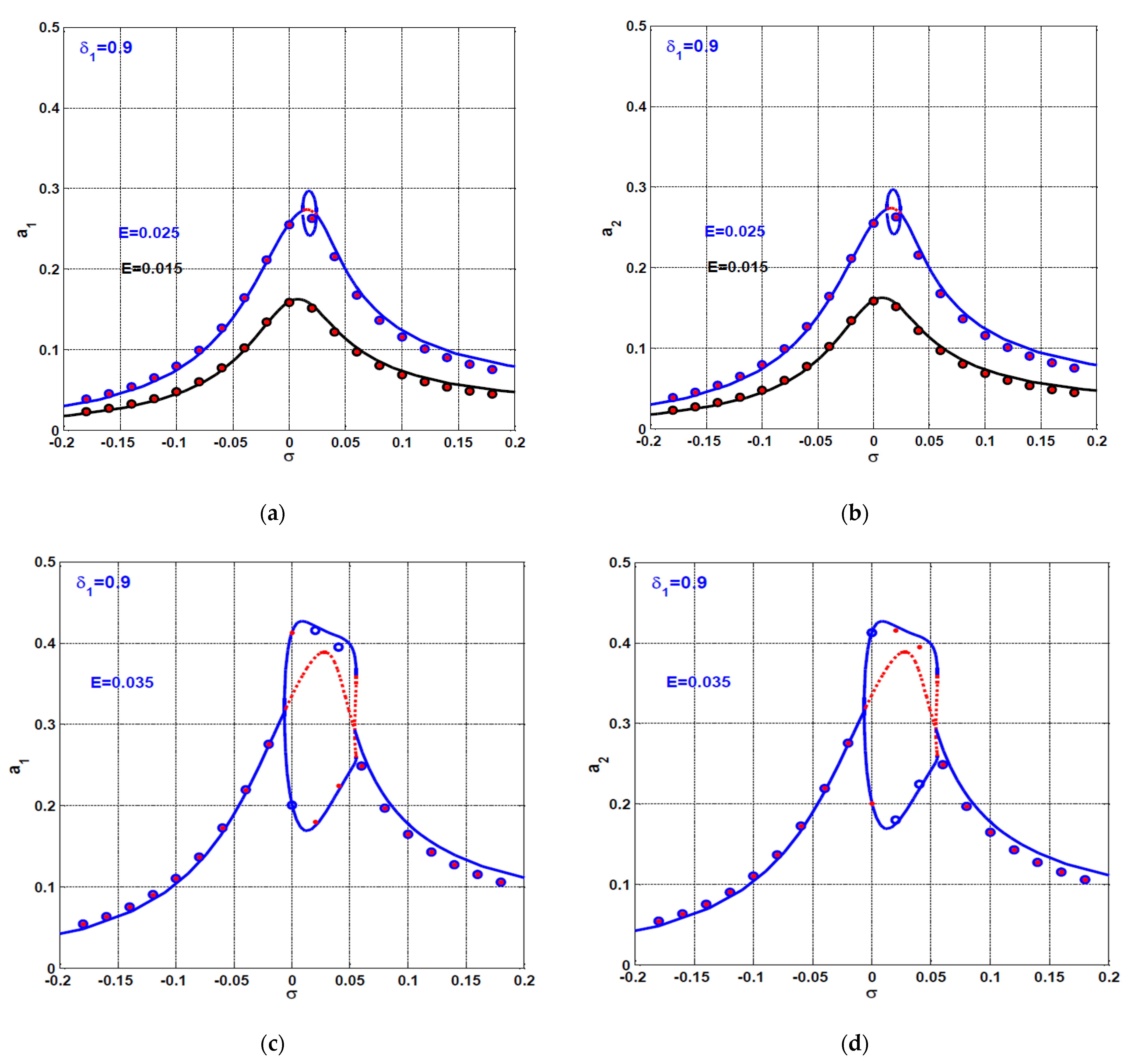
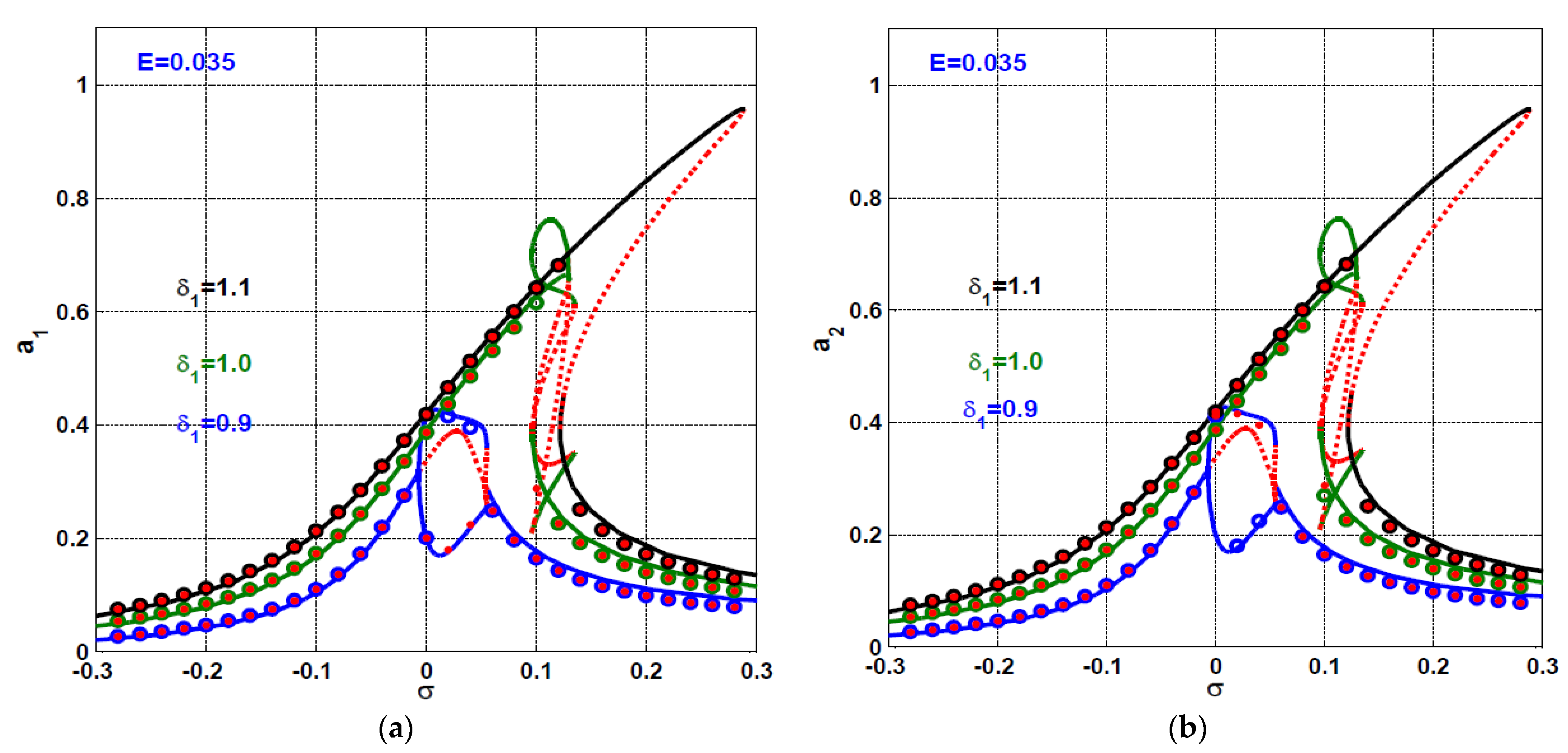
4.1. The Rotor System Response Curves at Small Proportional Gain (${\delta }_1=0.9$)

Figure 2 shows the considered system oscillation amplitudes $a_1$ and $a_2$ against the detuning parameter $\sigma$ via solving Equations (44)–(47) at ${\delta }_1=0.9, E=0.015, 0.025,$ and $0.035$. It is clear from the figure that the system responds as a linear system for the small disc eccentricities (i.e., $E=0.015$), while the nonlinearities dominate the system response as the disc eccentricity increases (i.e., $E=0.025, 0.035$). The figure also shows that at $E=0.025, 0.035$, the system has a bistable solution close to $\sigma =0$, indicating that the rotor system can oscillate harmonically with one of two stable amplitudes depending on the initial conditions. Furthermore, the maximum oscillation amplitude either in the horizontal or the vertical directions is lower than unity (i.e., $a_1<1$ and $a_2<1$) along the $\sigma$ axis, which causes the lateral oscillations for the rotor system without rub and/or impact between the rotor and stator.

Figure 3 shows numerical simulations for the system equations of motion (i.e., Equations (23) and (24)) corresponding to Figure 2c,d when $\sigma =0.0$. The figure shows the system temporal oscillations $u\left(\tau \right)$ and $v\left(\tau \right)$ (i.e., Figure 3a,b) and the corresponding whirling orbits (i.e., Figure 3c) when $E=0.035,{\delta }_1=0.9, {\delta }_2=0.008 \sigma =0, \lambda =5.0$ and ${\mu }_f=0.2$ at the two initial conditions $u\left(0\right)=v\left(0\right)=\dot{u}\left(0\right)=\dot{v}\left(0\right)=0.0$ and $u\left(0\right)=v\left(0\right)=\dot{u}\left(0\right)=\dot{v}\left(0\right)=0.5$. The system’s sensitivity to the initial conditions is shown in Figure 3, where the system performs one of two spinning motions depending on the initial conditions. By examining Figure 3, we can conclude that the rotor system can oscillate by the oscillation amplitudes $a_1=0.42 \& a_2=0.2$ or $a_1=0.2 \& a_2=0.42$ depending on the initial conditions, which agree with Figure 2c,d at $\sigma =0.0$. Accordingly, it is worth mentioning that the obtained nonlinear algebraic system (i.e., Equations (44)–(47)) describes with excellent accuracy the steady-state oscillation amplitude of the studied system (i.e., Equations (23) and (24)) when $\lambda =0.0$.

To investigate the oscillatory behaviors of the rotating disc when the rub-impact force occurs (i.e., when $a_1\ge 1$ and $a_2\ge 1$), the eccentricity response curve and the corresponding bifurcation diagrams are plotted as shown in Figure 4 when $\sigma =0.0$. Utilizing Equations (44)–(47), the system eccentricity response curves are obtained as in Figure 4a,b when $\sigma =0.0, {\delta }_1=0.9$. Figure 4a,b shows that the rotor system can vibrate with oscillation amplitudes lower than unity (i.e., $a_1<1$ and $a_2<1$) if the disc eccentricity $E<0.1176$, which means that the rotating disc can oscillate harmonically without rub and/or impact forces as long as $E<0.1176$. However, when increasing the disc eccentricity to become $0.1176<E<0.4$, the rotor system will perform at an oscillation amplitude higher than unity either in the horizontal or the vertical direction depending on the initial conditions (i.e., $a_1>1$ or $a_2>1$), resulting in rub and/or impact forces between the rotating disc and the pole legs. Moreover, Figure 4a,b illustrates that increasing the disc eccentricity beyond $0.4$ (i.e., $E>0.4$) results in losing the stability of the rotor system.

According to Figure 4a,b, the bifurcation diagram of the system is obtained as shown in Figure 4c utilizing the disc eccentricity as the bifurcation parameter when ${\delta }_1=0.9, \sigma =0, \lambda =5.0, {\mu }_f=0.2$. Figure 4c is obtained by plotting the Poincare map of the instantaneous radial displacement $r\left(\tau \right)=\sqrt{u^2\left(\tau \right)+v^2\left(\tau \right)}$ versus the disc eccentricity via solving of the system original equations (i.e., Equations (23) and (24)) numerically. It is clear from Figure 4c that the rotor system exhibits a periodic solution regardless of the disc eccentricity magnitudes. However, Figure 4a,b show that the system’s stability may be lost when $E>0.4$. Accordingly, we can deduce that the existence of rub and/or impact forces may result in stabilizing the system’s unstable motions. The instantaneous radial displacement $r\left(\tau \right)$ and the corresponding whirling orbit, Poincare map, and frequency spectrum of the rotor system are shown in Figure 5 and Figure 6 according to the obtained results in Figure 4. The radial oscillation $r\left(\tau \right)$ and the corresponding whirling motion of the rotor system are simulated in Figure 5 at $E=0.2$ and ${\mu }_f=0.2$ when the impact stiffness coefficient $\lambda =0.0, 5.0$. Figure 5a–c shows the system temporal oscillation when $\lambda =0$ (i.e., when the rub-impact force is zero), while Figure 5d–f illustrates the system temporal oscillation when $\lambda =5.0$. Generally, Figure 5 confirms that the rotor AMBS system can execute periodic-1 motion either when $\lambda =0.0$ or $\lambda =5.0$ at $E=0.2$. However, the existence of the rub-impact force (i.e., $\lambda =5.0$) between the rotor and stator can play an important role in mitigating the system oscillations (i.e., compare Figure 5b,e).

Figure 6 is a repetition for Figure 5 when the disc eccentricity $E=0.45$. Figure 6a–c shows the system temporal oscillations, whirling motion, and frequency spectrum when $\lambda =0.0$, while Figure 6d–f illustrates the system temporal oscillations, whirling motion, and frequency spectrum when $\lambda =5.0$. It is clear from Figure 6c that the rotor system can perform chaotic oscillations at $E=0.45$ when $\lambda =0.0$, which agrees with Figure 4a,b. However, Figure 6f shows that the existence of rub-impact forces between the rotor and stator (i.e.,$\lambda =5.0$) can force the chaotic oscillation to become a periodic-1, which agrees with the bifurcation diagram given in Figure 4c.

The eccentricity response curve when $\sigma =0.1$ and ${\delta }_1=0.9$ and the corresponding bifurcation diagram are depicted in Figure 7. The steady-state oscillation amplitudes ($a_1$ and $a_2$) are plotted versus the disc eccentricity $E$ via solving Equations (44)–(47) numerically in terms of $E$ as shown in Figure 7a,b, while the bifurcation diagram in Figure 7c is obtained via solving Equations (23) and (24) numerically and plotting the corresponding Poincare map versus the disc eccentricity $E$ when $\sigma =0.1,{\delta }_1=0.9, {\mu }_f=0.2$ and $\lambda =5.0$. Figure 7a,b illustrates that the system can oscillate harmonically without rub-impact occurrences if the disc eccentricity $E<0.116$ while increasing the disc eccentricity beyond $0.116$ (i.e., $E>0.116$) results in losing the stability of the rotor system. Figure 7c confirms that the rotor system can exhibit periodic motions if $E<0.116$, but increasing the disc eccentricity beyond $0.116$ results in periodic-n motion. According to Figure 7c, we can confirm that the existence of the rub-impact force between the rotor and stator may result in stabilizing the unstable oscillations of the rotor system.

The temporal vibrations of the rotor system when $E=0.2, 0.4$ according to Figure 7 are simulated in Figure 8 and Figure 9. Figure 8 simulates the radial oscillation, whirling orbit, and frequency spectrum of the AMBS system at $E=0.2$ when $\lambda =0.0$(as shown in Figure 8a,c), and when $\lambda =5.0$(as shown in Figure 8d–f). It is clear from Figure 8 that the quasiperiodic motion of the system that occurs when $\lambda =0.0$ becomes a periodic one if the rub-impact force is considered (i.e., when $\lambda =5.0$). Furthermore, Figure 9 shows the rotor system temporal oscillations at $E=0.4$ when $\lambda =0.0, 5.0$, where Figure 9a–c shows that the rotor system can respond with chaotic oscillation when the rub and impact forces between the rotor and stator are zero. However, Figure 9d–f confirms that the existence of rub and/or impact forces between the rotor and the pole legs (i.e., $\lambda =5.0$) can force the chaotic motions to become a periodic-13 one.

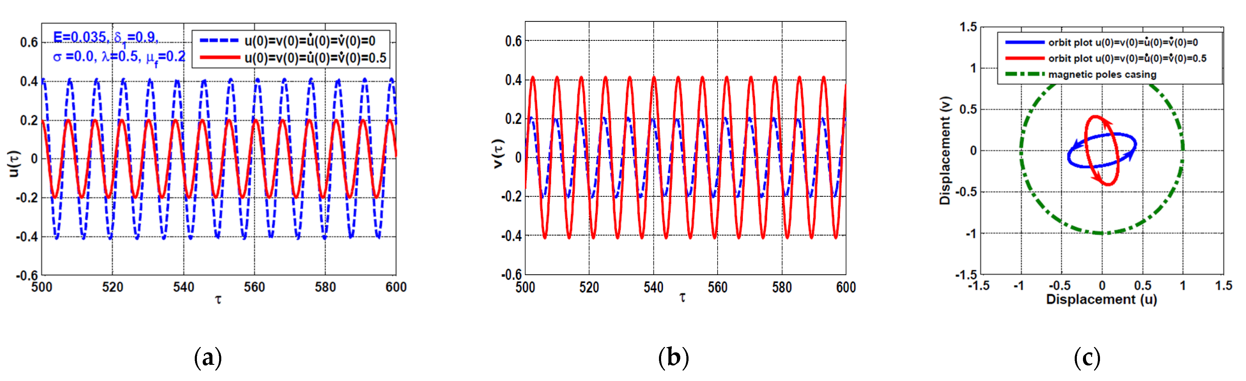
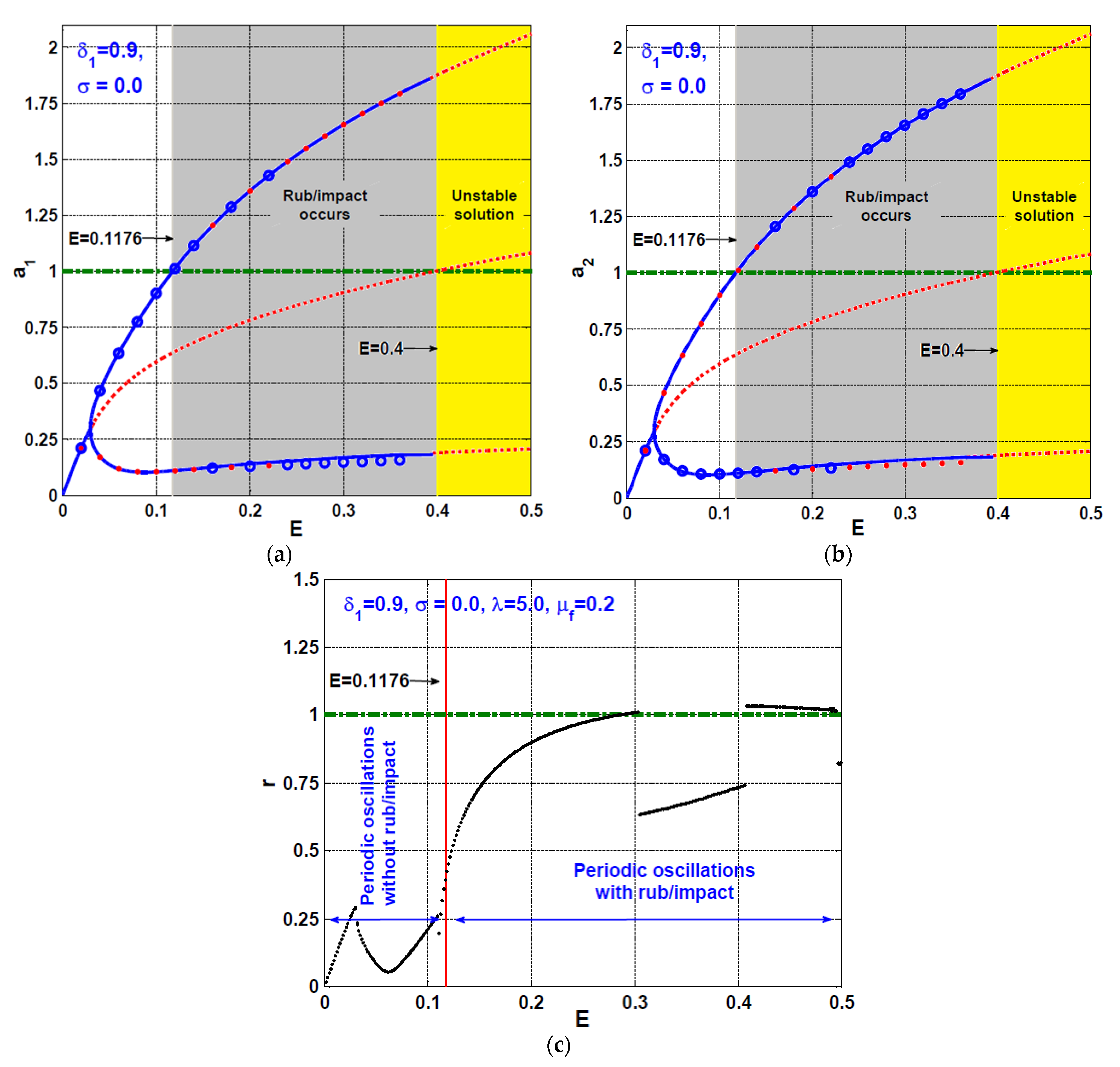
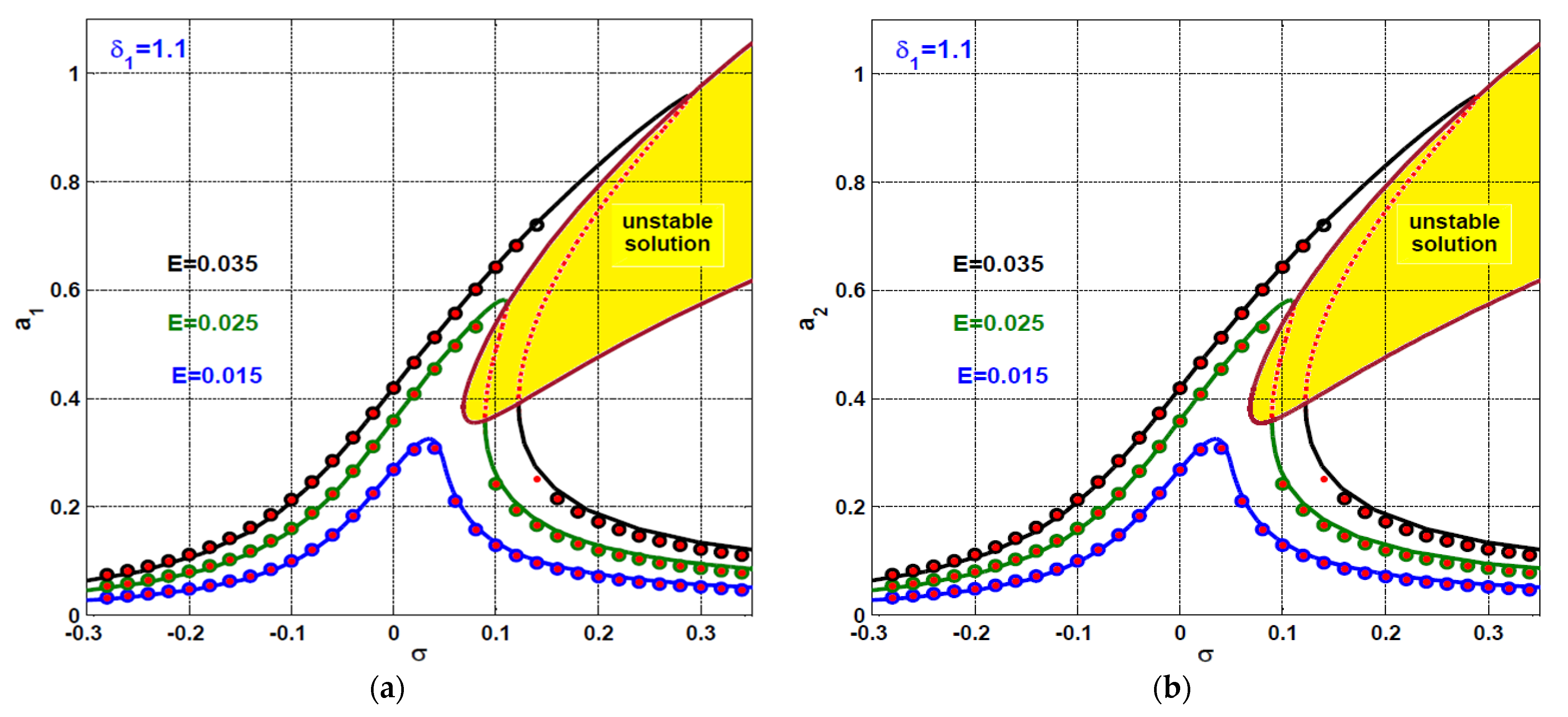
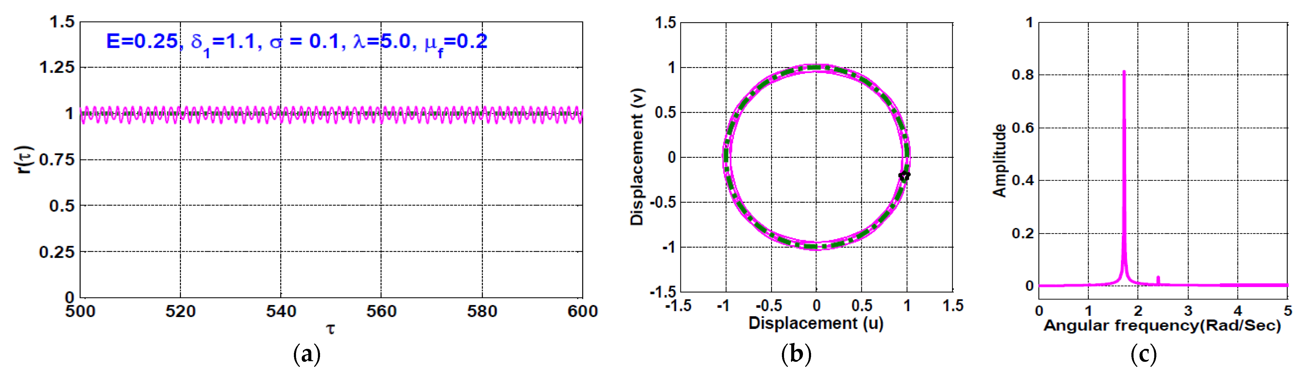
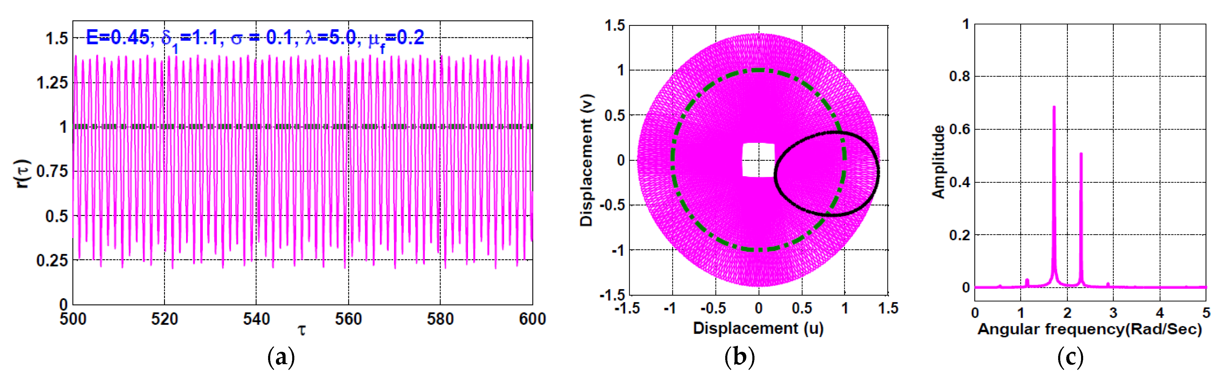
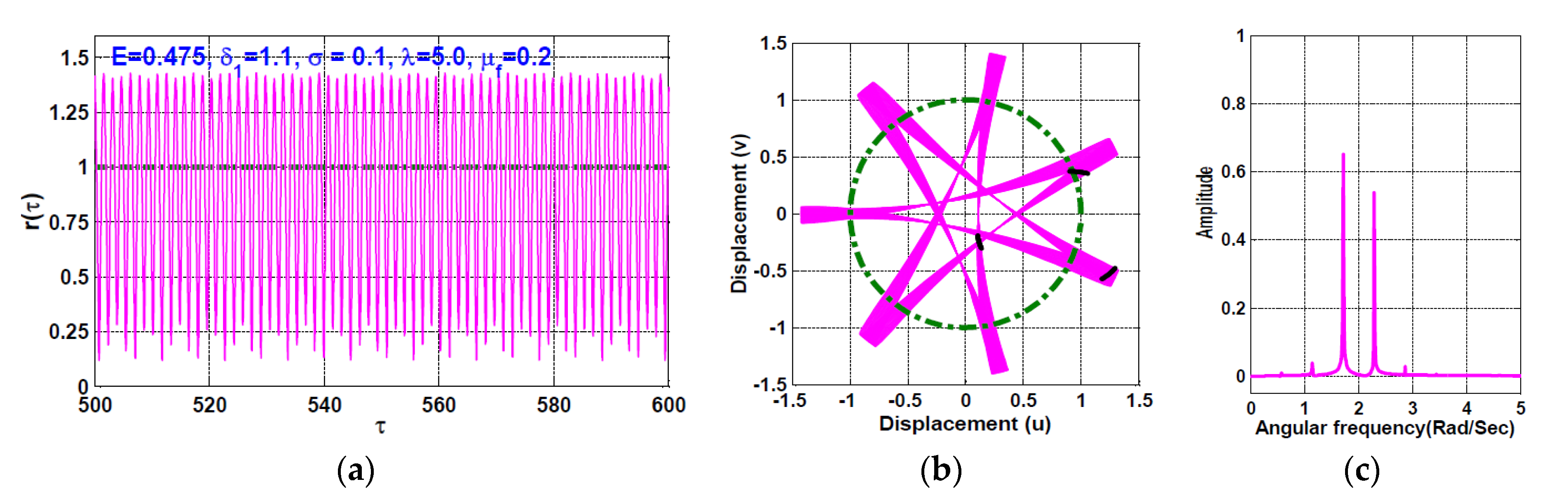
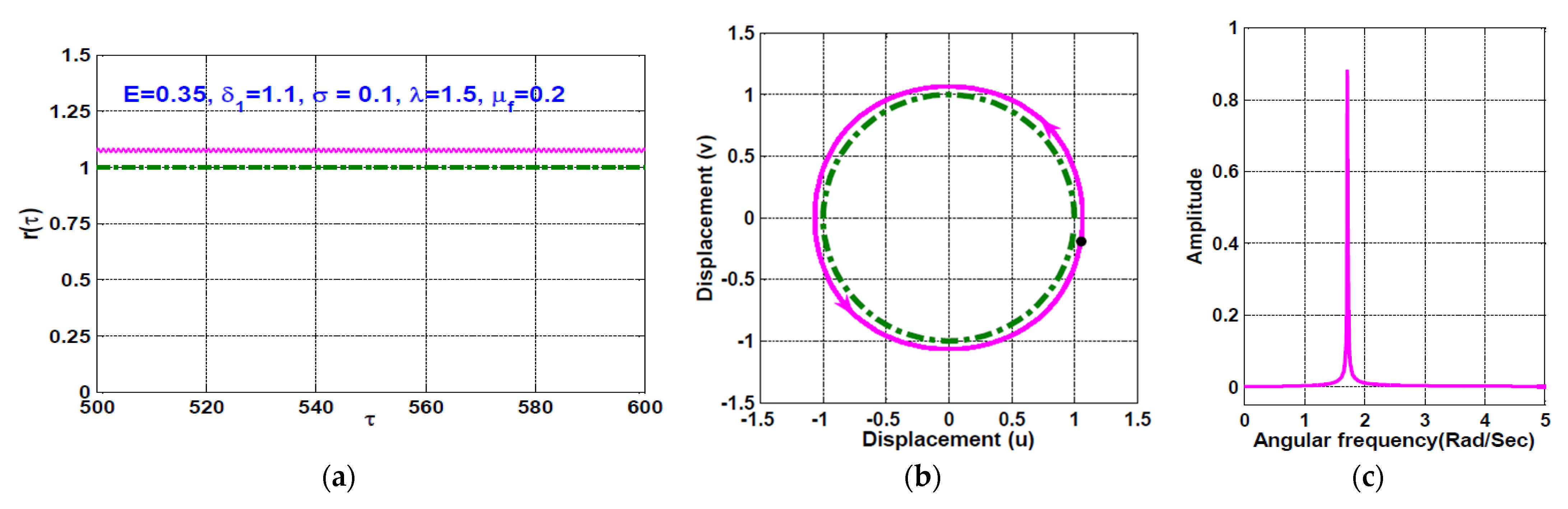
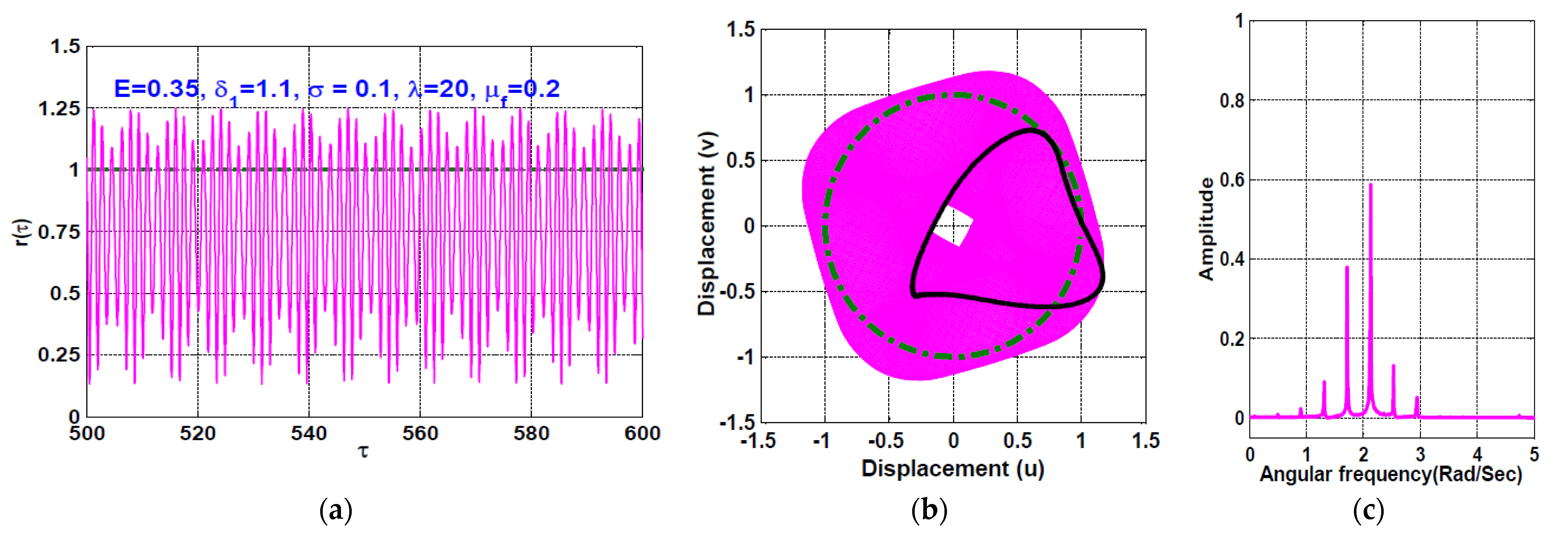
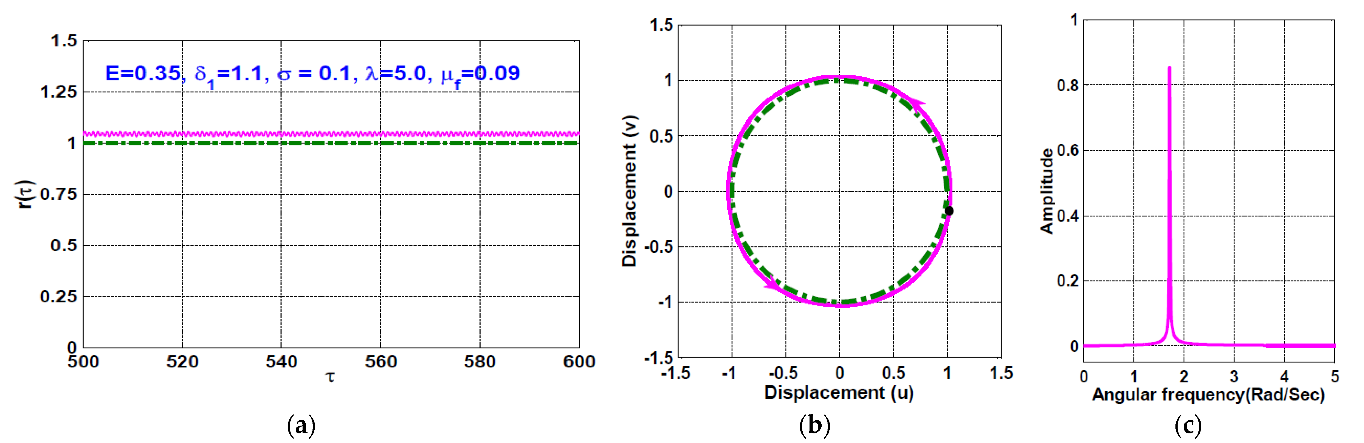
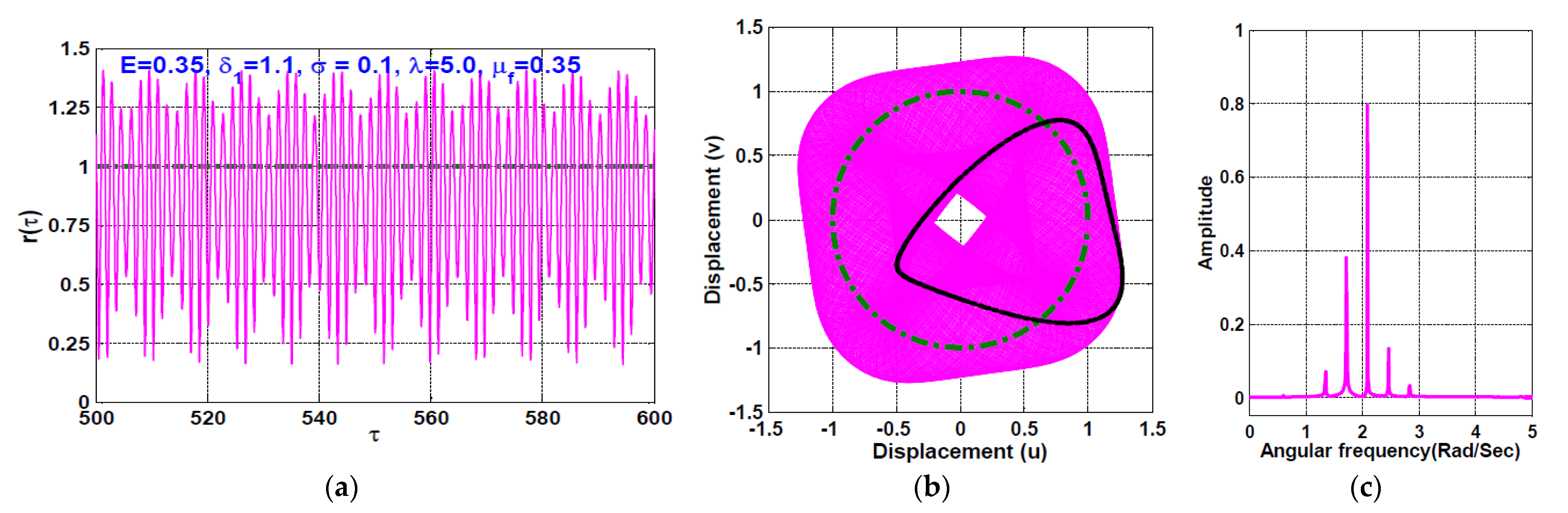
4.2. The Rotor System Response Curves at Large Proportional Gain (${\delta }_1=1.1$)

Figure 10 shows the rotor system response curve at different values of the proportional gain (i.e., ${\delta }_1=0.9, 1.0, 1.1$) when the disc eccentricity $E=0.035$. It is clear from the figure that the increase of the proportional gain increases the rotor oscillation amplitudes and bends the response curves to the right leading to hard spring characteristics. However, in all previously studied control configurations (see Refs. [2,3,9,10,15,16,17]), it is found that the increase of the proportional gain results in increasing the oscillation amplitudes of the rotor system and bends the response curves to the left leading to softening spring characteristics. In addition, Figure 10 depicts that the controlled rotor AMBS can respond as in the case of the cartesian control configuration when the proportional control gain is small (i.e., when ${\delta }_1=0.9$), but increasing the proportional gain to ${\delta }_1=1.1$ causes the response curve to be like that of the radial control configuration (see Refs. [15,17]). Accordingly, we can confirm that the proposed control method behaves like the Cartesian controller when ${\delta }_1=0.9$, but when ${\delta }_1=1.1$, the suggested control algorithm behaves as in the case of radial control configuration. According to Figure 10, the effect of increasing the disc eccentricity on the rotor system spinning speed response curves is illustrated in Figure 11 when ${\delta }_1=1.1$. It is clear from the figure that the system oscillation amplitude is a monotonic increasing function of the disc eccentricity. Moreover, the rotor system responds as a linear system when $E=0.015$, but the nonlinearity dominates the system response when increasing the eccentricity to $E=0.025, 0.035$.

Comparing Figure 2 with Figure 11, we can deduce that the proportional control gain plays an important role in controlling the system dynamical behaviors, where at the low value of ${\delta }_1$, the rotor system exhibits a bistable solution and responds with the maximum oscillation amplitude close to $\sigma =0.0$. However, Figure 11 illustrates that the increase of the proportional gain to ${\delta }_1=1.1$ has bent the frequency response curves to the right leading to hard spring characteristics and a bistable solution on the right-hand side of $\sigma =0.0.$ In addition, the controlled rotor system responds as in the case of the cartesian control configuration (see Refs. [15,17]) as in Figure 2 when ${\delta }_1=0.9$, while the system responds as in the case of radial control strategy (see Refs. [15,17]) as in Figure 11 when ${\delta }_1=1.1$.

According to Figure 11, the eccentricity response curve of the rotor system at ${\delta }_1=1.1$ when $\sigma =0.0$ is illustrated in Figure 12a via solving Equations (44)–(47). It is clear from the figure that the rotor system can oscillate with vibration amplitudes lower than unity (i.e., $a_1<1$ and $a_2<1$) as long as the disc eccentricity $E<0.3888$, which means that the rotating disc can oscillate harmonically without a rub-impact force if $E<0.3888$. However, increasing the disc eccentricity to become $E>0.3888$, the rotor system will perform at an oscillation amplitude higher than unity in both the horizontal and the vertical direction, resulting in rub and/or impact forces among the rotor and the stator. Depending on the reported results in Figure 12a, the system bifurcation diagram is obtained via plotting the steady-state Poincare map for the system original equations (i.e., Equations (23) and (24)) versus the disc eccentricity $E$ when ${\delta }_1=1.1, \sigma =0.0, \lambda =5.0,{\mu }_f=0.2$ as shown in Figure 12b. The figure confirms that the rotor system can execute periodic-1 motions if the eccentricity $E<0.3888$, but for $E>0.3888$, the system performs quasiperiodic oscillations. Comparing Figure 12a,b, we can deduce that the rotor AMBS system executes periodic oscillation as long as the rub-impact force between the rotor and stator does not occur, while the occurrence of a rub-impact force at large disc eccentricities (i.e., $E>0.3888$) results in a quasiperiodic oscillation.

The temporal oscillation of the rotor system according to Figure 12 (i.e., when ${\delta }_1=1.1, \sigma =0.0$) is simulated when the disc eccentricity $E=0.3, 0.45$ as shown in Figure 13 and Figure 14, respectively. the figures are obtained via solving Equations (23) and (24) numerically when $\lambda =5.0, {\mu }_f=0.2$. It is clear from Figure 13 that the system performs periodic-1 motion with oscillation amplitudes lower than unity, where the rub-impact does not occur as is clear in Figure 13b. On the other hand, Figure 14 illustrates the rotor system temporal oscillations according to Figure 12 at $E=0.45$. The figure confirms that the system oscillates with oscillation amplitudes higher than unity, resulting in rub-impact force between the rotor and the pole legs, which ultimately leads to quasiperiodic motion.

Figure 15 is a repetition pf Figure 12, but when the detuning parameter $\sigma =0.1$ (i.e., when $\mathsf{\Omega }=\omega +0.1$). comparing Figure 15 with Figure 12, we can confirm the dominance of the nonlinearity on the system eccentricity response curve, where the system has a bistable solution for some values of the disc eccentricity. In addition, Figure 15a illustrates that the rotor AMBS may encounter rub and/or impact forces if the disc eccentricity $E>0.2371$, which leads to quasiperiodic oscillation as illustrated in Figure 15b. According to Figure 15, numerical simulations for radial oscillation of the rotor system are illustrated in Figure 16, Figure 17 and Figure 18 when $E=0.25, 0.45,$ and $0.475$, respectively. Comparing Figure 16, Figure 17 and Figure 18 with Figure 15, we can demonstrate the great agreement between the analytic results (i.e., Figure 15) and the numerical simulations (i.e., Figure 16, Figure 17 and Figure 18).

The dynamical behavior of the rotor system when ${\delta }_1=1.1$ and $\sigma =0.1$ at different values of both the impact stiffness coefficient ($\lambda$) and the dynamic friction coefficient (${\mu }_f$) is investigated in Figure 19 via plotting the system bifurcation diagrams utilizing $\lambda$ or ${\mu }_f$ as a bifurcation control parameter. Figure 19a shows the qualitative change of the rotor motion with varying the impact stiffness coefficient from $\lambda =1$ to $\lambda =20$ when $E=0.35, {\delta }_1=1.1, \sigma =0.1$ and ${\mu }_f=0.2$, while Figure 19b illustrates the qualitative change of the system motion when varying the dynamic friction coefficient from ${\mu }_f=0.05$ to ${\mu }_f=0.4$ when $E=0.35, {\delta }_1=1.1, \sigma =0.1$ and $\lambda =5.0$. It is clear from Figure 19a that the rotor system executes full annular rub mode with a periodic-1 motion as long as $\lambda <2$, while increasing the impact stiffness coefficient beyond $2$ results in a quasiperiodic partial rub motion. On the other hand, Figure 19b shows that the rotating disc can oscillate with full annular rub mode if ${\mu }_f<0.095$, while increasing the friction coefficient beyond $0.095$ results in a quasiperiodic partial rub motion.

The temporal oscillations of the rotor system according to Figure 19 are simulated as shown in Figure 20, Figure 21, Figure 22 and Figure 23, where Figure 20 and Figure 21 simulate the rotating disc according to Figure 19a when $\lambda =1.5$ and $\lambda =20$, respectively. It is clear from Figure 20 that the rotating disc executes periodic-1 motion with a full annular rub, while the impact force between the rotor and stator disappeared when $\lambda =1.5$. However, Figure 21 shows that the rotor system can perform quasiperiodic oscillation with partial rub mode. Figure 22 and Figure 23 illustrate the temporal oscillations of the rotor system according to Figure 19b when ${\mu }_f=0.09$ and ${\mu }_f=0.35$, respectively. Figure 22 demonstrates that the system may exhibit periodic-1 motion with a full annular rub at ${\mu }_f=0.09$, while the system performs quasiperiodic motion when increasing the friction coefficient to ${\mu }_f=0.35$ as shown in Figure 23.

5. Conclusions

A new control scheme for the 8-pole rotor active magnetic bearing system is introduced for the first time within this article. The system mathematical model is derived including the rub and impact forces between the rotating disc and the 8-pole legs by means of classical mechanics. Including the rub and impact forces between the rotating disc and the poles legs results in obtaining a discontinuous two-degree-of-freedom dynamical system. Accordingly, the derived mathematical model is investigated analytically to determine the conditions at which the system may encounter rub and/or impact forces between the rotor and stator utilizing perturbation methods. Then, the different bifurcation diagrams are plotted to explore the nature of the system motion, either periodic, periodic-n, quasiperiodic, or chaotic. Finally, numerical confirmations for all obtained analytical results are introduced. According to the above discussion, the following remarks can be concluded:

• The proposed control method can behave either as a cartesian control strategy or as radial control one depending on the magnitude of the proportional gain.
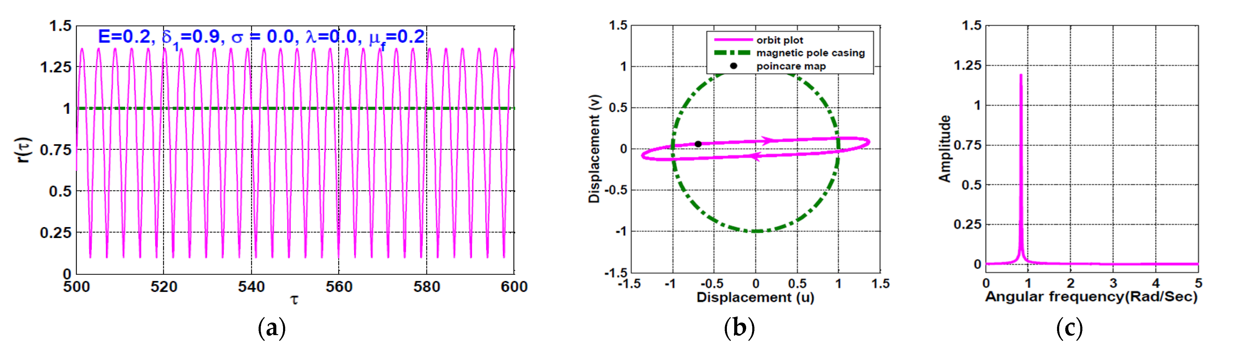
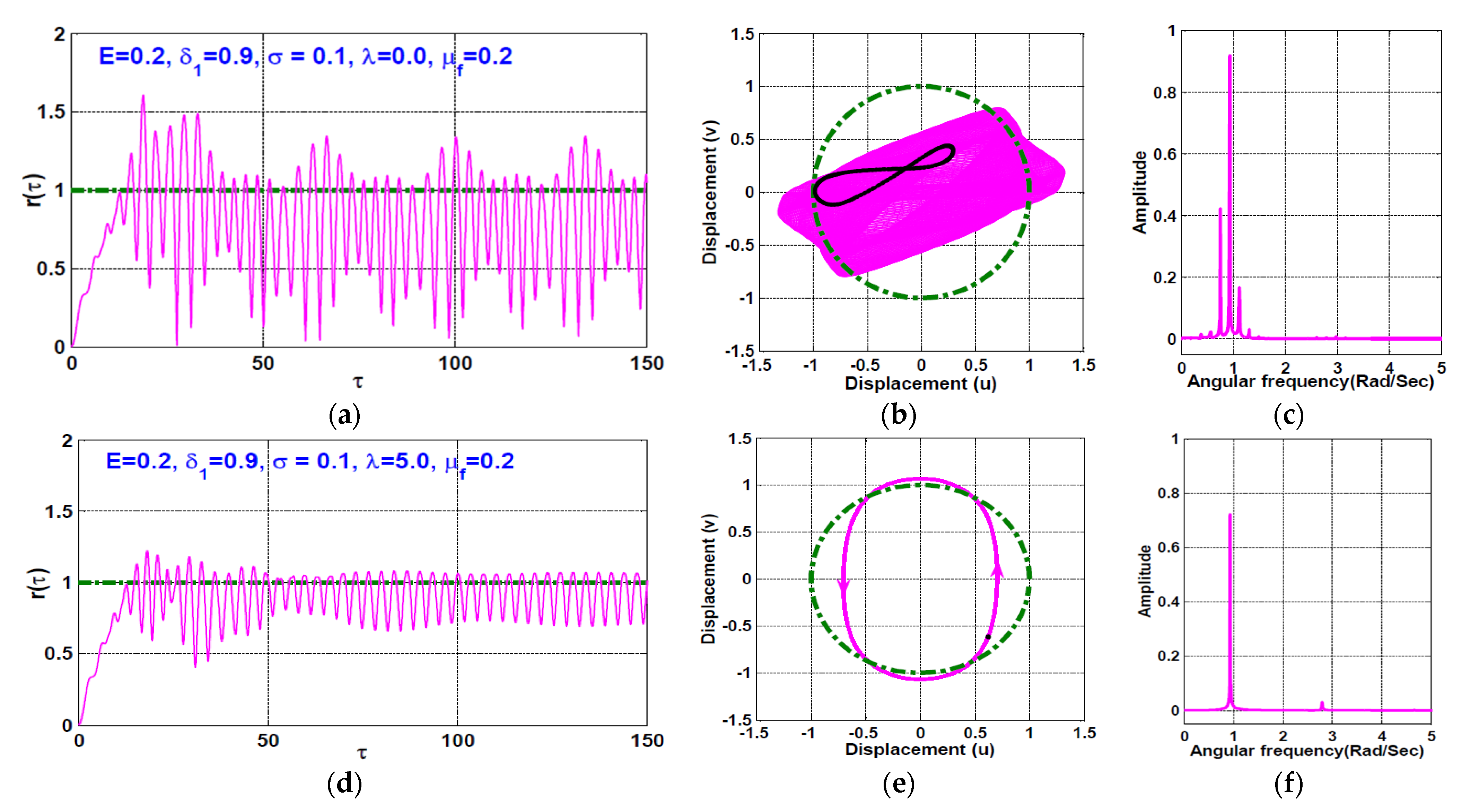
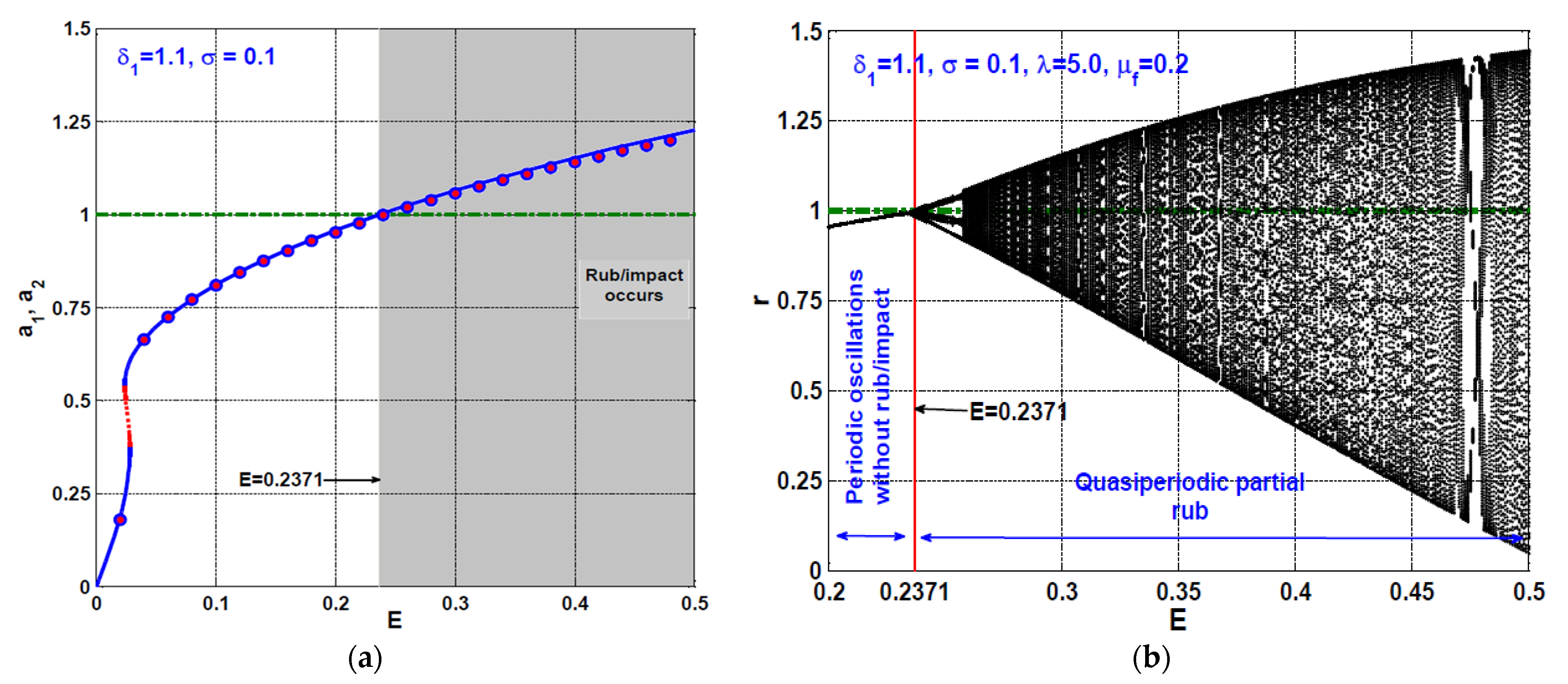
• At small values of the proportional gain (i.e., when $0.8<{\delta }_1<1$), the rotor system may exhibit unstable periodic oscillation at the larger disc eccentricities when the impact stiffness coefficient is zero (i.e., when $\lambda =0.0$).
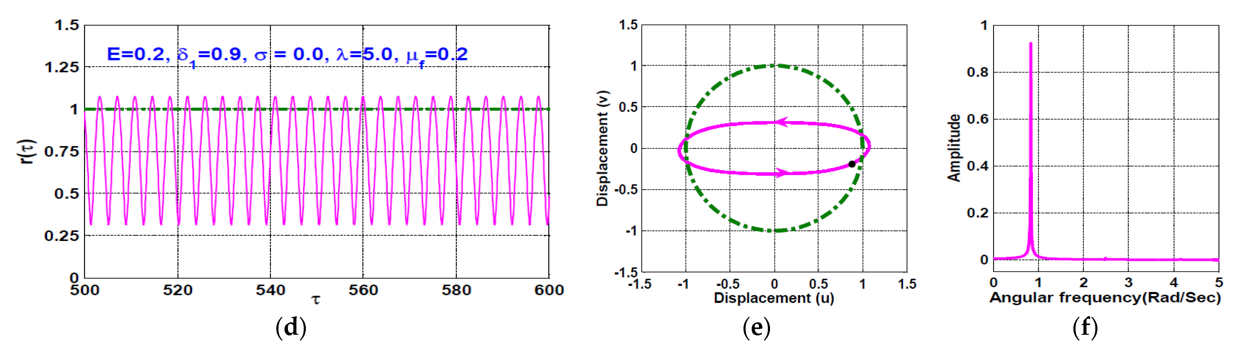
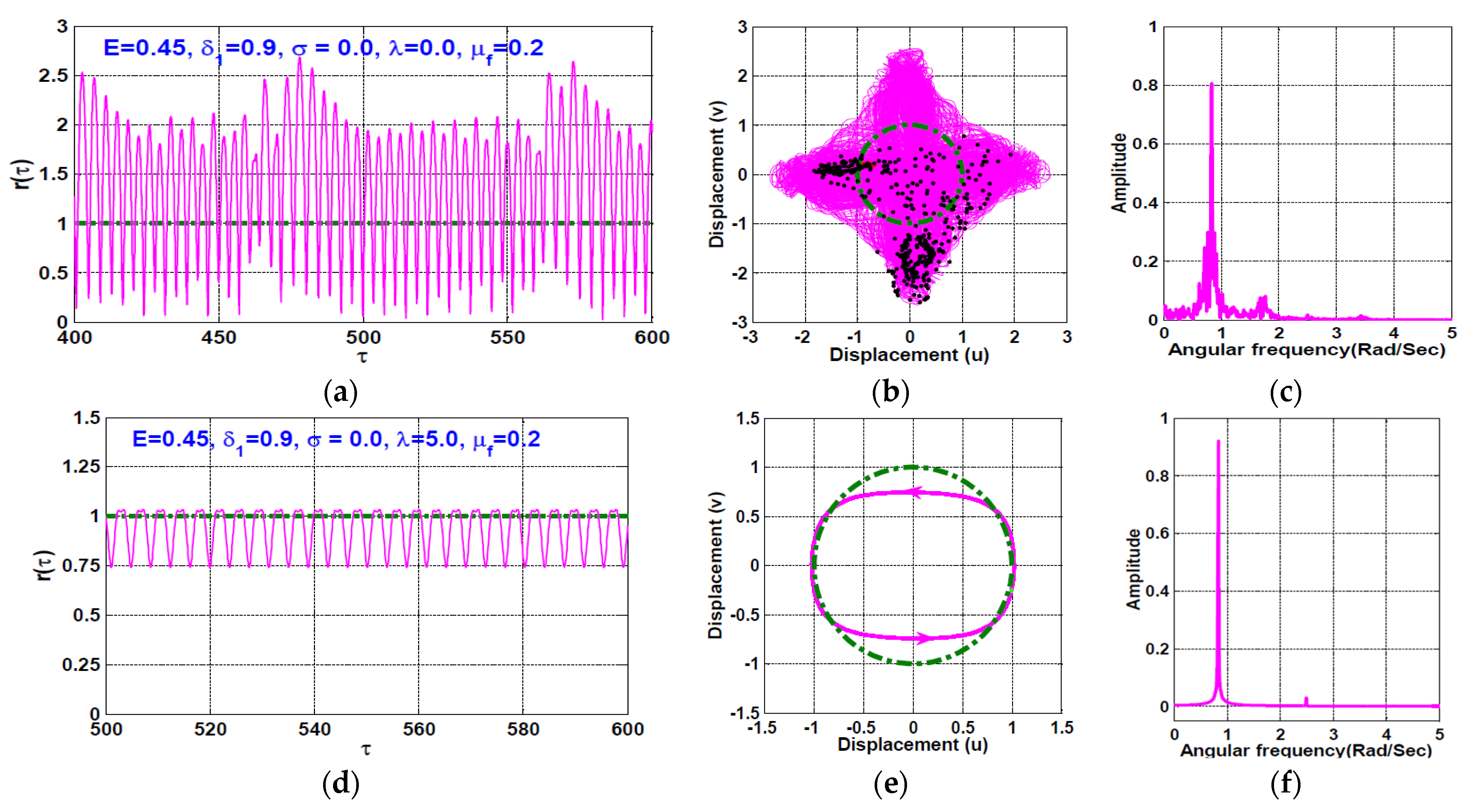
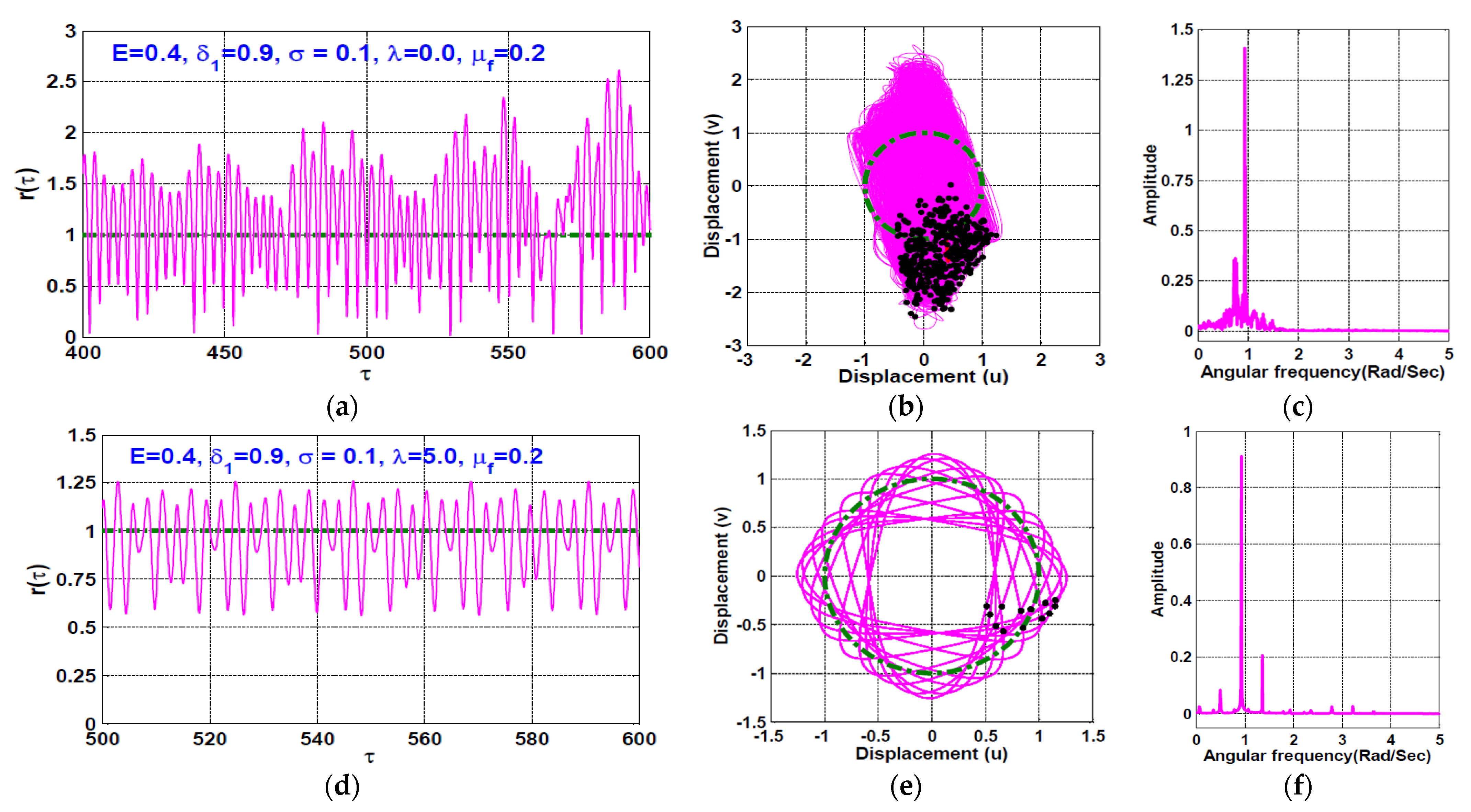
• At large disc eccentricities, the existence of rub and/or impact forces between the rotating disc and the poles legs can cause the chaotic and quasiperiodic motions of the rotor system to become periodic-n motions.
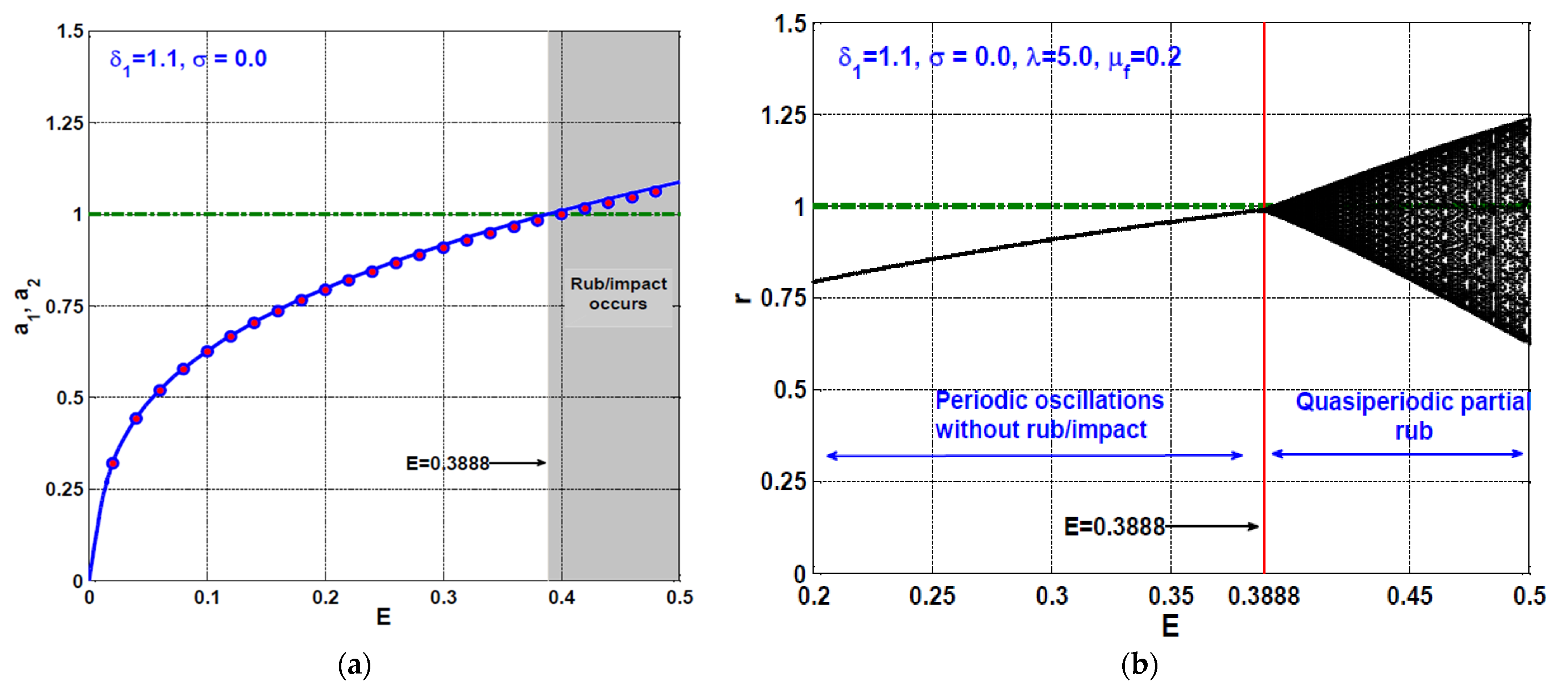
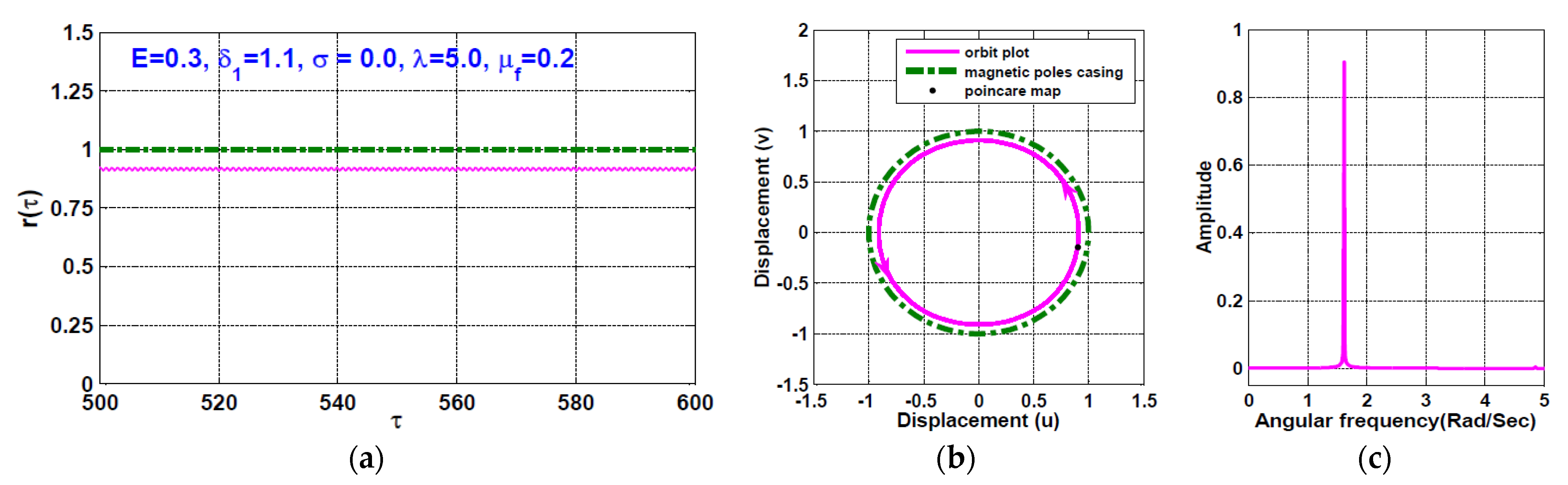
• The rotor system exhibits stable periodic motions at large values of the proportional gain (i.e., when ${\delta }_1>1.1$) as long as the rub-impact force between the rotor and stator does not occur regardless of the disc eccentricity magnitude.
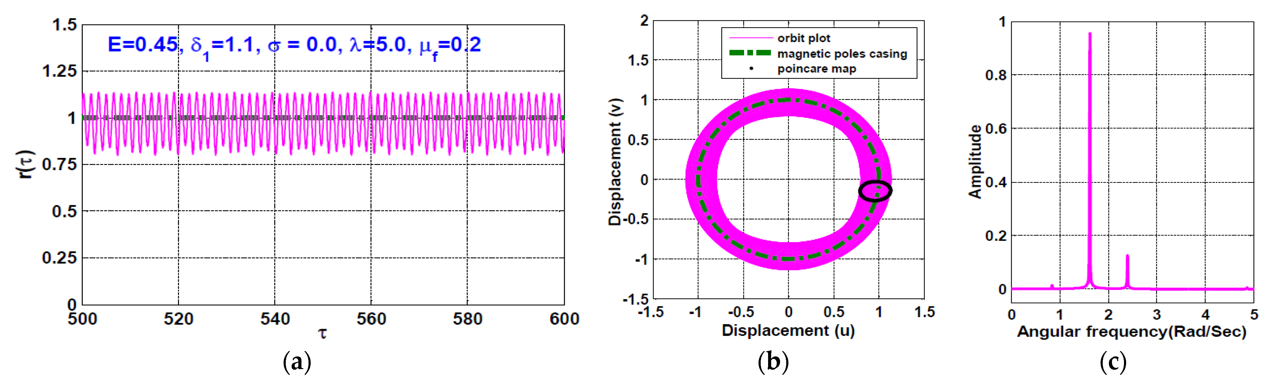
• The occurrence of rub and/or impact forces between the rotor and stator (when ${\delta }_1>1.1$) results in a quasiperiodic oscillation for the rotor system.
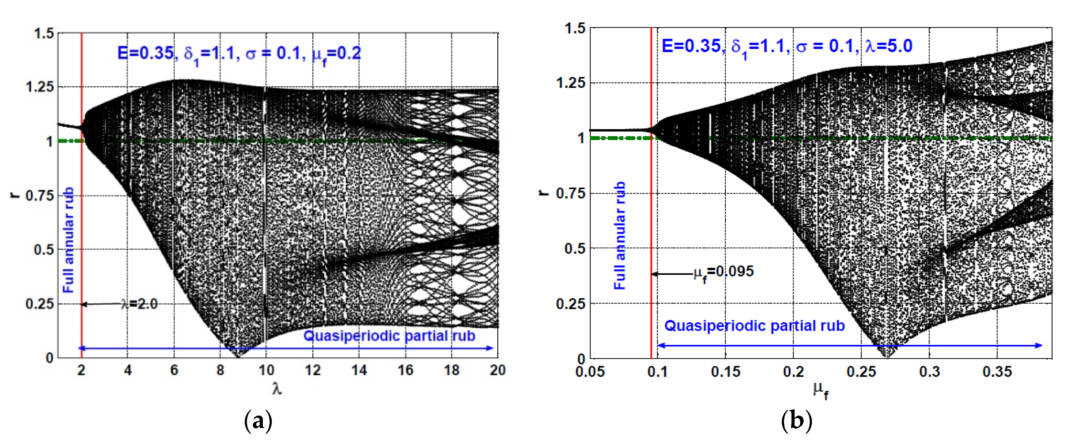
• The magnitudes of both the impact stiffness coefficient ($\lambda$) and the friction coefficient $({\mu }_f$) have a great influence on the rotor oscillation mode, where the system can oscillate in full annular rub mode or a quasiperiodic partial rub mode depending on the magnitudes of the impact stiffness coefficient and the dynamic friction coefficient.

References

1. Ji, J.C.; Yu, L.; Leung, A.Y.T. Bifurcation behavior of a rotor supported by active magnetic bearings. J. Sound Vib. 2000, 235, 133–151. [Google Scholar] [CrossRef]
2. Saeed, N.A.; Eissa, M.; El-Ganini, W.A. Nonlinear oscillations of rotor active magnetic bearings system. Nonlinear Dyn. 2013, 74, 1–20. [Google Scholar] [CrossRef]
3. Ji, J.C.; Hansen, C.H. Non-linear oscillations of a rotor in active magnetic bearings. J. Sound Vib. 2001, 240, 599–612. [Google Scholar] [CrossRef]
4. Ji, J.C.; Leung, A.Y.T. Non-linear oscillations of a rotor-magnetic bearing system under superharmonic resonance conditions. Int. J. Nonlinear. Mech. 2003, 38, 829–835. [Google Scholar] [CrossRef]
5. Yang, X.D.; An, H.Z.; Qian, Y.J.; Zhang, W.; Yao, M.H. Elliptic Motions and Control of Rotors Suspending in Active Magnetic Bearings. J. Comput. Nonlinear Dyn. 2016, 11, 054503. [Google Scholar] [CrossRef]
6. Zhang, W.; Zhan, X.P. Periodic and chaotic motions of a rotor-active magnetic bearing with quadratic and cubic terms and time-varying stiffness. Nonlinear Dyn. 2005, 41, 331–359. [Google Scholar] [CrossRef]
7. Zhang, W.; Yao, M.H.; Zhan, X.P. Multi-pulse chaotic motions of a rotor-active magnetic bearing system with time-varying stiffness. Chaos Solitons Fractals 2006, 27, 175–186. [Google Scholar] [CrossRef]
8. Zhang, W.; Zu, J.W.; Wang, F.X. Global bifurcations and chaos for a rotor-active magnetic bearing system with time-varying stiffness. Chaos Solitons Fractals 2008, 35, 586–608. [Google Scholar] [CrossRef]
9. Eissa, M.; Saeed, N.A.; El-Ganini, W.A. Saturation-based active controller for vibration suppression of a four-degree-of-freedom rotor-AMBs. Nonlinear Dyn. 2014, 76, 743–764. [Google Scholar] [CrossRef]
10. Saeed, N.A.; Kandil, A. Lateral vibration control and stabilization of the quasiperiodic oscillations for rotor-active magnetic bearings system. Nonlinear Dyn. 2019, 98, 1191–1218. [Google Scholar] [CrossRef]
11. Wu, R.; Zhang, W.; Yao, M.H. Nonlinear vibration of a rotor-active magnetic bearing system with 16-pole legs. In Proceedings of the International Design Engineering Technical Conferences and Computers and Information in Engineering Conference, Cleveland, OH, USA, 6–9 August 2017. [Google Scholar] [CrossRef]
12. Wu, R.; Zhang, W.; Yao, M.H. Analysis of nonlinear dynamics of a rotor-active magnetic bearing system with 16-pole legs. In Proceedings of the International Design Engineering Technical Conferences and Computers and Information in Engineering Conference, Cleveland, OH, USA, 6–9 August 2017. [Google Scholar] [CrossRef]
13. Wu, R.Q.; Zhang, W.; Yao, M.H. Nonlinear dynamics near resonances of a rotor-active magnetic bearings system with 16-pole legs and time varying stiffness. Mech. Syst. Signal Process. 2018, 100, 113–134. [Google Scholar] [CrossRef]
14. Zhang, W.; Wu, R.Q.; Siriguleng, B. Nonlinear Vibrations of a Rotor-Active Magnetic Bearing System with 16-Pole Legs and Two Degrees of Freedom. Shock. Vib. 2020, 2020, 5282904. [Google Scholar] [CrossRef]
15. Saeed, N.A.; Kandil, A. Two different control strategies for 16-pole rotor active magnetic bearings system with constant stiffness coefficients. Appl. Math. Model. 2021, 92, 1–22. [Google Scholar] [CrossRef]
16. Kandil, A.; Sayed, M.; Saeed, N.A. On the nonlinear dynamics of constant stiffness coefficients 16-pole rotor active magnetic bearings system. Eur. J. Mech. A/Solids 2020, 84, 104051. [Google Scholar] [CrossRef]
17. Saeed, N.A.; Awwad, E.M.; El-Meligy, M.A.; Nasr, E.S.A. Radial Versus Cartesian Control Strategies to Stabilize the Nonlinear Whirling Motion of the Six-Pole Rotor-AMBs. IEEE Access 2020, 8, 138859–138883. [Google Scholar] [CrossRef]
18. Saeed, N.A.; Mahrous, E.; Awrejcewicz, J. Nonlinear dynamics of the six-pole rotor-AMBs under two different control configurations. Nonlinear Dyn. 2020, 101, 2299–2323. [Google Scholar] [CrossRef]
19. Ishida, Y.; Inoue, T. Vibration suppression of nonlinear rotor systems using a dynamic damper. J. Vib. Control. 2007, 13, 1127–1143. [Google Scholar] [CrossRef]
20. Saeed, N.A.; Kamel, M. Nonlinear PD-controller to suppress the nonlinear oscillations of horizontally supported Jeffcott-rotor system. Int. J. Nonlinear Mech. 2016, 87, 109–124. [Google Scholar] [CrossRef]
21. Saeed, N.A.; Kamel, M. Active magnetic bearing-based tuned controller to suppress lateral vibrations of a nonlinear Jeffcott rotor system. Nonlinear Dyn. 2017, 90, 457–478. [Google Scholar] [CrossRef]
22. Saeed, N.A.; El-Ganaini, W.A. Time-delayed control to suppress the nonlinear vibrations of a horizontally suspended Jeffcott-rotor system. Appl. Math. Model. 2017, 44, 523–539. [Google Scholar] [CrossRef]
23. Saeed, N.A. On the steady-state forward and backward whirling motion of asymmetric nonlinear rotor system. Eur. J. Mech. A Solids 2019, 80, 103878. [Google Scholar] [CrossRef]
24. Saeed, N.A. On vibration behavior and motion bifurcation of a nonlinear asymmetric rotating shaft. Arch. Appl. Mech. 2019, 89, 1899–1921. [Google Scholar] [CrossRef]
25. Ishida, Y.; Yamamoto, T. Linear and Nonlinear Rotordynamics: A Modern Treatment with Applications, 2nd ed.; Wiley-VCH Verlag GmbH & Co. KGaA: New York, NY, USA, 2012. [Google Scholar] [CrossRef]
26. Schweitzer, G.; Maslen, E.H. Magnetic Bearings: Theory, Design, and Application to Rotating Machinery; Springer: Berlin/Heidelberg, Germany, 2009. [Google Scholar] [CrossRef]
27. Saeed, N.A.; Awwad, E.M.; El-Meligy, M.A.; Nasr, E.S.A. Analysis of the rub-impact forces between a controlled nonlinear rotating shaft system and the electromagnet pole legs. Appl. Math. Model. 2021, 93, 792–810. [Google Scholar] [CrossRef]
28. Saeed, N.A.; El-Bendary, S.I.; Sayed, M.; Mohamed, M.S.; Elagan, S.K. On the oscillatory behaviours and rub-impact forces of a horizontally supported asymmetric rotor system under position-velocity feedback controller. Lat. Am. J. Solids Struct. 2021, 18. [Google Scholar] [CrossRef]
29. PáezChávez, J.; Hamaneh, V.V.; Wiercigroch, M. Modelling and experimental verification of an asymmetric Jeffcott rotor with radial clearance. J. Sound Vib. 2015, 334, 86–97. [Google Scholar] [CrossRef]
30. Cong, F.; Chen, J.; Dong, G.; Huang, K. Experimental validation of impact energy model for the rub-impact assessment in a rotor system. Mech. Syst. Signal Process. 2011, 25, 2549–2558. [Google Scholar] [CrossRef]
31. Nayfeh, A.H.; Mook, D.T. Nonlinear Oscillations; Wiley: New York, NY, USA, 1995. [Google Scholar] [CrossRef]
Figure 1. (a) 8-pole rotor active magnetic bearing system in its nominal position; (b) 8-pole rotor active magnetic bearing system with rub and impact forces between the rotor and stator.
Symmetry 13 01502 g001
Figure 2. Spinning-speed response curves (i.e., Ω = ω s + σ ) of the rotor AMBS at δ 1 = 0.9 when E = 0.015 ,   0.025 , and 0.035 : (a,c) oscillation amplitude in X direction, (b,d) oscillation amplitude in Y direction.
Symmetry 13 01502 g002
Figure 3. (a,b) The steady-state temporal oscillations, and (c) the corresponding whirling motion of the rotor AMBS according to Figure 2 when σ = 0   (i.e., when Ω = ω s ) at the two initial conditions u ( 0 ) = v ( 0 ) = u ˙ ( 0 ) = v ˙ ( 0 ) = 0.0 and u ( 0 ) = v ( 0 ) = u ˙ ( 0 ) = v ˙ ( 0 ) = 0.5 .
Symmetry 13 01502 g003
Figure 4. (a,b) The eccentricity response curves of the rotor AMBS when δ 1 = 0.9 ,   σ = 0.0 , and (c) the corresponding bifurcation diagram when λ = 5 and μ f = 0.2 .
Symmetry 13 01502 g004
Figure 5. The steady-state radial oscillation r ( τ ) , the whirling orbit, and frequency spectrum of the rotor AMBS according to Figure 4 when E = 0.2 ,   δ 1 = 0.9 ,   σ = 0.0 : (ac) Steady-state radial oscillation r ( τ ) , the whirling orbit, and frequency spectrum when the rub-impact is neglected (i.e., λ = 0.0 ), (df) steady-state radial oscillation r ( τ ) , the whirling orbit, and frequency spectrum when λ = 5.0 , μ f = 0.2 .
Symmetry 13 01502 g005aSymmetry 13 01502 g005b
Figure 6. The steady-state radial oscillation r ( τ ) , the whirling orbit, and frequency spectrum of the rotor AMBS according to Figure 4 when E = 0.45 ,   δ 1 = 0.9 ,   σ = 0.0 : (ac) Steady-state radial oscillation r ( τ ) , the whirling orbit, and frequency spectrum when the rub-impact is neglected (i.e., λ = 0.0 ), (df) steady-state radial oscillation r ( τ ) , the whirling orbit, and frequency spectrum when λ = 5.0 , μ f = 0.2 .
Symmetry 13 01502 g006
Figure 7. (a,b) The eccentricity response curves of the rotor AMBS when δ 1 = 0.9 ,   σ = 0.1 , and (c) the corresponding bifurcation diagram when λ = 5 and μ f = 0.2 .
Symmetry 13 01502 g007
Figure 8. The steady-state radial oscillation r ( τ ) , the whirling orbit, and frequency spectrum of the rotor AMBS according to Figure 7 when E = 0.2 ,   δ 1 = 0.9 ,   σ = 0.1 : (ac) Steady-state radial oscillation r ( τ ) , the whirling orbit, and frequency spectrum when the rub-impact is neglected (i.e., λ = 0.0 ), (df) steady-state radial oscillation r ( τ ) , the whirling orbit, and frequency spectrum when λ = 5.0 , μ f = 0.2 .
Symmetry 13 01502 g008
Figure 9. The steady-state radial oscillation r ( τ ) , the whirling orbit, and frequency spectrum of the rotor AMBS according to Figure 7 when E = 0.4 ,   δ 1 = 0.9 ,   σ = 0.1 : (ac) Steady-state radial oscillation r ( τ ) , the whirling orbit, and frequency spectrum when the rub-impact is neglected (i.e., λ = 0.0 ), (df) steady-state radial oscillation r ( τ ) , the whirling orbit, and frequency spectrum when λ = 5.0 , μ f = 0.2 .
Symmetry 13 01502 g009
Figure 10. Spinning-speed response curves (i.e., Ω = ω s + σ ) of the rotor AMBS at E = 0.035 when δ 1 = 0.9 ,   1.0 , and 1.1 : (a) oscillation amplitude in X direction, (b) oscillation amplitude in Y direction.
Symmetry 13 01502 g010
Figure 11. Spinning-speed response curves (i.e., Ω = ω s + σ ) of the rotor AMBS at δ 1 = 1.1 when E = 0.015 ,   0.025 , and 0.035 : (a) oscillation amplitude in X direction, (b) oscillation amplitude in Y direction.
Symmetry 13 01502 g011
Figure 12. (a) The eccentricity response curves of the rotor AMBS when δ 1 = 1.1 ,   σ = 0.0 , and (b) the corresponding bifurcation diagram when λ = 5 and μ f = 0.2 .
Symmetry 13 01502 g012
Figure 13. (a) The steady-state radial oscillation r ( τ ) , (b) the whirling orbit, and (c) frequency spectrum of the rotor AMBS according to Figure 12 when E = 0.3 ,   δ 1 = 1.1 ,   σ = 0.0   ,   λ = 5.0 , and μ f = 0.2 .
Symmetry 13 01502 g013
Figure 14. (a)The steady-state radial oscillation r ( τ ) , (b) the whirling orbit, and (c) frequency spectrum of the rotor AMBS according to Figure 12 when E = 0.45 ,   δ 1 = 1.1 ,   σ = 0.0 ,   λ = 5.0 , and μ f = 0.2 .
Symmetry 13 01502 g014
Figure 15. (a) The eccentricity response curves of the rotor AMBS when δ 1 = 1.1 ,   σ = 0.1 , and (b) the corresponding bifurcation diagram when λ = 5 and μ f = 0.2 .
Symmetry 13 01502 g015
Figure 16. (a) The steady-state radial oscillation r ( τ ) , (b) the whirling orbit, and (c) frequency spectrum of the rotor AMBS according to Figure 15 when E = 0.25 ,   δ 1 = 1.1 ,   σ = 0.1 ,   λ = 5.0 , and μ f = 0.2 .
Symmetry 13 01502 g016
Figure 17. (a) The steady-state radial oscillation r ( τ ) , (b) the whirling orbit, and (c) frequency spectrum of the rotor AMBS according to Figure 15 when E = 0.45 ,   δ 1 = 1.1 ,   σ = 0.1 ,   λ = 5.0 , and μ f = 0.2 .
Symmetry 13 01502 g017
Figure 18. (a)The steady-state radial oscillation r ( τ ) , (b) the whirling orbit, and (c) frequency spectrum of the rotor AMBS according to Figure 15 when E = 0.475 ,   δ 1 = 1.1 ,   σ = 0.1 ,   λ = 5.0 , and μ f = 0.2 .
Symmetry 13 01502 g018
Figure 19. The rotor system bifurcation diagrams when E = 0.35 ,   δ 1 = 1.1 , and σ = 0.1 : (a) Stiffness coefficient λ versus r when μ f = 0.2 , and (b) friction coefficient μ f versus r when λ = 5.0 .
Symmetry 13 01502 g019
Figure 20. (a) The steady-state radial oscillation r ( τ ) , (b) the whirling orbit, and (c) frequency spectrum of the rotor AMBS according to Figure 19a (i.e., when E = 0.35 ,   δ 1 = 1.1 ,   σ = 0.1 ,   μ f = 0.2 ) at λ = 1.5 .
Symmetry 13 01502 g020
Figure 21. (a) The steady-state radial oscillation r ( τ ) , (b) the whirling orbit, and (c) frequency spectrum of the rotor AMBS according to Figure 19a (i.e., when E = 0.35 ,   δ 1 = 1.1 ,   σ = 0.1 ,   μ f = 0.2 ) at λ = 20 .
Symmetry 13 01502 g021
Figure 22. (a) The steady-state radial oscillation r ( τ ) , (b) the whirling orbit, and (c) frequency spectrum of the rotor AMBS according to Figure 19b (i.e., when E = 0.35 ,   δ 1 = 1.1 ,   σ = 0.1 , λ = 5 ) at μ f = 0.09 .
Symmetry 13 01502 g022
Figure 23. (a) The steady-state radial oscillation r ( τ ) , (b) the whirling orbit, and (c) frequency spectrum of the rotor AMBS according to Figure 19b (i.e., when E = 0.35 ,   δ 1 = 1.1 ,   σ = 0.1 , λ = 5 ) at μ f = 0.35 .
Symmetry 13 01502 g023