Control Theory Application for Swing Up and Stabilisation of Rotating Inverted Pendulum

Abstract

This paper introduces a new scheme for sliding mode control using symmetry principles for a rotating inverted pendulum, with the possibility of extension of this control scheme to other dynamic systems. This was proven for swing up and stabilisation control problems via the new sliding mode control scheme using both simulations and experiments of rotary inverted pendulum (RIP) underactuated systems. According to the Lyapunov theory, a section of the pendulum was compensated with a scale error in the upright position, as the desired trajectory was followed by the pendulum arm section. As the RIP’s dynamic equations were nonlinearly complex and coupled, the complex internal dynamics made the task of controller design difficult. The system control for the pathway of the reference model of the rotational actuator with the application of the sliding mode technique for moving back and forth up the inverted pendulum’s structure, till the arm to reach the linear range round the vertical upright position, was created and tested in an existent device. The stabilisation scheme was switched on in the sliding mode as soon as the arm reached the linear range. A comparison of the stabilisation performance for the same rotating inverted pendulum as discussed by other authors revealed that the proposed controller was more flexible and reliable in terms of the swing up and stabilisation time.

1. Introduction

There are three main components of a rotary inverted pendulum (RIP), namely, link 1 and link 2 of the pendulum, and a motor (Figure 1). The working mechanism of the RIP framework is that link 1 is driven by the motor with the appropriate control order to such an extent that the descending link 2 can be adjusted in the vertical position [1]. It is well known in the domain of a control hypothesis that RIP is one of the most complex control problems [2]. Wiener, Johnson, et al. based their work on humans and other animals to study their movements because some types of machines behave similarly [3]. Humans and animals control their mechanisms based on environmental variables when they are in a reliable terrain while moving or performing certain tasks [3].

The authors in [4] regarding the design of general feedback theory of human behaviour, started with theoretical model before outlining the application of the physical model.

There is another idea that its components map onto the adverse feedback system within the existing models of behaviour for artificial control systems [5]. The movement control of a two-legged robot is based on the inverse pendulum theory [6]. Its good example is an RIP system for nonlinear underactuated mechanical systems to practice the control theory and with special emphasis on robotics for applications [7]. Saleem et al. and Jadlovska et al. provided the mathematical equations and numerous calculations, to find the appropriate way for the nominal trajectory to control the RIP [8]. Wen et al. based their work [9] on the Lyapunov theory control for nonlinear dynamics associated with the RIP in an optimal control effort. In our case, for RIP, we solved this problem by using K_our and an LQR controller; we compared our results with the other authors’ [10,11,12,13,14] because these authors examined the same problem with LQR [5,15]. Some authors [16,17,18,19,20] have tested and implemented the theory of fractional calculus with a PID controller [21]. Irrespective of their prominence, traditional PID controllers come up short on the global asymptotic steadiness verification [21,22]. The contribution of this article is the amalgamation of an upgraded and adjustment control scheme for the RIP system. On a very basic level, the proposed scheme serves simultaneously as the adjuster and the controller. These controllers utilise the state input of the link 1 angle (β), the link 2 angle (α), and their time subordinates to produce the ideal force (or voltage) control orders to upright balance link 2, while continuously turning link 1 as close as is conceivable to its unique position, separately [23,24,25,26]. In this study, we realised the occasion-based procedures to control a rotary pendulum, for both swinging up and balancing out its arm [27]. Swinging up a rotary pendulum is an old and testing issue in the field of nonlinear control research [28,29,30]. The rest of this paper is organised as follows: The RIP dynamics and its state space models are discussed in Section 4, Section 5 and Section 6. The stabilisation and swing up controllers principle is shown in Section 6. Section 7 and Section 8 show the theoretical and experimental results, and finally, in the end, a conclusion is presented.

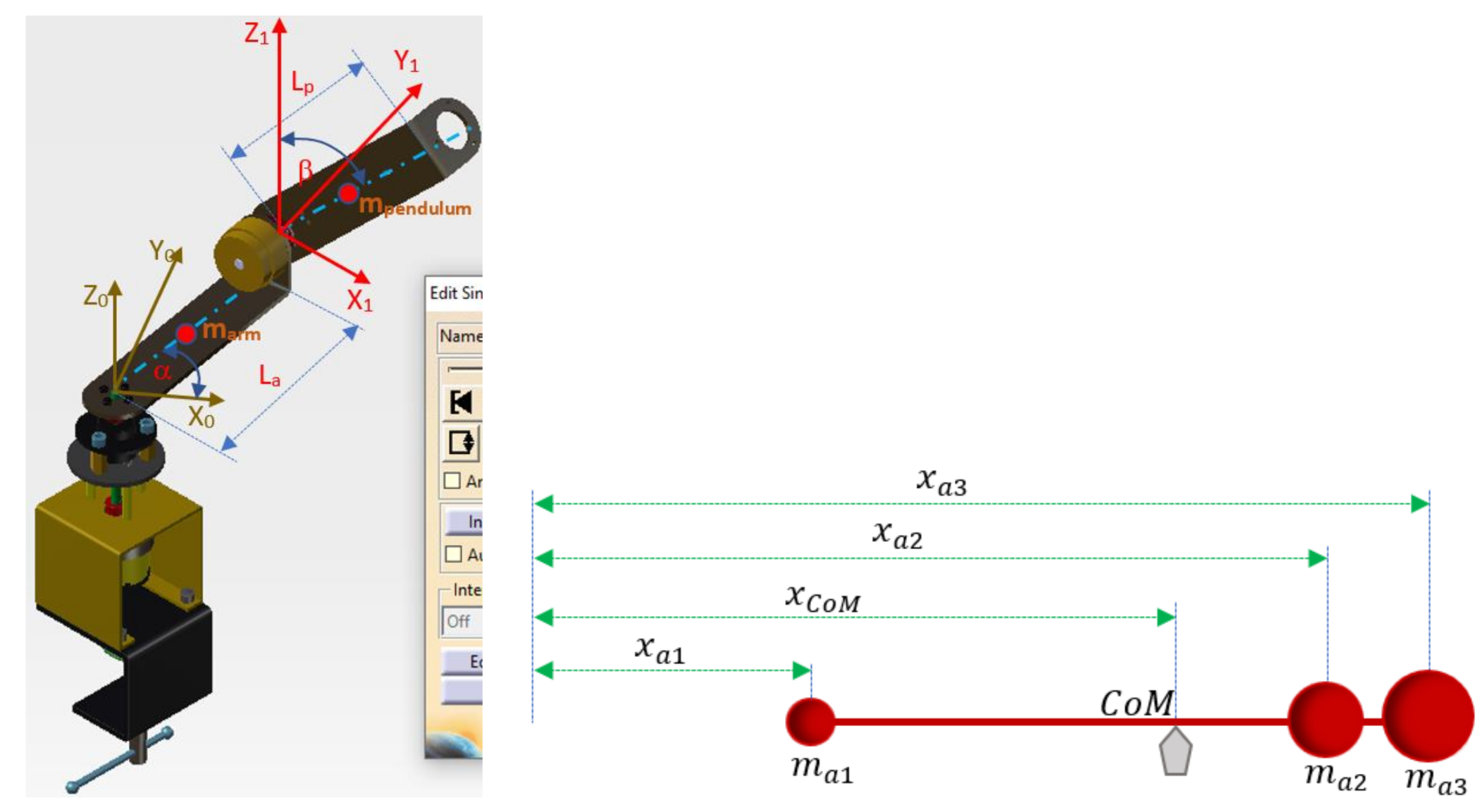
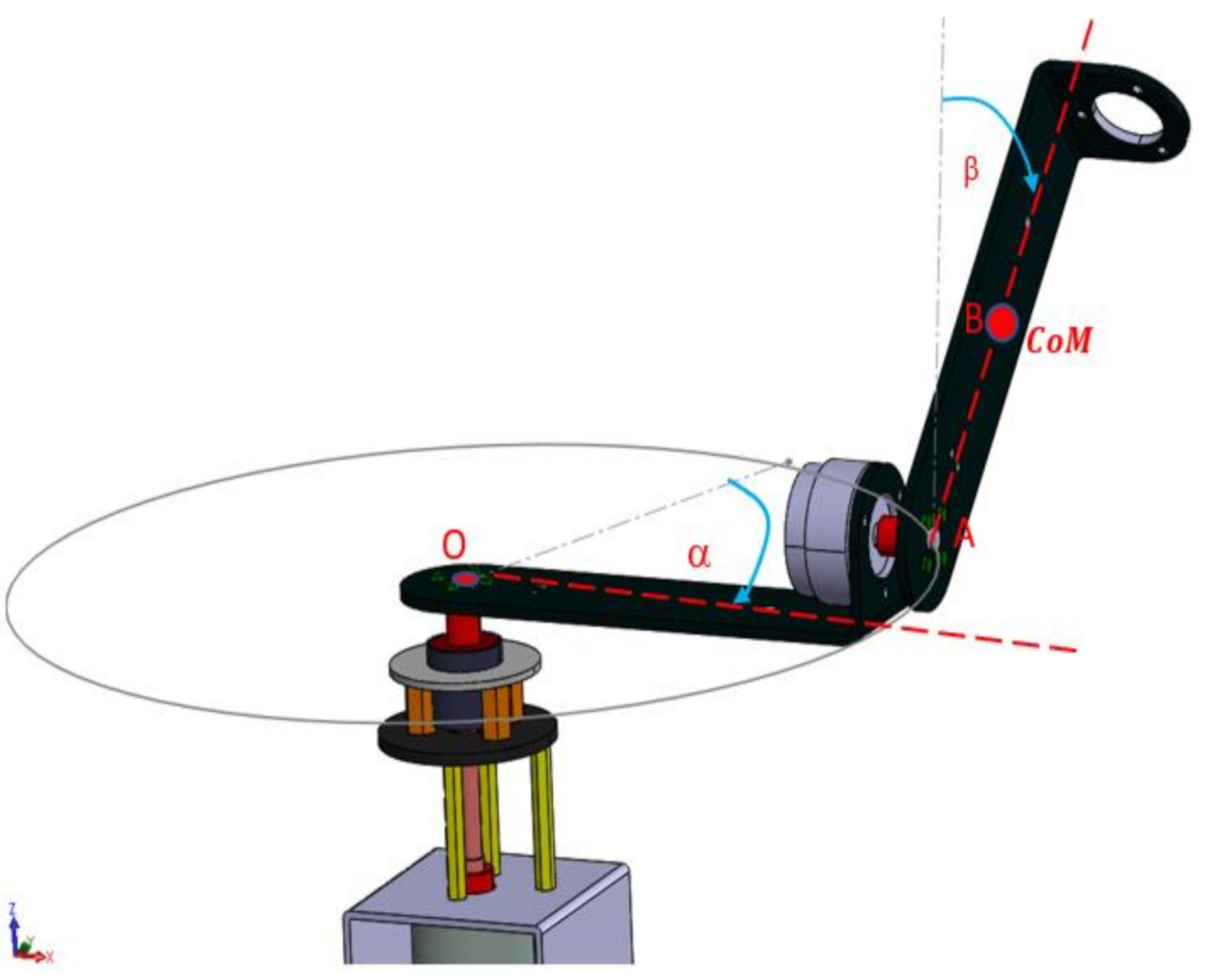
2. Rotary Inverted Pendulum

The model of rotational link 2 is shown in Figure 2. The rotating joint is appended to the servo engine shaft. The pivoting arm [rotating link] has a length, L_arm a moment of inertia, J_arm and an angle α; α increments decidedly when turning the counterclockwise. The pendulum interface is associated with the finish of the pivoting joint. It has an all-out connection L_pend and a focal point of mass m_pend. The moment of inertia for its center of mass is J_pend. The angle of inverted link 2, β, is zero when the inverted arm is in an upright position; by dividing the symmetry space along the z axis, and it increases in the positive direction when it moves in the clockwise direction [18,21]. There are six main components of the RIP, as shown in Figure 1: link 2, link 1, a motor with a gearbox ratio of 20:1, a base, and two encoders [1]. The RIP system is depicted in Figure 1, along with the geometric parameters and system variables.

The RIP has two planes of symmetry through the z₀ axis with a normal direction of x₀ and y₀; it can rotate in the plane perpendicular to l_a = y₁.

This is attributed to its symmetrical configuration. Therefore, the distance x_CoM from the centre of mass (CoM) can be calculated as follows:

$${\mathrm{x}}_{\mathrm{CoM}}=\frac{{{\displaystyle \sum }}_{\mathrm{i}=1}^{\mathrm{n}}{\mathrm{m}}_{\mathrm{i}}·{\mathrm{x}}_{\mathrm{i}}}{{{\displaystyle \sum }}_{\mathrm{i}=1}^{\mathrm{n}}{\mathrm{m}}_{\mathrm{i}}}=\frac{m_{a1}·x_{a1}+m_{a2}·x_{a2}+m_{a3}·x_{a3}}{m_{a1}+m_{a2}+m_{a3}}$$

(1)

$x_{CoM}$ distance from some reference point to the (CoM), and x_i: distance to the CoM for each individual object.

The movement of the mechanism can be described in a graph-analytical or analytical manner.

From Figure 2 is derived the kinematics equation of link 2.

$$\overrightarrow{{\mathrm{r}}_{\mathrm{B}/\mathrm{A}}}=\frac{1}{2}·{\mathrm{L}}_{\mathrm{pend}}·\left(-\sin \mathsf{\beta }·\overrightarrow{ı}+\cos \mathsf{\beta }·\overrightarrow{ȷ}\right)$$

(2)

$$\overrightarrow{{\mathrm{v}}_{\mathrm{B}/\mathrm{A}}}=\frac{1}{2}\mathsf{·}{\mathrm{L}}_{\mathrm{pend}}·-\cos \mathsf{\beta }·\dot{\mathsf{\beta }}·\overrightarrow{ı}-\sin \mathsf{\beta }·\dot{\mathsf{\beta }}·\overrightarrow{ȷ})$$

(3)

$$\overrightarrow{{\mathrm{v}}_{\mathrm{A}/\mathrm{O}}}={\mathrm{L}}_{\mathrm{arm}}·\dot{\mathsf{\alpha }}·\overrightarrow{ı}$$

(4)

$$\overrightarrow{{\mathrm{v}}_{B/O}}=\overrightarrow{{\mathrm{v}}_{B/A}}+\overrightarrow{{\mathrm{v}}_{A/O}}=\left({\mathrm{L}}_{\mathrm{arm}}·\dot{\mathsf{\alpha }}-\frac{1}{2}·{\mathrm{L}}_{\mathrm{pend}}·\cos \mathsf{\beta }\right)·\overrightarrow{ı}-\frac{1}{2}·{\mathrm{L}}_{\mathrm{pend}}·\dot{\mathsf{\beta }}·\sin \mathsf{\beta }·\overrightarrow{ȷ}$$

(5)

The Kalman filter is moderately less numerically confounded and simpler to use than the other filters, for example, the applied filter. Therefore, the limit of the Kalman filter to situate nonlinear coordinated frameworks precisely is restricted [19,23,24,25]. The all-inclusive Kalman filter is expressed in Algorithm 1. In the accompanying Figure 3 and Figure 4, we applied the Kalman filter on the grounds that the clamours from the encoder were enormous.

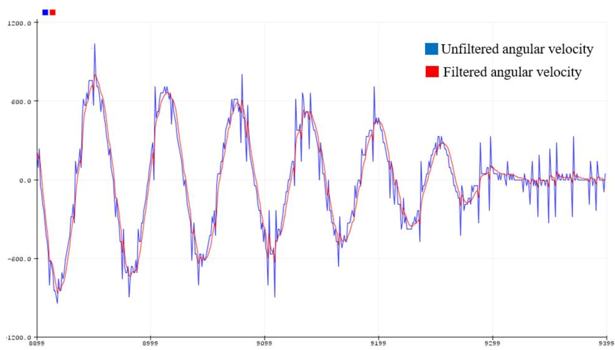
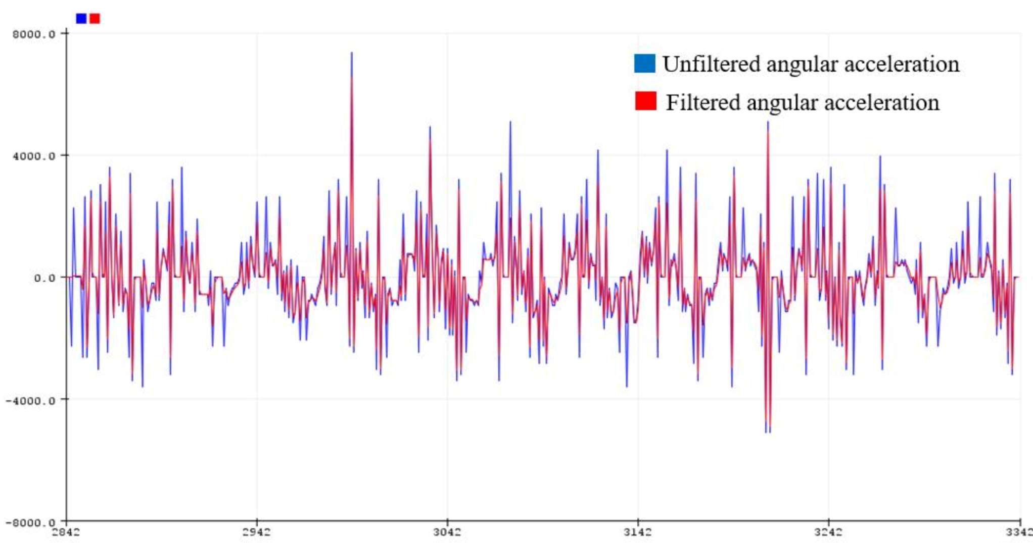
Algorithm 1 Description of the filtered angular velocity/acceleration.
Input: angular position, angular velocity, angular acceleration Output: $u_{\beta }$
for $u_{\beta } \in angular data do$
	$\mathsf{\beta }=P_{pend\text{-}pred}{C}^T{\left(C·P·C^T+R\right)}^{-1}$
	$\widehat{x_{\mathsf{\beta }}}=angula{r}_{k-1}+\mathsf{\beta }·\left(\mathrm{y}\left(\mathrm{k}-1\right)-C·angula{r}_{k-1}\right)$
	$P=\left(I-\beta ·C\right)·L_{pend}$
	$angula{r}_k=discrete our model\left(\widehat{x_{\mathsf{\beta }-1},}{u}_{\beta -1}\right)$
	${\mathrm{F}}_{\beta }=\frac{\partial discrete our model}{\partial x}{\left.\begin{array}{c}\\ \end{array}\right|}_{\widehat{x_{\mathsf{\beta }-1},}{u}_{\beta -1}}$
	$P_{pend\text{-}pred}$= ${\mathrm{F}}_{\beta }·L·{\mathrm{F}}_{\beta }{}^T+Q$
end

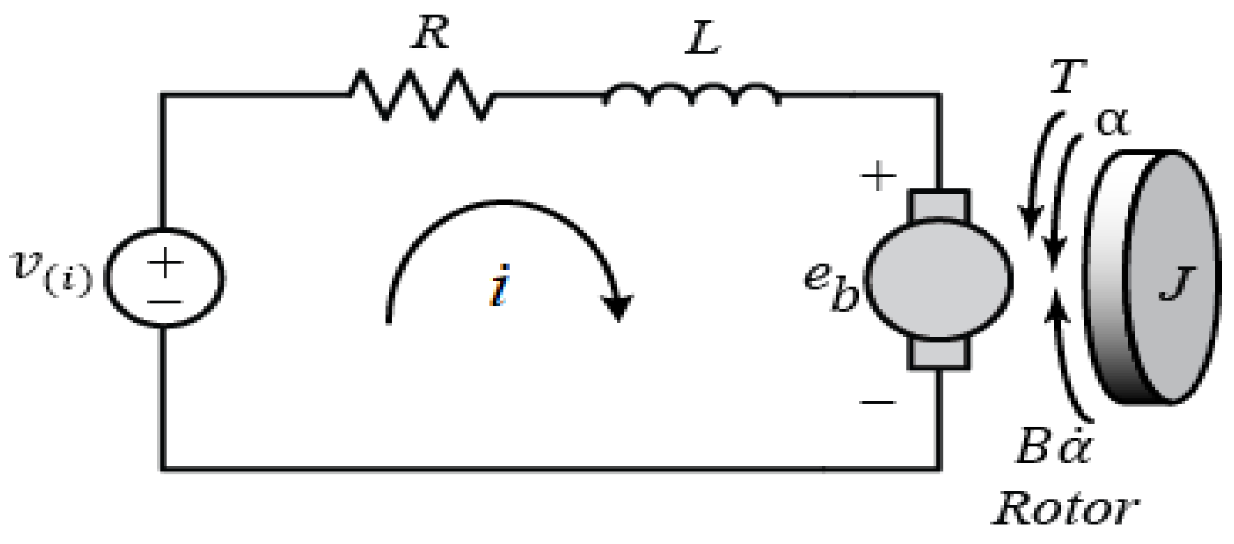
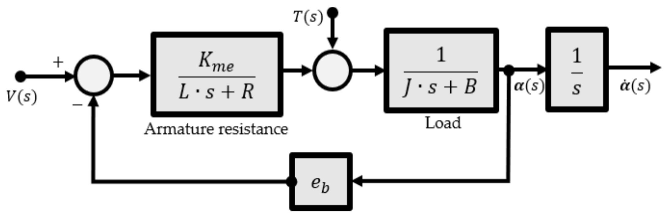
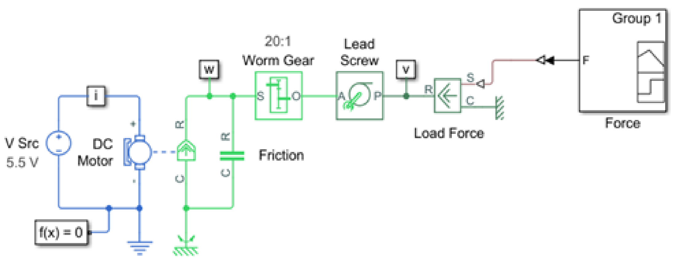
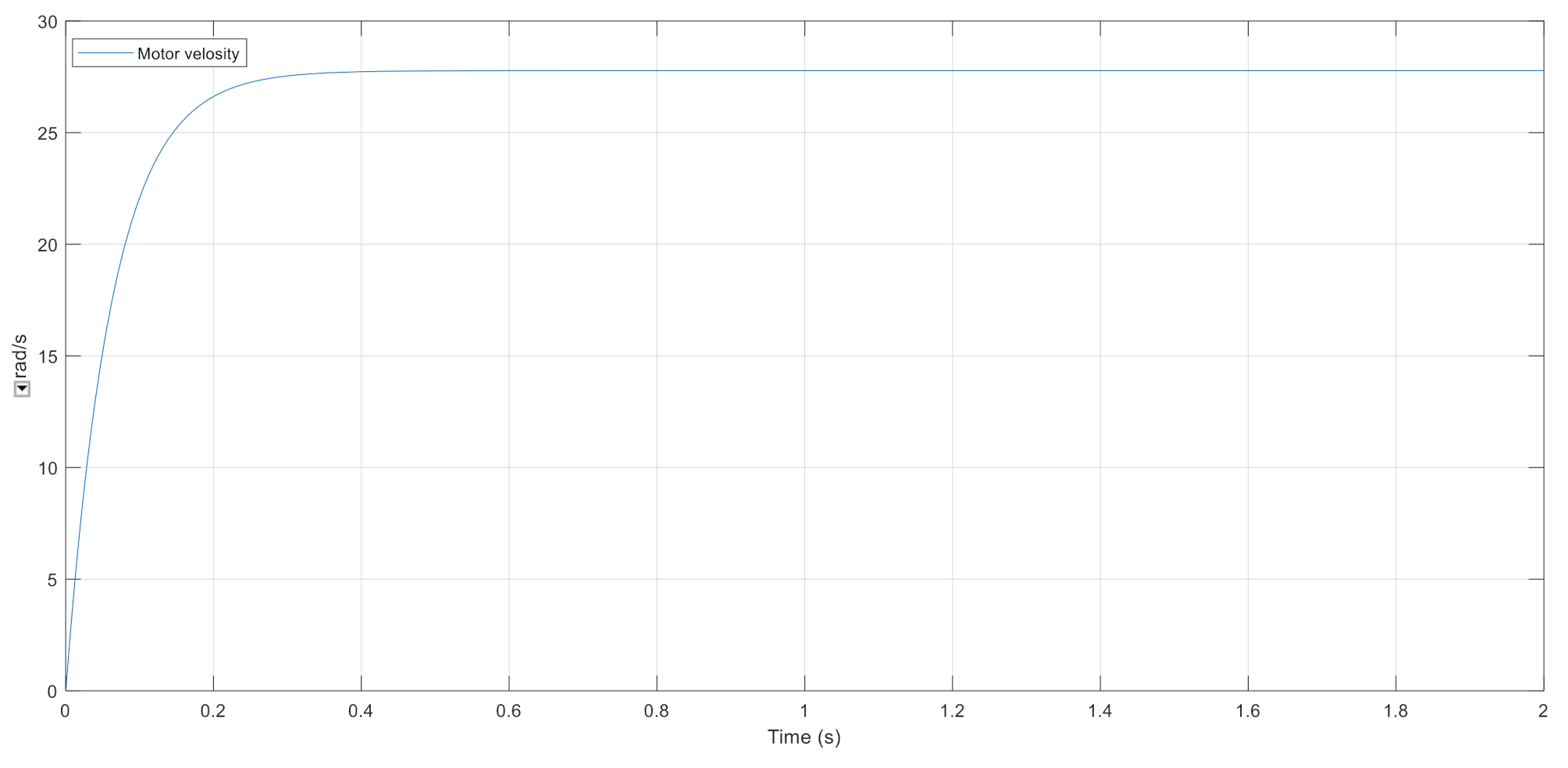
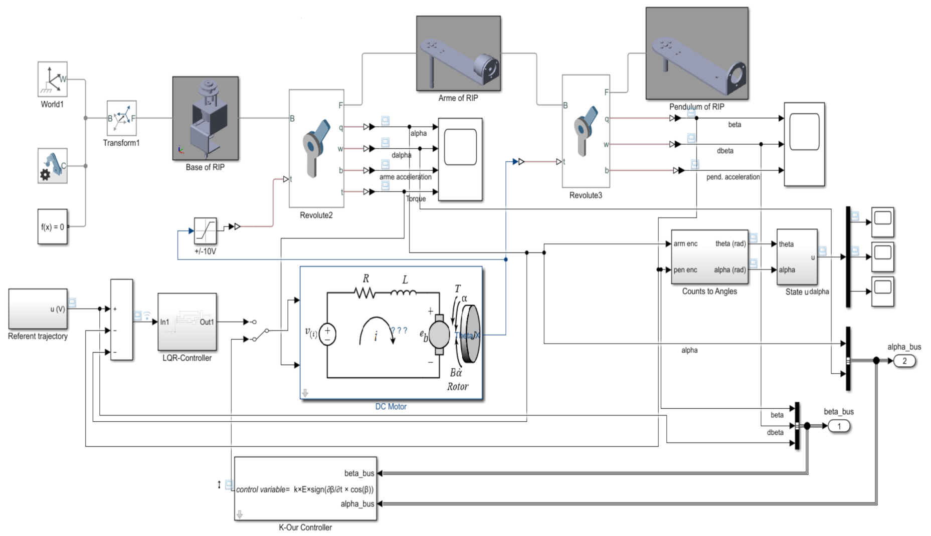
3. DC Motor Modelling

The electric equal circuit of the armature and the free-body chart of the rotor are shown in Figure 5.

The input of the system is the feeding voltage (v) applied to the motor’s armature. The system output is the angular velocity of the shaft, marked as ${\dot{\alpha }}_{\left(t\right)}$ [20].

Therefore, we measured two parameters: armature resistance R and torque constant K_me. From the measured samples for the R, we took 30 measurements, and their average was R = 9.59 Ω.

$$v_i\left(t\right)=i\left(t\right)·L\frac{di}{dt}+R·i\left(t\right)+e_b\left(t\right)$$

(6)

$$\mathrm{T}=B\frac{d\alpha }{dt}+J·\frac{d^2\alpha }{d{t}^2}$$

(7)

$$e_b=K_{me}·{\dot{\alpha }}_{\left(t\right)}$$

(8)

$$T=K_{me}·i\left(t\right)$$

(9)

Upon applying the Laplace transform to Equations (6)–(9), we obtained the following expressions in the frequency domain:

Where: ${\dot{\alpha }}_{\left(t\right)}={\omega }_{\left(t\right)}={\mathsf{\Omega }}_{\left(s\right)}$, ${\ddot{\alpha }}_{\left(t\right)}={\dot{\omega }}_{\left(t\right)}=\mathrm{s}·{\mathsf{\Omega }}_{\left(s\right)},$ $v_i\left(t\right)=V_i\left(s\right)$ and $i\left(t\right)$ = ${\mathrm{I}}_{\left(s\right)}$.

$$\frac{{\mathsf{\Omega }}_{\left(s\right)}}{V_i\left(s\right)}=\frac{{\mathrm{K}}_{\mathrm{me}}}{\mathrm{J}·\mathrm{L}·{\mathrm{s}}^2+\left(\mathrm{J}·\mathrm{R}+\mathrm{L}·\mathrm{B}\right)·\mathrm{s}+\mathrm{R}·\mathrm{B}+{\mathrm{K}}_{\mathrm{me}}{}^2}$$

(10)

The differential conditions from above can likewise be communicated in the state-space structure by selecting the engine position, engine speed, and armature current as the state variables [7]. Let the variables be $\frac{d{\dot{\alpha }}_{\left(t\right)}}{dt}={\ddot{\alpha }}_{\left(t\right)}=-\frac{\mathrm{B}}{\mathrm{J}}·{\dot{\alpha }}_{\left(t\right)}-\frac{{\mathrm{K}}_{\mathrm{me}}}{\mathrm{J}}·i\left(t\right) \mathrm{and} \frac{di\left(t\right)}{dt}=-\frac{{\mathrm{K}}_{\mathrm{me}}}{\mathrm{L}}·{\dot{\alpha }}_{\left(t\right)}-\frac{\mathrm{R}}{\mathrm{L}}·i\left(t\right)+\frac{1}{\mathrm{L}}·v_i\left(t\right)$; it is not difficult to get the accompanying state-space structure to depict in a linear form for the input and the output.

$$\frac{d}{dt}·\left.\left[\begin{array}{c}{\dot{\alpha }}_{\left(t\right)}\\ i\left(t\right)\end{array}\right]=\left[\begin{array}{cc}-\frac{B}{J}& -\frac{{\mathrm{K}}_{\mathrm{me}}}{J}\\ -\frac{{\mathrm{K}}_{\mathrm{me}}}{L}& \frac{R}{L}\end{array}\right]·\left[\begin{array}{c}{\dot{\alpha }}_{\left(t\right)}\\ i\left(t\right)\end{array}\right]+\left[\begin{array}{c}0\\ \frac{1}{L}\end{array}\right]·v_i\left(t\right); \mathrm{y}\left(\mathrm{t}\right)=\left[\begin{array}{cc}1& 0\end{array}\right]·\left[\begin{array}{c}{\dot{\alpha }}_{\left(t\right)}\\ i\left(t\right)\end{array}\right]\right\}$$

(11)

Figure 6 presents a scheme of the DC motor with feedback control, and Figure 7 shows the DC motor simulation with the real parameters by using MATLAB/Simscape. The block diagram of Figure 6 has been included within the Simscape/Simulink in the DC motor block of Figure 7, in particular.

It has been proven for the RIP’s equation of motion that the symmetry leads to the possibility of obtaining the solutions by using a real-time variable.

The steady-state velocities with different voltages obtained from the Simulink modes are shown in Figure 8.

The steady-state velocities with different voltages obtained from the real DC motor are shown in Figure 9.

4. Rotary Inverted Pendulum Dynamics

Mathematical modelling should be possible by utilizing the Euler–Lagrange strategy. In order to write the differential equations of the motion of the pendulum [31], taking into consideration the symmetry between two links, we started from the general form of the Lagrange equations of the second type.

$$\begin{array}{c}L=\frac{1}{2}·m_{pend}{\left(\frac{L_{arm}}{2}\right)}^2·{\dot{\alpha }}^2+\frac{1}{2}·J_{arm}·{\dot{\alpha }}^2+1/2·[L_{arm}^2·{\dot{\alpha }}^2+{\left(\frac{L_{pend}}{2}\right)}^2·{\dot{\beta }}^2+{\left(\frac{L_{pend}}{2}\right)}^2·si{n}^2\beta ·{\dot{\alpha }}^2\\ +L_{arm}·L_{pend}·\cos \alpha ·\dot{\alpha }·\dot{\beta }]+\\ \frac{1}{2}·J_{pend}·{\dot{\beta }}^2-\left(m_{arm}+m_{pend}\right)·\mathrm{g}·\mathrm{h}-\frac{1}{2}·m_{pend}·L_{pend}·\mathrm{g}·\cos \beta \end{array}$$

(12)

$$\frac{d}{dt}\left(\frac{\partial L}{\partial \dot{\alpha }}\right)-\frac{\partial L}{\partial \alpha }=\tau ,\frac{d}{dt}\left(\frac{\partial L}{\partial \dot{\beta }}\right)-\frac{\partial L}{\partial \beta }=0$$

(13)

From Equations (11) and (12) we derived the followings:

$$\begin{array}{c}{m}_{arm}{\left(\frac{L_{arm}}{2}\right)}^2·\ddot{\alpha }+J_{arm}·\ddot{\alpha }+J_{arm}·L_{arm}{}^2\ddot{\alpha }+m_{pend}{\left(\frac{L_{arm}}{2}\right)}^2·si{n}^2\beta ·\ddot{\alpha }+m_{pend}{L_{arm}}^2+\\ \sin \beta ·\cos \beta ·\dot{\alpha }·\dot{\beta }+\frac{1}{2}·m_{pend}·L_{pend}·L_{arm}·\cos \beta ·\ddot{\beta }-\frac{1}{2}·m_{pend}\\ ·L_{pend}·L_{arm}·\sin \beta ·{\dot{\beta }}^2=\tau \\ m_{pend}{\left(\frac{L_{pend}}{2}\right)}^2·\ddot{\beta }+J_{arm}·\ddot{\alpha }+\frac{1}{2}·m_{pend}·L_{pend}·L_{arm}·\cos \beta ·\ddot{\beta }-\frac{1}{2}·m_{pend}·L_{pend}{}^2\\ ·\cos \beta ·\sin \beta ·{\dot{\alpha }}^2-\frac{1}{2}·m_{pend}·L_{pend}·\mathrm{g}·\sin \beta =0\end{array}\},$$

(14)

$q=\left[\alpha , \beta \right]$ => $\dot{q}=\left[\dot{\alpha }, \dot{ \beta }\right]$—controllable variables—equal to the degrees of freedom. As we had two controllable variables, the two degrees of freedom, respectively, in the matrix form will be as follows:

$$D\left(q\right)\cdot \ddot{q}+H\left(q,\dot{q}\right)+G\left(q\right)=\tau$$

(15)

where: $D\left(q\right)$—kinetic energy matrix, $H\left(q,\dot{q}\right)$—centrifugal and Coriolis forces, $\mathrm{G}\left(\mathrm{q}\right)$—gravitational forces, and $\tau$—torque.

The required partial derivatives for substitution in Equations (13)–(15) are as follows:

$$D\left(q\right)=\left[\begin{array}{cc}{J}_{arm}+m_{pend}·L_{arm}^2+m_{pend}·L_{pend}^2·sin\beta & m_{pend}·L_{arm}·L_{pend}·cos\beta \\ m_{pend}·L_{arm}·L_{pend}·cos\beta & J_{pend}+m_{pend}·L_{pend}^2\end{array}\right]$$

(16)

$$H\left(q,\dot{q}\right)\left[\begin{array}{cc}\frac{L_{arm}}{2}+\frac{m_{pend}}{2}·L_{arm}^2+m_{pend}·L_{pend}^2·\dot{\beta }·sin2\beta & +\frac{m_{pend}}{2}·L_{pend}^2·\dot{\alpha }·sin2\beta -\Gamma \\ \frac{m_{pend}}{2}·L_{pend}^2·sin2\beta & \frac{L_{pend}}{2}\end{array}\right]$$

(17)

where: $\Gamma =m_{pend}·L_{pend}·\dot{\alpha }·sin\beta$

$$G\left(q\right)=\left[\begin{array}{c}0\\ m_{pend}{L}_{pend}^2·g·sin\beta \end{array}\right],$$

(18)

$$\tau =\frac{K_{me}}{\mathrm{R}}\mathrm{V}-\frac{K_{me}{}^2}{\mathrm{R}}·\dot{\alpha }$$

(19)

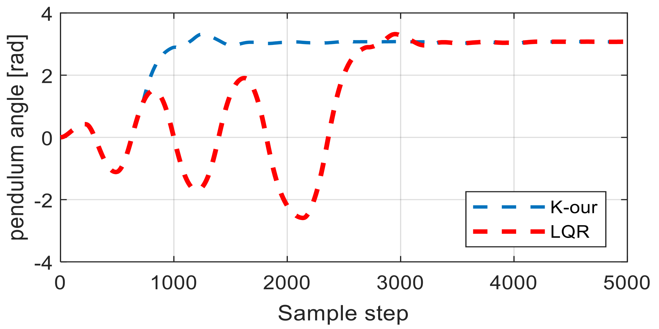
5. Swing-Up and Stabilisation of RIP

The descending position to the vertical upright position and to hold it there. We used two control strategies: one for swinging up, and the other for balancing the pendulum parts with a small error to reach the dead position as soon as possible. The control using sliding models [32] was developed for both the methods of swinging up and stabilising $𝓏={𝓀}^{\mathcal{T}}{𝓏}_{ℯ}$. A subsequent order system for position control with a swaying joint movement that went about as the disturbance was mulled over for the pendulum of the swing up control. The following controller was structured with the goal that it followed a reference input in our case with a reference trajectory. Because of the symmetrical configuration of the RIP, this provided energy to the swing joint and placed it at the focal point, where it was utilised in another pendulum balancing control to balance out the unsteady points. For the trajectory, the quadrilateral wave of amplitude ±π/6 was used. The state-space equation for the stance control system [33] used was $\dot{𝓏}=\mathcal{A}·𝓏+\mathcal{B}·u+\mathcal{D}$, where the variables $\mathcal{A}$ and $B$ are the system matrix and $D$ is a concentrated disturbance that contains a disturbance due to an oscillating connection of the pendulum. Thus, ${𝓏}_e\in \left(ℯ,{\dot{ℯ}}_z\right)$ represented the error state vector, the desired state vector was $z_d$, and the actual state vector was ${𝓏}_e=\left(𝓏-{𝓏}_d\right)$. The equation $\dot{𝓏}=\Pi ·{\left|𝓏\right|}^{\beta }·sign\left(𝓏\right)$ used differentiating sliding models $\dot{𝓏}={𝓀}^{\mathcal{T}}{\dot{𝓏}}_{ℯ}$, and then, we substitute the actual state vector ${\dot{𝓏}}_e=\left(\dot{𝓏}-{\dot{z}}_d\right)$. Thus, we obtained the sliding model $\dot{𝓏}={𝓀}^{\mathcal{T}}\left(\dot{z}-{\dot{z}}_d\right)$. If $z_d\in \left(\pm \frac{\pi }{6},0\right)$ was the desired vector, the derivative vector was ${\dot{z}}_d\in \left(0,0\right)$. The conditions given above were to integrate the control $u=-\frac{1}{{𝓀}^{\mathcal{T}}\mathcal{B}}·\left[{𝓀}^{\mathcal{T}}\mathcal{A}·z+\mathsf{\Pi }·{\left|z\right|}^{\beta }·sign\left(z\right)\right]$; it was swing-up control, and the exchanging gain $\Pi$ was more noteworthy than the greatest furthest reaches of the ${𝓀}^{\mathcal{T}}\mathcal{D}$ guarantee sliding [32]. The RIP system was a fourth-order system, and the state space was obtained with Equations (6) and (15), where $z\in {\mathcal{R}}^{4x1}, \mathcal{A}\in {\mathcal{R}}^{4x4}$, and $\mathcal{B}\in {\mathcal{R}}^{4x1}$. On the basis of the above equation, the incorporated control was $u=-\frac{1}{{𝓀}^{\mathcal{T}}\mathcal{B}}·\left[{𝓀}^{\mathcal{T}}\mathcal{A}·z+\mathsf{\Pi }·{\left|z\right|}^{\beta }·sign\left(z\right)-{𝓀}^{\mathcal{T}}{\dot{z}}_d\right]$ and the swing up control is presented.

6. Simulation Results

The simulation is shown in Figure 10, using $K_{our}$ and the LQR controller. For our controller, the parameters used were $K_{our}=\left[2, 4, 6, 10\right]$. The indicial parameter for $K_{LQR}$ was $K_{LQR}=\left[-381.5,-26.7, 3.08, 12.25\right]$. The parameter of LQR was as follows: $u=-5200$, $if 0<\beta \le -90$°, $\alpha \ge 0$ and $u=5200$, $if-90<\beta \le 0$°, $\alpha \le 0$, and $Q=diag\left(90, 10, 40, 50\right)$.

The reactions of the link 2 angle obtained by, respectively, utilising our strategy and the LQR method are presented in Figure 11, from which, one can infer that our swing-up technique was quicker than that utilising the LQR control scheme. The explanation was that, in the LQR control technique, link 2 needed to follow a to-and-fro movement until it arrived at a little neighbourhood of the vertical position [1]. Such a strategy would cost a considerable amount of time. Moreover, in our method, link 2 could be swung up with less movement because of the high-efficiency utilisation of the inertia [1]. Note that the multi-switching of the LQR controller might cause harm to the motor. In any case, the switching recurrence of our controller was considerably less than that of the LQR controller. A detailed performance comparison of our method and the LQR scheme is presented in

Table 1. Simulation performance analyses.

Definition	Unit	Kour Cont.	Cont. [1]	LQR Cont.	LQR Cont. [1]
Swing up and stabilisation time	s	1.53	5.4	3.35	15
Steady-state error	rad	0.01	0.1	0.2	0.2
Controller saturation time	s	0.003	0.005	9	13

, along with the swing up time, steady-state error, controller switched times, and controller saturation time [1] of our method; all of them were less than those of the LQR scheme. This detailed performance comparison revealed that our method was more efficient in terms of the swing up time and stabilisation for the same RIP.

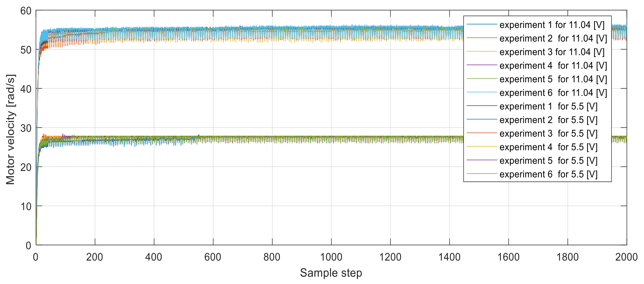
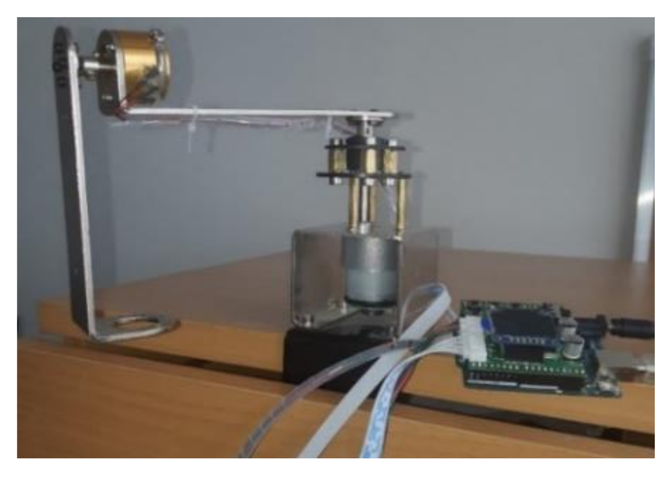
7. Experimental Results

This section shows the experimental results of the combined sensitivity of our controller in comparison with LQR [28]. The platform of the RIP system is shown in Figure 12. The main controller chip was STM32F10 and Arduino Uno, the engine was MG513IPH, and the driver IC was TB 6612FNG [1]. The parameters for our controller were as follows: $K_{our}=\left[2, 4, 6, 10\right]$. The linear feedback parameter for $K_{LQR}$ was as follows: $K_{LQR}=\left[-381.5,-26.7, 3.08, 12.25\right]$. The parameter of LQR was set as follows: $u=-5200$, $if 0<\beta \le -90$°, $\alpha \ge 0$, and $u=5200$, $if-90<\beta \le 0$°, $\alpha \le 0$, and $Q=diag\left(90, 10, 40, 50\right)$. In the following text, we present the pseudo-code Algorithms 2–4 for our swing up method and the LQR for a low-cost RIP platform.

The following algorithms of the different calculations for the RIP case are given based on their writing according to the authors [34].

Algorithm 2 Parameters and description of the calculation of angle/velocity.

Input: $n, m, R_{armature}, K_{me}, V_{out}, Xve{l}_{rad}, X_{ang},Xlas{t}_{ang}$

for $Po{s}_{old}=0:\mathrm{k}$ do if $k$= 0 or $Xve{l}_{rad}$ > −1 and $X_{ang}\ge Xve{l}_{rad}$ then $Po{s}_{old}=\left( Xlas{t}_{ang}-star{t}_{Ang}\right)$//$⊳$ calculate the pendulum angle end if if $k>0$ then      $Xve{l}_{rad}= (X_{ang}-Xlas{t}_{ang})$//$⊳$ calculate the pendulum velocity else //$⊳$ use last velocity updated $Xve{l}_{rad}$

end if end for end Output: $u_{\beta }$

Algorithm 3 Description of the calculation parameteres for swing up.

Input: $vel,n,m, las{t}_{vel}, ve{l}_{Rad};ang, las{t}_{ang}, star{t}_{Ang}, a_{cc}$ for l = 0:k do if k = 0 or $x_{vel}>-1 and l\ge x_{vel}$ then $x_{vel}=vel-las{t}_{vel}//⊳$ use last updated. ang = $las{t}_{ang}-n//⊳ \mathrm{function} \mathrm{constraining} \mathrm{the} \mathrm{angle} \mathrm{between} -\mathsf{\pi } \mathrm{and} \mathsf{\pi }$. end if if k > 0 then      $Kalma{n}_{estim.}=estim{.}_{Error}+Kalma{n}_{gain}\ast \left(Mea{s}_{curr.}-las{t}_{Estim.}\right)$ ang = $(las{t}_{ang}-\pi )\ast m//⊳$ the calculation parameters for swing up end if end for

end Output: $ne{w}_{pos.}//⊳$ through position we control the angle of the pendulum

Algorithm 4 Calculation of potential energy and torque.

$\mathrm{Input}: E_k,E_p, m_{pend}, L_{pend}, x_{spd}, m_{arm}, L_{arm}, n, m, T_m$ for l = 0:k do if $\mathrm{k}=0\hspace{1em}\mathrm{or}\hspace{1em}an{g}_{rad.}>1$$\hspace{1em}\mathrm{and}\hspace{1em}l\ge an{g}_{rad.}\hspace{1em}\mathrm{then}$ $X_{ang}=n\ast \left(ol{d}_{pos.}-ol{d}_{curr}.\right)//⊳ \mathrm{shift} \mathrm{of} \mathrm{the} \mathrm{angle}$ end if if k > 0 then $x_{velRad}=m\ast \left( X_{ang}-X_{lastAng}.\right);//⊳ \mathrm{new} \mathrm{shif} \mathrm{of} \mathrm{the} \mathrm{pendulum} \mathrm{angle}$ $E_p=-m_{pend.}\ast g\ast L_{pend.}(1-\cos (an{g}_{rad.}$$)//⊳ \mathrm{calculate} \mathrm{potential} \mathrm{energy}$ else $//⊳$$\mathrm{use} \mathrm{last} \mathrm{updated}\hspace{1em} x_{velRad}$ end if $\mathrm{if}\hspace{1em} anl{.}_{Read.}\ne 0\hspace{1em}\mathrm{then}$ $ang=n\ast \hspace{1em}anl{.}_{Read.}+m//⊳$$\mathrm{pendulum} \mathrm{angle} \mathrm{for} \mathrm{swing} \mathrm{up}\hspace{1em}\beta \approx \pi$ end if $\mathrm{if}\hspace{1em} x_{spd}>0\hspace{1em}\mathrm{then}$ $x_{spd}=ang\ast K_{me}+m;//⊳ \mathrm{calculate} \mathrm{of} \mathrm{the} \mathrm{speed}$ end if $T_m=(x_{spd}\ast V_{out-max})/ve{l}_{max}//⊳ \mathrm{calculation} \mathrm{of} \mathrm{the} \mathrm{torque} \mathrm{for} \mathrm{the} \mathrm{swing} \mathrm{up}$ end for

end $\mathrm{Output}\hspace{1em}\beta \approx \pi$$\hspace{1em}\mathrm{and}\hspace{1em}{T}_m$

The experimental results are shown in Figure 12, Figure 13, Figure 14, Figure 15, Figure 16, Figure 17 and Figure 18. Figure 12 shows the responses of the pendulum angle, Figure 13 shows the responses of the pendulum angle velocity $\dot{\mathit{\beta }}$, Figure 14 shows the responses of the pendulum acceleration swing unfiltered $\ddot{\mathit{\beta }}$, and Figure 15 shows the response of the arm velocity $\dot{\mathit{\alpha }}$; these data are presented in the sample steps. The response of the controller is given in Figure 16. Figure 17 shows that link 2 swung up in approximately 1.45 s for ${\mathit{K}}_{\mathit{o}\mathit{u}\mathit{r}}=\mathbf{10}$, and then was stabilised by the control. It is clearer from Figure 18 that the nonlinear part of the stabilisation controller worked from less than 1000 sample steps to 5000 sample steps under our controller for ${\mathit{K}}_{\mathit{o}\mathit{u}\mathit{r}}=\mathbf{10}$, roughly. Note that all the signals of the RIP were stable. Furthermore, the swing up and equilibration time, steady-state error, and controller response time are presented in

Table 2. Experimental performance analyses.

Definition	Unit	Data
Swing up and stabilisation time	s	1.45
Extreme force	N	2.23
Steady-state error	rad	0.03
Controller saturation time	s	0.001

below. Link 2′s angle $\mathit{\beta }$ position and link 1′s arm position α were in symmetry.

Figure 13 shows the reduced time for the swing up and stabilisation. The best value was observed in the case of ${\mathit{K}}_{\mathit{o}\mathit{u}\mathit{r}}=\mathbf{10};$ we observed that for the swing up, it took less than 1500 sample steps to get the pendulum angle in the vertical position. The worst value was obtained in the case of ${\mathit{K}}_{\mathit{o}\mathit{u}\mathit{r}}=\mathbf{2};$ here, we observed that the swing up and stabilisation took more than 3500 sample steps to get the pendulum angle in the vertical position.

Figure 14 shows the reduced time for the swing up and stabilisation. The best value was obtained in the case of ${\mathit{K}}_{\mathit{o}\mathit{u}\mathit{r}}=\mathbf{10};$ here, we observed that for the swing up, it took less than 1000 sample steps to get the pendulum angle in the vertical position. The worst values were obtained in the case of ${\mathit{K}}_{\mathit{o}\mathit{u}\mathit{r}}=\mathbf{4}$ and ${\mathit{K}}_{\mathit{o}\mathit{u}\mathit{r}}=\mathbf{2},$ as the swing up and stabilisation took more than 1800 sample steps to get the pendulum velocity in the vertical position.

Hence, we reduced the time required for the swing up and stabilisation. The best value was obtained in the case of ${\mathit{K}}_{\mathit{o}\mathit{u}\mathit{r}}=\mathbf{10}$; we observed that for the swing up, it took less than 800 sample steps to get the pendulum angle in the vertical position. The worst value was obtained in the case of ${\mathit{K}}_{\mathit{o}\mathit{u}\mathit{r}}=\mathbf{2};$ here, we observed that the swing up and stabilisation took more than 1000 sample steps to get the pendulum angle in the vertical position. Hence, Figure 15 shows the reduced time taken for the swing up and stabilisation. The best value was obtained in the case of ${\mathit{K}}_{\mathit{o}\mathit{u}\mathit{r}}=\mathbf{10}$; we observed that for the swing up, it took less than 870 sample steps and the potential energy in the y direction was −655.84 to give the pendulum potential energy in vertical position up, technique reaction, and the adjustment procedure reaction of the RIPS by utilising the structured swing-up control.

The worst values were obtained in the case of ${\mathit{K}}_{\mathit{o}\mathit{u}\mathit{r}}=\mathbf{2}$; we observed that the swing up and stabilisation took more than 1177 sample steps and the potential energy in the y direction was −424.69. The experiment exhibited the whole procedure of the dynamic reaction including the swing.

Figure 19 shows the motions of the RIP, in which 1, 2 illustrate the amplitude-increased simple pendulum motion, 3–5 demonstrate the swing up condition, 6–7 show the inertia swing up procedure, and 11–15 depict the stabilisation process. Figure 19 shows the caught movements of the RIPS, wherein 1–2 illustrate the amplitude-increased simple pendulum motion, 3–5 exhibits the swing up condition, 6, 7 show the inertia swing up technique, and 11–15 describe the stabilisation procedure.

8. Conclusions

In this paper, the control schemes for the RIP system that could be used to swing up the pendulum and balance it in the upright position were presented. A benchmark control, namely control of an RIP system, using sliding control was investigated. The position control of the arm coupled to the shaft of the actuator with sliding mode control was analysed, because of the symmetrical configuration, and to achieve the desired swing up from the RIP system’s position down has been used, to bring the pendulum into the linear range where the linear model is valid for control created. A balancing control was additionally utilised in the linear range. The sliding mode controller offered excellent swing up control and adjustment of the vertical upstanding position. The performance of controlling the RIP framework by utilising the sliding mode control for the swing up and the sliding model control for balancing out indicated the preferred performance to that of the controller with a PD controller for swing up and the LQR controller for balancing. The swing up and balancing time of under 1.5 s in the proposed strategy contrasted with the 3–4 s in the other technique was reduced.

The experimental results closely matched the simulation results. Compared with the LQR swing up controller and the single linear equilibration controller, the proposed controller was more flexible and trustworthy.

References

1. Yang, X.; Zheng, X. Swing-Up and Stabilization Control Design for an Underactuated Rotary Inverted Pendulum System: Theory and Experiments. IEEE Trans. Ind. Electron. 2018, 65, 7229–7238. [Google Scholar] [CrossRef]
2. Davison, E.J. (Ed.) Benchmark Problems for Control System Design: Report of the IFAC Theory Committee; International Federation of Automatic Control: Laxenburg, Austria, 1990. [Google Scholar]
3. Wiener, N. Cybernetics or Control and Communication in the Animal and the Machine; Technology Press: Cambridge, MA, USA, 1948. [Google Scholar]
4. Powers, W.T.; Clark, R.K.; Mc Farland, R.L. A General Feedback Theory of Human Behavior: Part I. Percept. Mot. Skills 1960, 11, 71–88. [Google Scholar] [CrossRef]
5. Chawla, I.; Singla, A. Real-Time Control of a Rotary Inverted Pendulum using Robust LQR-based ANFIS Controller. Int. J. Nonlinear Sci. Numer. Simul. 2018, 19, 379–389. [Google Scholar] [CrossRef]
6. Johnson, T.; Zhou, S.; Cheah, W.; Mansell, W.; Young, R.; Watson, S. Implementation of a Perceptual Controller for an Inverted Pendulum Robot. J. Intell. Robot. Syst. 2020, 99, 683–692. [Google Scholar] [CrossRef] [Green Version]
7. Ismail, J.; Liu, S. Efficient Planning of Optimal Trajectory for a Furuta Double Pendulum Using Discrete Mechanics and Optimal Control. IFAC-PapersOnLine 2017, 50, 10456–10461. [Google Scholar] [CrossRef]
8. Saleem, O.; Mahmood-Ul-Hasan, K. Robust stabilisation of rotary inverted pendulum using intelligently optimised nonlinear self-adaptive dual fractional-order PD controllers. Int. J. Syst. Sci. 2019, 50, 1399–1414. [Google Scholar] [CrossRef]
9. Wen, J.; Shi, Y.; Lu, X. Stabilizing a Rotary Inverted Pendulum Based on Logarithmic Lyapunov Function. J. Control Sci. Eng. 2017, 2017, 1–11. [Google Scholar] [CrossRef]
10. Wang, J.-J. Simulation studies of inverted pendulum based on PID controllers. Simul. Model. Pract. Theory 2011, 19, 440–449. [Google Scholar] [CrossRef]
11. Prasad, L.B.; Tyagi, B.; Gupta, H.O. Optimal Control of Nonlinear Inverted Pendulum System Using PID Controller and LQR: Performance Analysis Without and With Disturbance Input. Int. J. Autom. Comput. 2014, 11, 661–670. [Google Scholar] [CrossRef] [Green Version]
12. Bettou, K.; Charef, A. Control quality enhancement using fractional PIλDμ controller. Int. J. Syst. Sci. 2009, 40, 875–888. [Google Scholar] [CrossRef]
13. Dwivedi, P.; Pandey, S.; Junghare, A. Novel fractional order PDμ controller for open-loop unstable inverted pendulum system. In Proceedings of the 17th International Conference on control, Automation and Systems, Jeju, Korea, 18–21 October 2017; 2017; pp. 1616–1621. [Google Scholar]
14. Dwivedi, P.; Pandey, S.; Junghare, A. Performance analysis and experimental validation of 2-DOF fractional order controller for under actuated rotary inverted pendulum. Arab. J. Sci. Eng. 2017, 42, 5121–5145. [Google Scholar] [CrossRef]
15. Dwivedi, P.; Pandey, S.; Junghare, A.S. Stabilization of unstable equilibrium point of rotary inverted pendulum using fractional controller. J. Frankl. Inst. 2017, 354, 7732–7766. [Google Scholar] [CrossRef]
16. Dwivedi, P.; Pandey, S.; Junghare, A. Robust and novel two degree of freedom fractional controller based on two-loop topology for inverted pendulum. ISA Trans. 2018, 75, 189–206. [Google Scholar] [CrossRef] [PubMed]
17. Shang, W.W.; Cong, S.; Li, Z.; Jiang, S.L. Augmented Nonlinear PD Controller for a Redundantly Actuated Parallel Manipulator. Adv. Robot. 2009, 23, 1725–1742. [Google Scholar] [CrossRef]
18. Ozana, S.; Docekal, T.; Kawala-Sterniuk, A.; Mozaryn, J.; Schlegel, M.; Raj, A. Trajectory Planning for Mechanical Systems Based on Time-Reversal Symmetry. Symmetry 2020, 12, 792. [Google Scholar] [CrossRef]
19. Kalman, R.E. A New Approach to Linear Filtering and Prediction Problems. J. Basic Eng. 1960, 82, 35–45. [Google Scholar] [CrossRef] [Green Version]
20. Control Tutorials. University of Michigan. Available online: https://ctms.engin.umich.edu/CTMS/index.php?example=MotorSpeed&section=SystemModeling (accessed on 6 March 2021).
21. Rotary Inverted Pendulum. Available online: https://www.lehigh.edu/~inconsy/lab/css/ME389/guidelines/ME389_MEM04_PendulumGantry_Guideline.pdf (accessed on 15 May 2021).
22. Quanser. Available online: https://www.quanser.com/products/rotary-inverted-pendulum (accessed on 10 May 2021).
23. Welch, G.; Bishop, G. An Introduction to the Kalman Filter. 1995. Available online: https://www.cs.unc.edu/~welch/media/pdf/kalman_intro.pdf (accessed on 10 May 2021).
24. Vanicek, P.; Omerbasic, M. Does a navigation algorithm have to use a Kalman filter? CAASJ 1999, 45, 292–296. [Google Scholar]
25. Grewal, M.S.; Andrews, A.P. Kalman Filtering: Theory and Practice Using MATLAB, 3rd ed.; Wiley: New York, NY, USA, 2001. [Google Scholar]
26. Jadlovska, S.; Sarnovsky, J. A Complex Overview of Modeling and Control of the Rotary Single Inverted Pendulum System. Adv. Electr. Electron. Eng. 2013, 11, 73–85. [Google Scholar] [CrossRef]
27. Durand, S.; Castellanos, J.F.; Marchand, N.; Sanchez, W.F. Event-based control of the inverted pendulum: Swing up and stabilization. J. Control Eng. Appl. Inform. 2013, 15, 96–104. [Google Scholar]
28. Da Sanjeewa, S.; Parnichkun, M. Control of rotary double inverted pendulum system using mixed sensitivity H∞ controller. Int. J. Adv. Robot. Syst. 2019, 16, 1729881419833273. [Google Scholar] [CrossRef]
29. Yoshida, K. Swing-up control of an inverted pendulum by energy-based methods. In Proceedings of the 1999 American Control Conference (Cat. No. 99CH36251), San Diego, CA, USA, 2–4 June 1999; Volume 6, pp. 4045–4047. [Google Scholar]
30. Zhang, X.; Ma, J.; Lin, L.; Wang, L. Study on Swing-up Control of Rotary Inverted Pendulum Based on Energy Feedback. In Proceedings of the 2018 5th International Conference on Information Science and Control Engineering (ICISCE), Zhengzhou, China, 20–22 July 2008; pp. 994–998. [Google Scholar]
31. Guo, X.; Zhang, G.; Tian, R. Periodic Solution of a Non-Smooth Double Pendulum with Unilateral Rigid Constrain. Symmetry 2019, 11, 886. [Google Scholar] [CrossRef] [Green Version]
32. Edwards, C.; Spurgeon, S. Sliding Mode Control; CRC Press: London, UK, 1998. [Google Scholar] [CrossRef]
33. Hong, Q.; Shi, Y.; Chen, Z. Adaptive Sliding Mode Control Based on Disturbance Observer for Placement Pressure Control System. Symmetry 2020, 12, 1057. [Google Scholar] [CrossRef]
34. Tomescu, M.; Jäntschi, L.; Rotaru, D. Figures of Graph Partitioning by Counting, Sequence and Layer Matrices. Mathematics 2021, 9, 1419. [Google Scholar] [CrossRef]
Figure 1. (left) RIP system and (right) centre of mass.
Symmetry 13 01491 g001
Figure 2. Point B-CoM: centre of mass of link 2.
Symmetry 13 01491 g002
Figure 3. Pendulum angular velocity before and after Kalman filtering.
Symmetry 13 01491 g003
Figure 4. Pendulum angular acceleration before and after Kalman filtering.
Symmetry 13 01491 g004
Figure 5. DC motor in our RIP.
Symmetry 13 01491 g005
Figure 6. DC motor: mathematical model.
Symmetry 13 01491 g006
Figure 7. DC motor simulation in the MATLAB/Simscape with real parameters.
Symmetry 13 01491 g007
Figure 8. Steady-state velocities calculated from Simulink model with 5.5 V.
Symmetry 13 01491 g008
Figure 9. Steady-state velocities calculated using the average value. This is the result obtained for K values of the six experiments for 2000 samples with 5.5 V and 11.04 V.
Symmetry 13 01491 g009
Figure 10. Simulation of RIP.
Symmetry 13 01491 g010
Figure 11. RIP pendulum angle under K o u r and the LQR controller.
Symmetry 13 01491 g011
Figure 12. RIP experimental platform.
Symmetry 13 01491 g012
Figure 13. Response of pendulum angle under our controller for K o u r with different parameters.
Symmetry 13 01491 g013
Figure 14. Response of pendulum velocity under our controller for K o u r with different parameters.
Symmetry 13 01491 g014
Figure 15. Response of pendulum acceleration swing unfiltered under our controller for K o u r with different parameters.
Symmetry 13 01491 g015
Figure 16. Response of arm velocity in the case of our controller for K o u r with different parameters.
Symmetry 13 01491 g016
Figure 17. Response of motor torque in the case of our controller for K o u r   with different parameters.
Symmetry 13 01491 g017
Figure 18. Response of pendulum potential energy in the case of our controller for K o u r with different parameters.
Symmetry 13 01491 g018
Figure 19. Swing up of the RIP and stabilisation frame.
Symmetry 13 01491 g019