
Stability Analysis and Existence of Solutions for a Modified SIRD Model of COVID-19 with Fractional Derivatives

 ,
,  , , ,
, , , 
Abstract
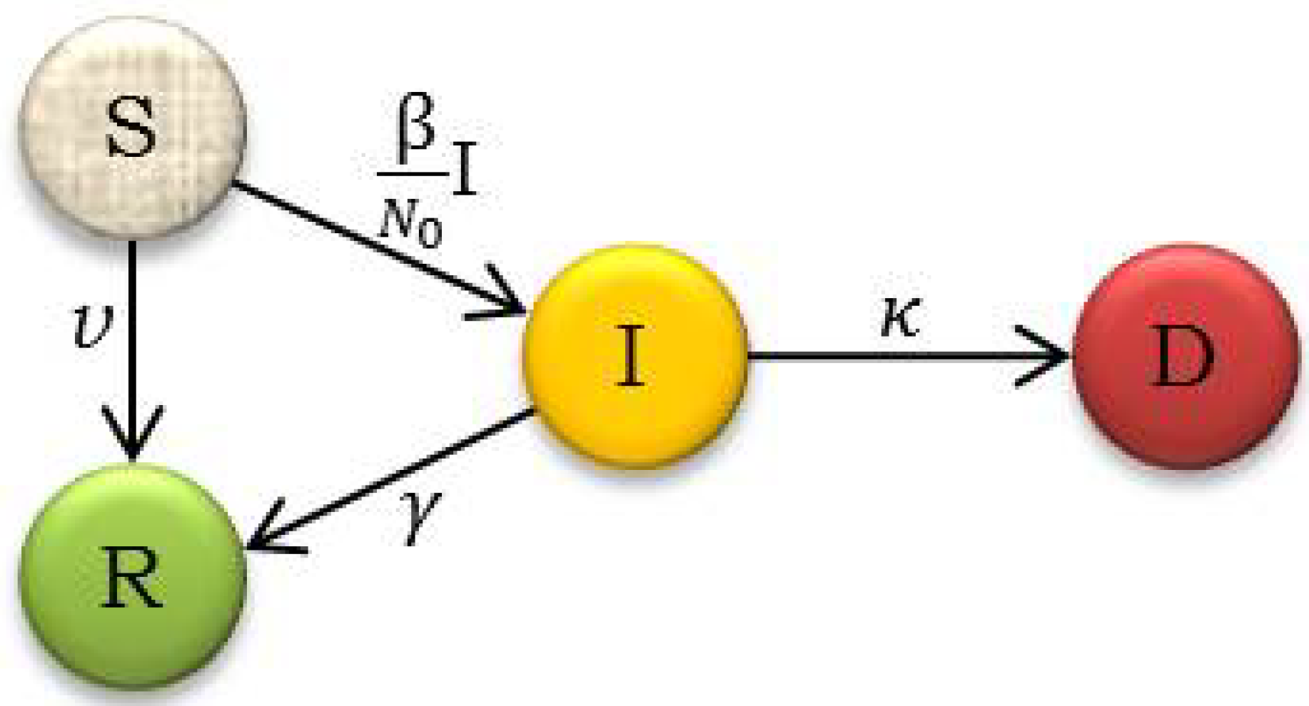
:1. Introduction
- ○
- is the average number of contacts per person per time
- ○
- is the recovery rate,
- ○
- is the death rate.
2. Preliminary and Necessary Definitions
3. Analysis for the Modified SIRD Model of the Pandemic
4. Main Results
- Step 1
- is a nonlinear continuous operator.Let be four positive sequences such that in Then for each we have:where satisfies (12) for each Then, we can find easily that in In fact, we haveSimilarly, we haveSince in we obtainThen, for each we obtain as for anyNow let be such that for each we have:Then, we have:For each the function is integrable Therefore, there exists an implication based on Lebesgue’s dominated convergence theorem and (17), which gives us the following:and hence:Consequently, is continuous.
- Step 2
- Clearly denotes a closed, bounded and convex subset ofThen, in each case, we haveThusor Then Consequently
- Step 3
- is relatively compact.Let and Then, for every we obtainWe have:thenwe have alsoThen (20) givesIt follows from that the right-hand side of the above-mentioned inequality tends to zero,
5. Conclusions
Author Contributions
Funding
Institutional Review Board Statement
Informed Consent Statement
Acknowledgments
Conflicts of Interest
References
- Eitorial Board. Is the World Ready for the Coronavirus? The New York Times, 29 January 2020.
- China virus death toll rises to 41, more than 1300 infected worldwide. CNBC, 24 January 2020.
- Brauer, F.; Castillo-Chavez, C.; Feng, Z. Mathematical Models in Epidemiology; Springer: New York, NY, USA, 2019. [Google Scholar]
- Djordjevic, J.; Silva, C.J.; Torres, D.F.M. A stochastic SICA epidemic model for HIV transmission. Appl. Math. Lett. 2018, 84, 168–175. [Google Scholar] [CrossRef] [Green Version]
- Ndaïrou, F.; Area, I.; Nieto, J.J.; Silva, C.J.; Torres, D.F.M. Mathematical modeling of Zika disease in pregnant women and newborns with microcephaly in Brazil. Math. Methods Appl. Sci. 2018, 41, 8929–8941. [Google Scholar] [CrossRef] [Green Version]
- Rachah, A.; Torres, D.F.M. Dynamics and optimal control of Ebola transmission. Math. Comput. Sci. 2016, 10, 331–342. [Google Scholar] [CrossRef] [Green Version]
- Ullah, A.; Abdeljawad, T.; Ahmad, S.; Shah, K. Study of a fractional-order epidemic model of Childhood diseases. J. Funct. Spaces 2020. [Google Scholar] [CrossRef] [PubMed]
- Samko, S.G.; Kilbas, A.A.; Marichev, O.I. Fractional Integral and Derivatives (Theory and Applications); Gordon and Breach: Lausanne, Switzerland, 1993. [Google Scholar]
- Podlubny, I. Fractional Differential Equations, Mathematics in Science and Engineering; Academic Press: New York, NY, USA, 1999. [Google Scholar]
- Kilbas, A.A.; Srivastava, H.H.; Trujillo, J.J. Theory and Applications of Fractional Differential Equations; Elsevier Science B.V: Amsterdam, The Netherlands, 2006. [Google Scholar]
- Diethelm, K. The Analysis of Fractional Differential Equations; Springer: Berlin, Germany, 2010. [Google Scholar]
- Hasan, A.; Susanto, H.; Tjahjono, V.R.; Kusdiantara, R.; Putri, E.R.M.; Hadisoemarto, P.; Nuraini, N. A new estimation method for COVID-19 time-varying reproduction number using active cases. medRxiv 2020. [Google Scholar] [CrossRef]
- Hilfer, R. Applications of Fractional Calculus in Physics; World Scientific: Singapore, 2000. [Google Scholar]
- Magin, R.L. Fractional Calculus in Bioengineering; Begell House: Danbury, CT, USA, 2006. [Google Scholar]
- Awawdeh, F.; Adawi, A.; Mustafa, Z. Solutions of the SIR models of epidemics using HAM. Chaos Solit. Fract. 2009, 42, 3047–3052. [Google Scholar] [CrossRef]
- Biazar, J. Solution of the epidemic model by Adomian decomposition method. Appl. Math. Comput. 2006, 173, 1101–1106. [Google Scholar] [CrossRef]
- Rafei, M.; Daniali, H.; Ganji, D.D. Variational iteration method for solving the epidemic model and the prey and predator problem. Appl. Math. Comput. 2007, 186, 1701–1709. [Google Scholar] [CrossRef]
- Rafei, M.; Ganji, D.D.; Daniali, H. Solution of the epidemic model by homotopy perturbation method. Appl. Math. Comput. 2007, 187, 1056–1062. [Google Scholar] [CrossRef]
- Almeida, R. Variational problems involving a Caputo-type fractional derivative. J. Optim. Theory Appl. 2017, 174, 276–294. [Google Scholar] [CrossRef]
- Almeida, R.; Malinowska, A.B.; Odzijewicz, T. Fractional differential equations with dependence on the Caputo-Katugampola derivative. J. Comput. Nonlinear Dyn. 2016, 11, 061017. [Google Scholar] [CrossRef] [Green Version]
- Arioua, Y.; Basti, B.; Benhamidouche, N. Initial value problem for nonlinear implicit fractional differential equations with Katugampola derivative. Appl. Math. E-Notes 2019, 19, 397–412. [Google Scholar]
- Basti, B.; Arioua, Y.; Benhamidouche, N. Existence and uniqueness of solutions for nonlinear Katugampola fractional differential equations. J. Math. Appl. 2019, 42, 35–61. [Google Scholar] [CrossRef]
- Basti, B.; Arioua, Y.; Benhamidouche, N. Existence results for nonlinear Katugampola fractional differential equations with an integral condition. Acta Math. Univ. Comen. 2020, 89, 243–260. [Google Scholar]
- Basti, B.; Benhamidouche, N. Existence results of self-similar solutions to the Caputo-type’s space-fractional heat equation. Surv. Maths. Appl. 2020, 15, 153–168. [Google Scholar]
- Basti, B.; Benhamidouche, N. Global existence and blow-up of generalized self-similar solutions to nonlinear degenerate diffusion equation not in divergence form. Appl. Math. E-Notes 2020, 20, 367–387. [Google Scholar]
- Katugampola, U.N. Existence and uniqueness results for a class of generalized fractional differential equations. arXiv 2014, arXiv:1411.5229. [Google Scholar]
- Luchko, Y.; Rivero, M.; Trujillo, J.J.; Velasco, M.P. Fractional models, non-locality and complex systems. Comput. Math. Appl. 2010, 59, 1048–1056. [Google Scholar] [CrossRef] [Green Version]
- Miller, K.S.; Ross, B. An Introduction to the Fractional Calculus and Differential Equations; John Wiley: New York, NY, USA, 1993. [Google Scholar]
- Nisar, K.S.; Ahmad, S.; Ullah, A.; Shah, K.; Alrabaiah, H.; Arfan, M. Mathematical analysis of SIRD model of COVID-19 with Caputo fractional derivative based on real data. Results Phys. 2021, 21, 103772. [Google Scholar] [CrossRef]
- Bagley, R.L.; Torvik, P.J. On the appearance of the fractional derivatives in the behaviour of real materials. J. Appl. Mech. 1984, 51, 294–298. [Google Scholar]
- Katugampola, U.N. A new approach to generalized fractional derivative. Bull. Math. Anal. Appl. 2014, 6, 1–15. [Google Scholar]
- Katugampola, U.N. New approach to a generalized fractional integral. Appl. Math. Comput. 2011, 218, 860–865. [Google Scholar] [CrossRef] [Green Version]
- Nouioua, F.; Basti, B. Global existence and blow-up of generalized self-similar solutions for a space-fractional diffusion equation with mixed conditions. Ann. Univ. Paedagog. Crac. Stud. Math. 2020, 20, 43–56. [Google Scholar]
- Granas, A.; Dugundji, J. Fixed Point Theory; Springer: New York, NY, USA, 2003. [Google Scholar]

Publisher’s Note: MDPI stays neutral with regard to jurisdictional claims in published maps and institutional affiliations. |
© 2021 by the authors. Licensee MDPI, Basel, Switzerland. This article is an open access article distributed under the terms and conditions of the Creative Commons Attribution (CC BY) license (https://creativecommons.org/licenses/by/4.0/).
Share and Cite
Basti, B.; Hammami, N.; Berrabah, I.; Nouioua, F.; Djemiat, R.; Benhamidouche, N. Stability Analysis and Existence of Solutions for a Modified SIRD Model of COVID-19 with Fractional Derivatives. Symmetry 2021, 13, 1431. https://doi.org/10.3390/sym13081431
Basti B, Hammami N, Berrabah I, Nouioua F, Djemiat R, Benhamidouche N. Stability Analysis and Existence of Solutions for a Modified SIRD Model of COVID-19 with Fractional Derivatives. Symmetry. 2021; 13(8):1431. https://doi.org/10.3390/sym13081431
Chicago/Turabian StyleBasti, Bilal, Nacereddine Hammami, Imadeddine Berrabah, Farid Nouioua, Rabah Djemiat, and Noureddine Benhamidouche. 2021. "Stability Analysis and Existence of Solutions for a Modified SIRD Model of COVID-19 with Fractional Derivatives" Symmetry 13, no. 8: 1431. https://doi.org/10.3390/sym13081431