Tachyons and Solitons in Spontaneous Symmetry Breaking in the Frame of Field Theory

Abstract

This paper presents our study of the presence of the unstable critical point in spontaneous symmetry breaking (SSB) in the framework of Ginzburg–Landau (G-L) free energy. Through a 3D Ising spin lattice simulation, we found a zone of hysteresis where the unstable critical point continued to exist, despite the system having entered the broken symmetry phase. Within the hysteresis zone, the presence of the kink–antikink SSB solitons expands and, therefore, these can be observed. In scalar field theories, such as Higgs fields, the mass of this soliton inside the hysteresis zone could behave as a tachyon mass, namely as an imaginary quantity. Due to the fact that groups Ζ(2) and SU(2) belong to the same universality class, one expects that, in future experiments of ultra-relativistic nuclear collisions, in addition to the expected bosons condensations, structures of tachyon fields could appear.

1. Introduction

The most important stage in describing phase transitions within the framework of the theory of critical phenomena is the description and determination of the critical point. The critical point acts as a saddle point in a potential function, while the potential, according to Landau theory, can be described as a polynomial function $U\left(\phi \right)$ of the order parameter $\phi$ [1]. The order parameter $\phi$ describes the Ginzburg–Landau (G-L) free energy and it is invariant under the transform $\phi \to -\phi$:

$$U\left(\phi \right)=\frac{1}{2}{r}_0{\phi }^2+\frac{1}{4}{u}_0{\phi }^4+\frac{1}{6}{c}_0{\phi }^6+\frac{1}{8}{s}_0{\phi }^8+\dots .$$

(1)

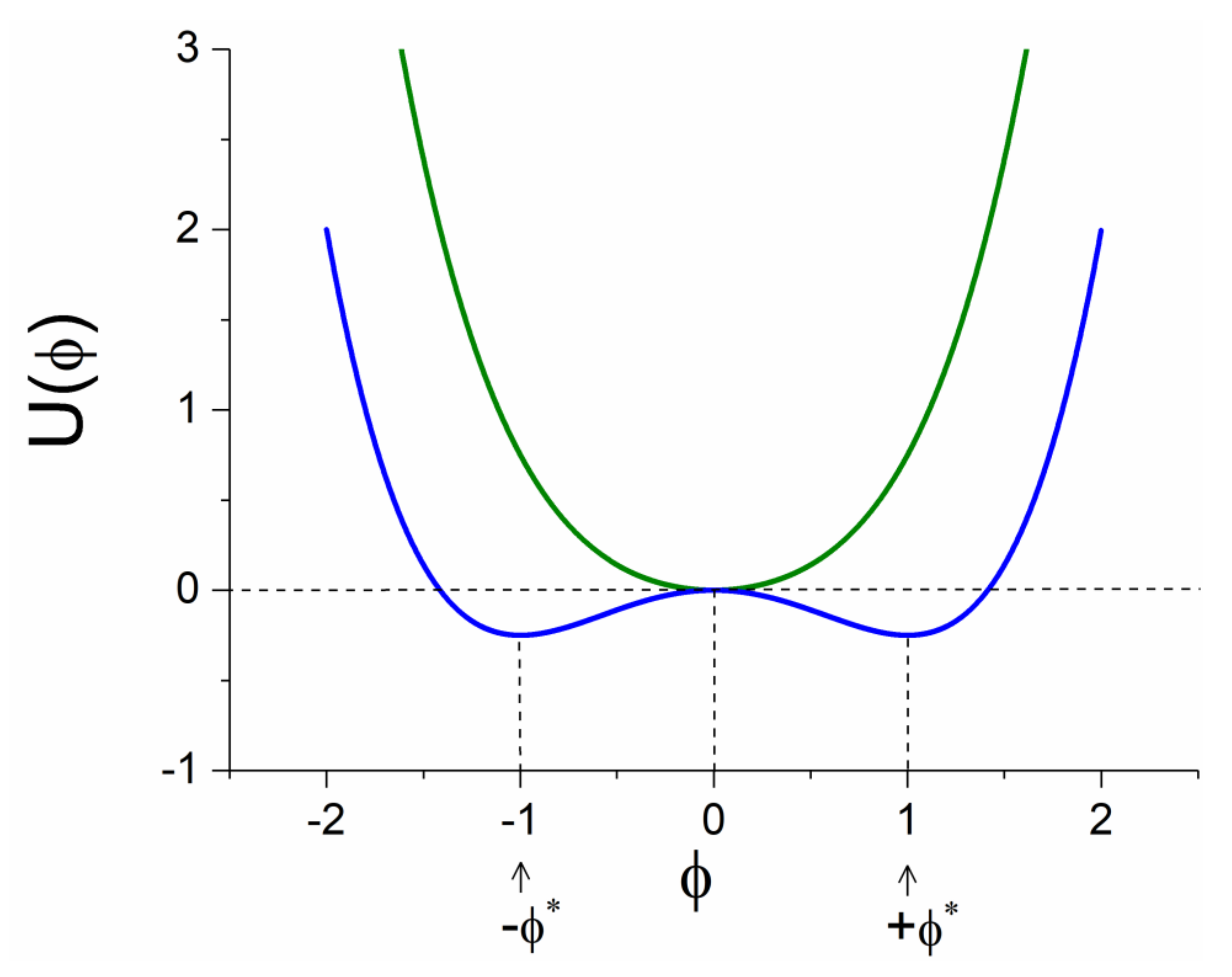
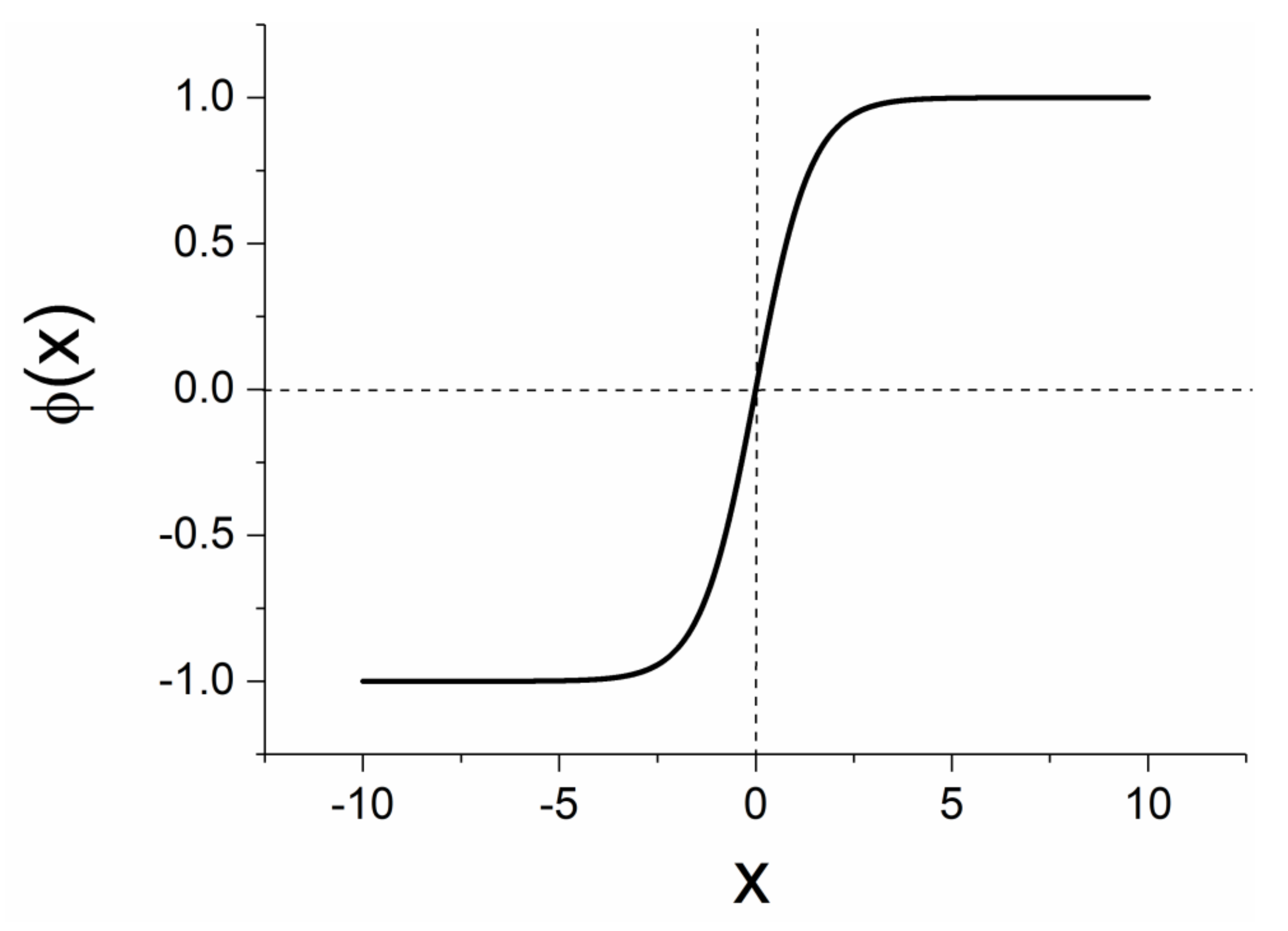
It is noted that, in the symmetric phase, all the coefficients in Equation (1) are positive. This equation can provide a description of the first and second order phase transitions, which can be achieved by utilizing terms up to ${\phi }^6$.

The symmetric phase, in the framework of ${\phi }^4$ theory, is described by the relationship: $U\left(\phi \right)=\frac{1}{2}{r}_0{\phi }^2+\frac{1}{4}{u}_0{\phi }^4$, ($r_0>0, u_0>0)$, illustrated in Figure 1 as the green curve. In this phase, the system exists in the ground state ($\phi =0, U\left(\phi \right)=0).$ The spontaneous symmetry breaking (SSB) [1], achieved for ($r_0<0, u_0>0$), is presented with the blue curve in Figure 1, where the two stable points are the new ground states at the positions ${\phi }^{*}=\pm \sqrt{\frac{r_0}{u_0}}$. The free energy in SSB is:

$$U_{SSB}\left(\phi \right)=-\frac{1}{2}\left|r_0\right|{\phi }^2+\frac{1}{4}{u}_0{\phi }^4, u_0>0.$$

(2)

In nature, the system can exist in only one of these ground states. Thus, the symmetry appears to be broken. An extension to the three dimensions produces the “Mexican hat potential” [2]. When the transition from ($r_0>0, u_0>0)$ to ($r_0<0, u_0>0$) occurs in the G-L free energy parameters, the green curve is converted to the blue one (see Figure 1). The ground state ($\phi =0, U\left(\phi \right)=0)$ in the symmetric phase is the critical stable fixed point for $r_0=0$. When this transition takes place, the position of the critical point does not change, but its character, namely its stability, changes. The stable critical point is converted to an unstable critical point. This change is the most important in critical phenomena because it cancels the existence of a stable critical point at position $\phi =0$ and creates two new degenerated stable fixed points at positions $\pm {\phi }^{*}$. This is necessary for the system to choose one of the two positions and thus the SSB phenomenon is completed.

In field theories, such as the scalar Higgs fields, the parameter $r_0$ can be considered as the $m^2$ quantity, where $m$ is the mass term in the Klein–Gordon wave equation [3]. In fields theories it is common for the parameters $r_0, u_0$ of G-L free energy to be replaced with $r_0\to m^2$ and $u_0\to \lambda$, where $\lambda$ is the coupling parameter of the ${\phi }^4$ self-interaction. Thus, the SSB potential for field theories takes the form:

$$U_{SSB}\left(\phi \right)=\frac{1}{2}{m}^2{\phi }^2+\frac{1}{4}\lambda {\phi }^4, m^2<0, \lambda >0 .$$

(3)

When the system is at the symmetric phase (green curve in Figure 1), $m^2$ is positive. When $m^2$ is negative, the symmetry is broken (blue curve in Figure 1), and the mass is an imaginary quantity. This mass is a tachyon mass [3]. An imaginary mass means that the tachyons move with a speed faster than the speed of light. Since the condition $m^2<0$ is valid for the broken symmetry phase, we conclude that the tachyonic field appears in the phase of the broken symmetry. It is known that the tachyon is a very unstable state [4,5,6,7,8]. As a result, the search for tachyons is connected with the search for instability in the SSB. The only instability that occurs in SSB field theories is the appearance of the unstable critical point when $m^2$ becomes negative. We can therefore conclude that this is the condition for the appearance of tachyons. This means that, with the creation of instability in the G-L ${\phi }^4$ theory, we also have the appearance of tachyons. As soon as the unstable critical point ceases to exist, the tachyon no longer exists.

Topological solitons appear in SSB ${\phi }^4$ theories [2,3]. Is there a connection between these solitons and the tachyons in SSB theories? The connection between tachyons and SSB has been investigated in [4,9] while, in [10], string mass stability is addressed like the stability of mass in SSB. Moreover, the connection between tachyons and bosonic D-brane theory has been made. For example, it has been conjectured that condensation of tachyons on a bosonic D-brane gives rise to vacuum/soliton solutions [11]. In the present work, we investigate whether such a connection between the SSB solitons and the scalar tachyons exists.

Tachyons in nature or in experiments have not yet been detected. This is primarily due to the fact that their highly unstable state excludes the possibility of detection. In this study, we demonstrate that this difficulty can be overcome. Through a numerical experiment with the 3D Ising model, one can follow the evolution of the SSB phenomenon, we found that the unstable state in which the tachyon “lives” can be significantly extended. We suggest that this finding may be used to enable physicists in detecting tachyons. The investigation into the existence of tachyonic fields and SSB solitons for extensive duration is the main purpose of this study.

2. Hysteresis Phenomenon of the Unstable Critical Point in the Broken Symmetry Phase

A question arises: what happens to the evolution of the unstable critical point? It is certain that, as soon as the SSB is completed, the unstable critical point ceases to exist. However, what happens up until that point? The mathematical expression of Equations (2) and (3), as well as its free energy diagram shown in Figure 1 (blue curve), cannot describe the evolution of the unstable critical point. In Figure 1, we can see that the transition to SSB is made immediately by changing the sign of a coefficient. As will be highlighted in the following discussion, this happens at the limit of infinite system length. Therefore, we resort to a numerical experiment with a well-known model that undergoes a second order phase transition: the 3D Ising model. The phase transition in this model is described by the SSB G-L theory [1].

For a Z(N) spin system, spin variables are defined as: $\mathrm{s}\left(a_j\right)=e^{i2\mathsf{\pi }{a}_j/N}$ (lattice vertices $\mathrm{j}=1, 2,\dots j_{max}$), with $a_j=0, 1, 2, 3,\dots N-1$. Specifically, for $N=2$ and for 3 dimensions, we consider the 3D Ising model. An effective algorithm which produces configurations for the 3D Ising model is the metropolis algorithm [12]. In this algorithm, the configurations at constant temperatures are selected with Boltzmann statistical weights $e^{-\beta H}$, where $H$ is the Hamiltonian of the spin system with its nearest neighbors’ interactions, which can be written as:

$$\mathrm{H}=-{{\displaystyle \sum }}_{<k,m>}{J}_{km}{s}_k{s}_m.$$

(4)

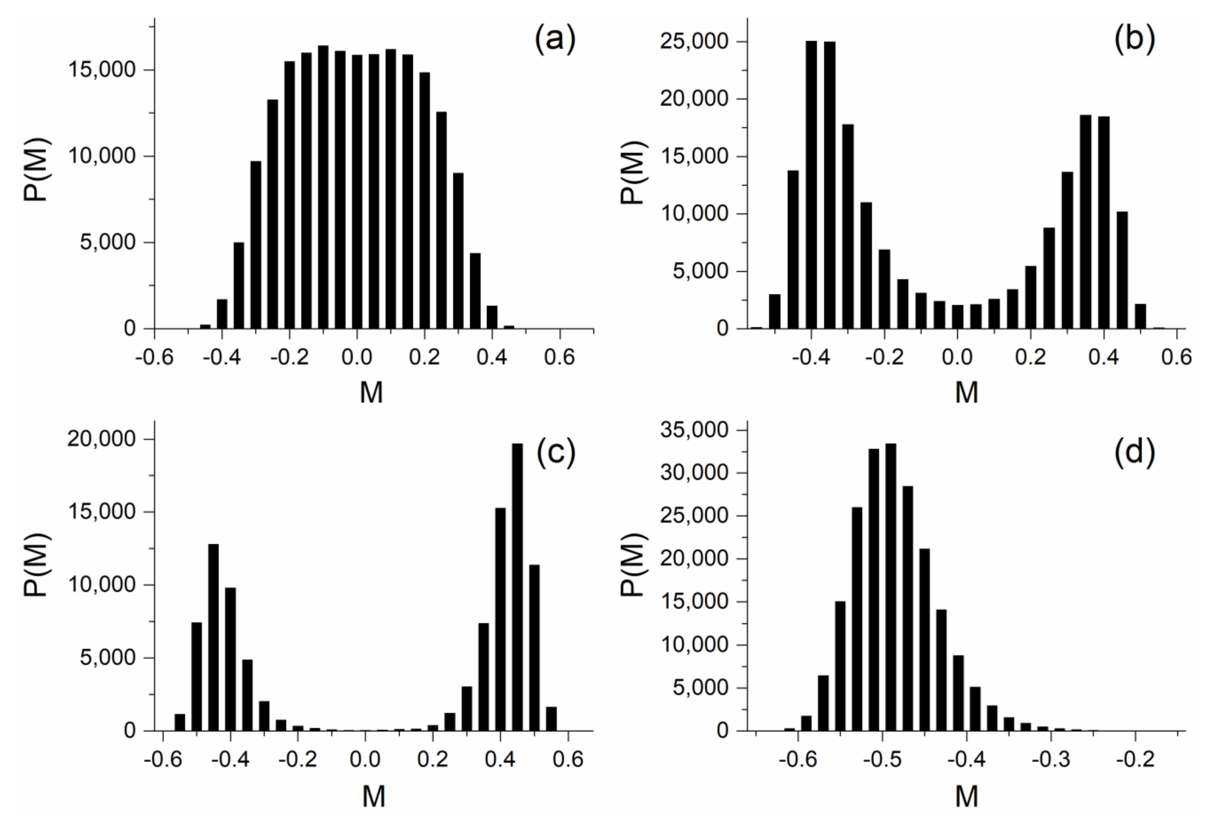
It is known [1] that this model undergoes a second-order phase transition when the temperature falls below a critical (pseudo-critical) value. Thus, for a ${20}^3$ lattice, the critical temperature has been found to be $T_c=4.545$ ($J_{km}=1$) [13]. Therefore, in temperatures lower than this value, an SSB phenomenon appears. The quantity we record in the numerical experiment performed with the metropolis algorithm is the mean magnetization $M$ that plays the role of the order parameter. The trajectory generated by the numerical experiment is a “time series” of the fluctuations of the order parameter. The G-L free energy has the form of Equation (2), with $r_0~\frac{T-T_c}{T_c}$. A time series with length $N_{iter}$ can be recorded with a time-step, the algorithmic time of simulation, which is a lattice sweep. In Figure 2, we present the distribution of the magnetization “time series” for four different temperatures. The simulation was performed for $N_{iter}=200,000$ sweeps. In the limit, where $N_{iter}\to \infty$, the lobes in Figure 2b,c become absolutely symmetrical to each other.

As seen in Figure 2, after the temperature drops under its critical value $T_c$, the new phase of broken symmetry appears, where the “trajectories” of order parameter are attracted by the new ground states. However, for a small temperature interval, the trajectories are not completely separated, but there are trajectories around the critical point. Within this narrow zone of temperatures, the “communication” between the two degenerated vacua is possible due to the existence of the unstable critical point that repels the trajectory from one vacuum to the other. 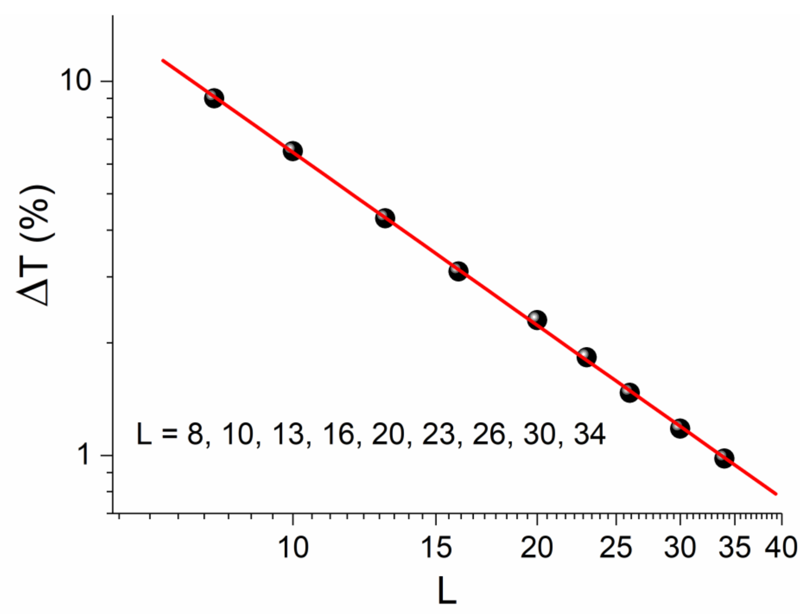Therefore, the unstable critical point does not vanish immediately after the change of sign of the parameter $r_0$ in the G-L free energy of Equation (2), but continues to exist in the phase of broken symmetry. Thus, there is a hysteresis in its disappearance, the width of which depends on the length of the lattice, as shown in Figure 3. We define this hysteresis zone (in the form of percentage) as:

$$\Delta T=\frac{T_c-T_{SSB}}{T_c}·100\%,$$

(5)

where $T_{SSB}$ is the temperature where the lobes no longer “communicate”, and thus, the SSB is completed.

Figure 3 demonstrates a finite size effect at play for the temperature zone in which the unstable critical point survives. As already discussed, the presence of an unstable critical point results in the existence of tachyons in field theories. Thus, in field theories, the life of a tachyon field is not instantaneous, i.e., as soon as we leave the critical value of the control parameter, but instead expands for as long as the hysteresis phenomenon exists. According to this finite size effect, the hysteresis of the unstable critical point is higher in very small spatial distances. Such distances appear in ultra-relativistic experiments in heavy-ion collisions. This issue is further discussed in Section 5.

3. Solitons and Tachyons in SSB

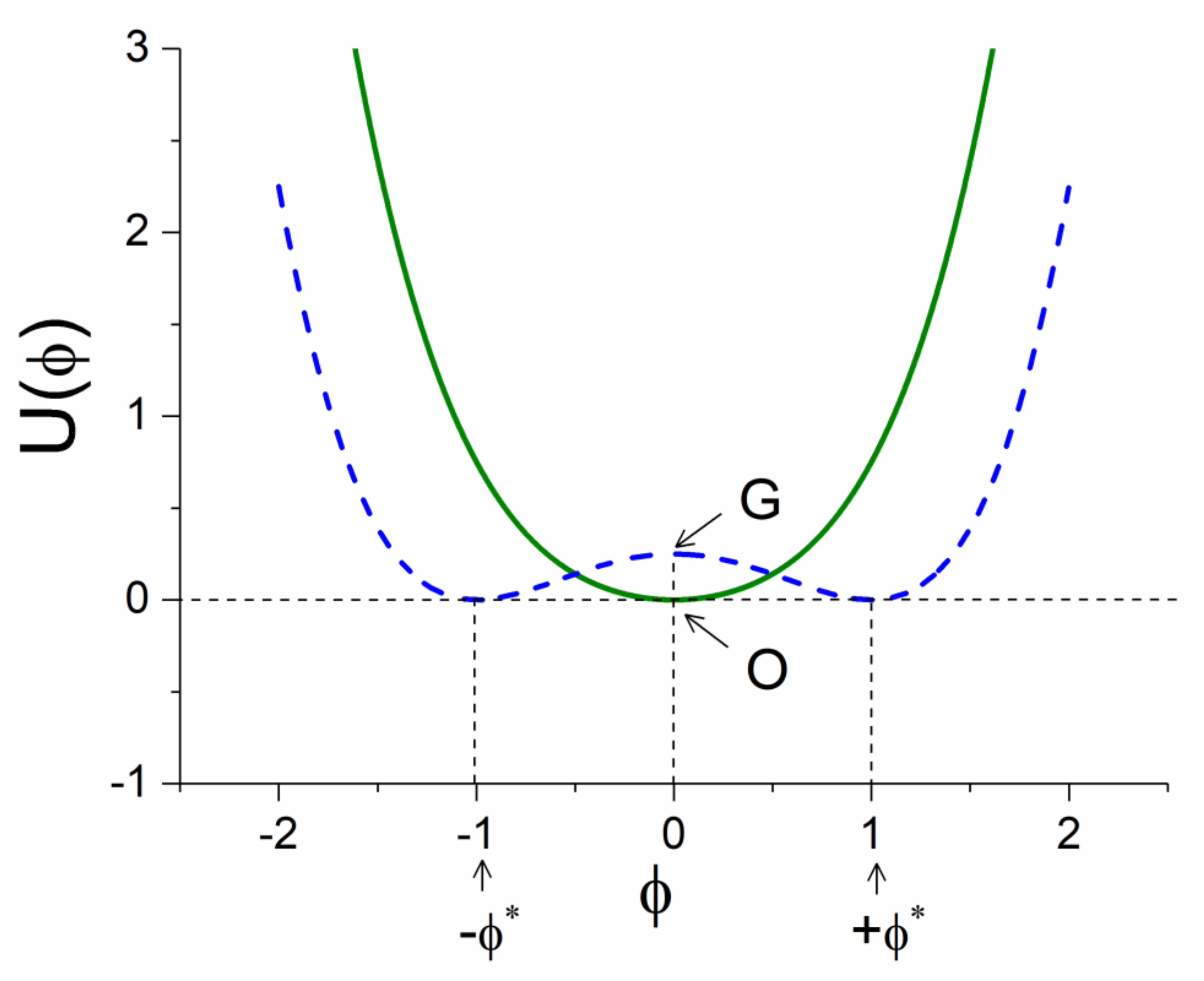
The soliton solution in SSB appears as the critical point is in an excited state G: $\phi =0, U=\frac{r_0{}^2}{4u_0}$ [3], as shown in Figure 4.

The connection between solitons and tachyons has been presented in quantum field theories (QFT) such as String theory [16] and D-branes [17]. An interesting investigation between quantum solitons and tachyons has been attempted in [18]. In QFT, a tachyon is an excitation/particle with negative mass squared. The dynamics of a tachyon in QFT will hence make it form a condensate at a local potential energy minimum.

The classical vacuum is not the same as a quantum vacuum. The quantum vacuum hosts excited states. Therefore, in order for any comparison to be possible, one must excite the ground state of SSB potential by adding the quantity $U=\frac{r_0{}^2}{4u_0}$. Thus, Equation (2) takes the form:

$$U_{SSB}\left(\phi \right)=-\frac{1}{2}\left|r_0\right|{\phi }^2+\frac{1}{4}{u}_0{\phi }^4+\frac{r_0{}^2}{4u_0}, u_0>0.$$

(6)

After this change, the free energies for the symmetrical state and SSB, become as illustrated in Figure 4, where $U_{SSB}$ appears shifted by $U=\frac{r_0{}^2}{4u_0}$ compared to the one presented in Figure 1.

By taking into account Equations (3) and (6) is written in terms of mass as:

$$U_{SSB}\left(\phi \right)=\frac{1}{2}{m}^2{\phi }^2+\frac{1}{4}\lambda {\phi }^4+\frac{m^4}{4\lambda }, m^2<0, \lambda >0,$$

(7)

It is well known from the literature [3] that this potential (Equations (6) and (7)) has soliton solutions of kink and antikink types. In Figure 5 the form of a kink soliton is shown.

According to Equation (7) there is an unstable critical point at position G, shown in Figure 4. In field theory the imaginary mass of tachyons appears when the symmetry is broken. In order for a soliton to present the same behavior as the tachyon, it must also show imaginary mass because it appears in the phase of the broken symmetry. It is known [3] that the mass of SSB soliton for the field theory is given as:

$$M_{soliton}=\frac{2\sqrt{2}}{3\lambda }{m}^3$$

(8)

Equation (8) relates the mass of the particle to the mass of the soliton. As we prove in Section 4, exactly at the point of SSB, the mass of the particle is real; therefore, from Equation (8), it follows that the mass of the soliton is also real. However, when the mass of the particle is tachyonic, which happens while we are in the hysteresis zone due to the fact that the soliton mass $M_{soliton}$ is an odd power of tachyon mass $m$, the mass of the soliton is also imaginary, as long as the hysteresis lasts. Therefore, both tachyon and soliton have the same behavior under the change of the sign of the quantity $m^{2 }$ in the G-L free energy. In other words, they have an imaginary value until the breaking of the symmetry is completed. Exactly on SSB, the tachyon no longer exists and the soliton has real mass.

4. Where Are the Tachyons in the SSB Phase?

If one writes Equation (3) in the form:

$$U_{SSB}\left(\phi \right)=-\frac{1}{2}{\mu }^2{\phi }^2+\frac{1}{4}\lambda {\phi }^4,$$

(9)

where the real mass $\mu$ (${\mu }^2>0$) is connected with the imaginary mass $m$ through the relation $m=i\mu$, then the positions of new vacua are written as:

$${\phi }^{*}=\pm \frac{\mu }{\sqrt{\lambda }} .$$

(10)

Following the standard process for the $U_{SSB}\left(\phi \right)$ estimation inside the new vacua, as in the Higgs scalar field [3], we introduce a new field that perceives the two new vacua as basic states in the theory.

To do this, one needs to take into account the values of ${\phi }^{*}$ in defining the new fluctuation variable, $\eta$, as follows:

$$\eta =\phi \pm \frac{\mu }{\sqrt{\lambda }} .$$

(11)

From Equation (11), by solving for $\phi$, one obtains:

$$\phi =\eta \mp \frac{\mu }{\sqrt{\lambda }} .$$

(12)

By substituting $\phi$ from Equation (12) into Equation (9) (for example, for the ${\phi }_{+}$ case), one obtains:

$$U_{SSB}\left({\phi }_{+}\right)=-\frac{1}{2}{\mu }^2{\phi }^2+\frac{1}{4}\lambda {\phi }^4=-\frac{1}{2}{\mu }^2{\left(\eta +\frac{\mu }{\sqrt{\lambda }}\right)}^2+\frac{1}{4}\lambda {\left(\eta +\frac{\mu }{\sqrt{\lambda }}\right)}^4.$$

(13)

Executing the calculations in Equation (13), we take that:

$$U_{SSB}\left( {\phi }_{+}\right)={\mu }^2{\eta }^2+\mu \sqrt{\lambda }{\eta }^3+\frac{1}{4}\lambda {\eta }^4-\frac{1}{4}\frac{{\mu }^4}{\lambda }.$$

(14)

The following comments can be made regarding Equation (14): (a) the first potential term, which is the mass term for the particle, now has the desirable sign namely the imaginary tachyonic mass is vanished. (b) The second and third terms represent the self-interactions of three and four fields, respectively. (c) The fourth term is a constant quantity, the absolute value of which is the excitation introduced in Equation (7). The ${\eta }^3$ term breaks the symmetry. This is the cost we paid in order to remove the tachyons from the theory, namely we broke the symmetry of the system into field reversal transformations.

In this case, there are no longer tachyon fields in the SSB. However, what happens until the SSB is completed; that is, within the predicted hysteresis zone for finite systems?

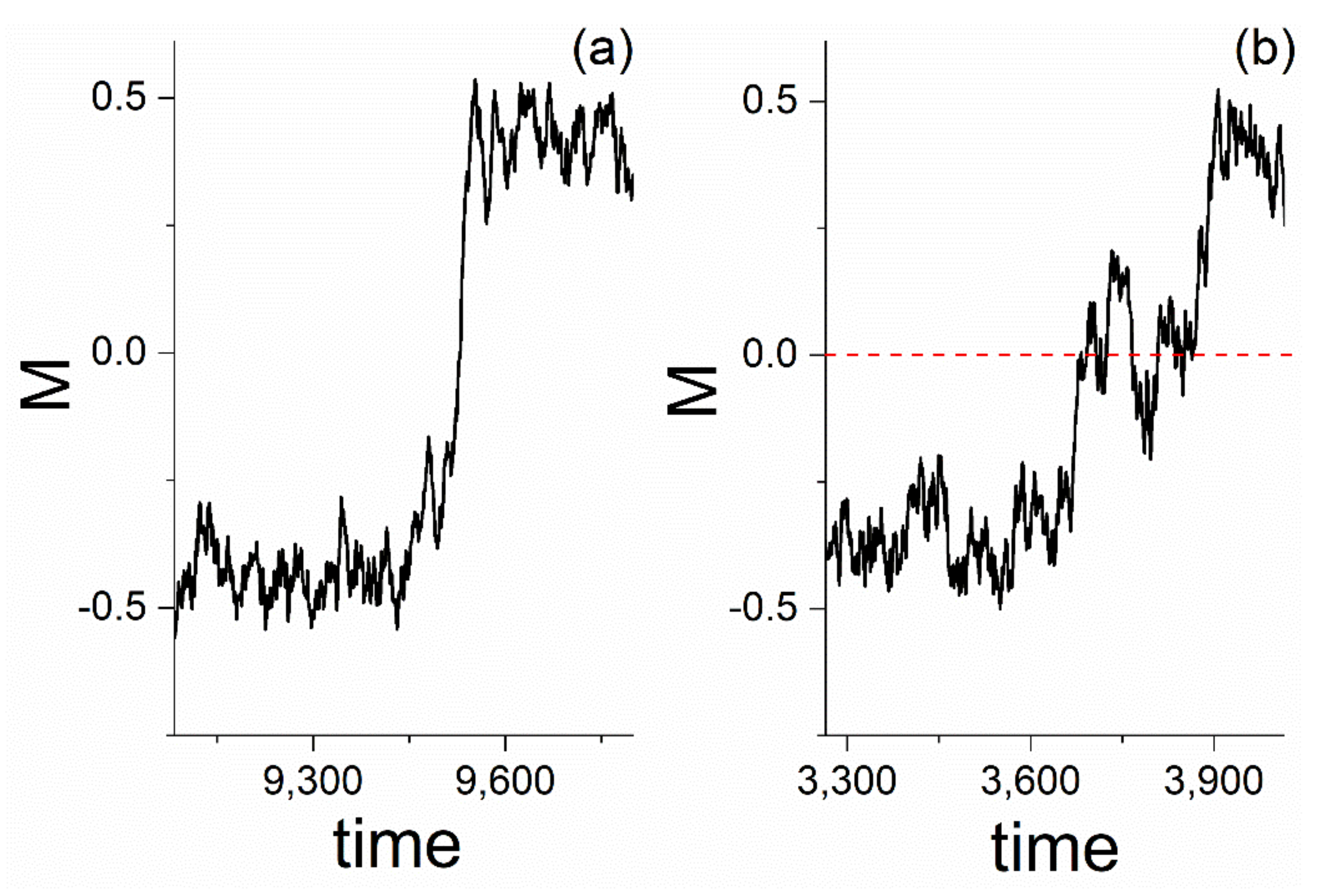
In Figure 6a, a kink-type SSB soliton for a segment of the magnetization time series, just on the SSB (at $T_{SSB}=4.44$), is shown. Figure 6b presents a corresponding segment of the magnetization time series for the temperature $T_{SSB}<\left(T=4.48\right)<T_c$ within the hysteresis zone. The kink–soliton is presented as the transition between the two states $M=\pm 0.5$ (for $N_{iter}\to \infty ).$

In Figure 6a the fluctuations around the new stable vacua appear. In terms of field theory, these are the fluctuations $\eta$ of the Equation (14). These structures do not have tachyonic mass. In Figure 6b fluctuations around the unstable critical point appear as long temperature remains within the hysteresis zone. In terms of quantum field theory, these structures are the interference part resulting from the communication between the vacua inside the hysteresis zone. These fluctuations extend around the unstable critical point and therefore have imaginary mass, i.e., these structures are tachyonic fields.

In an infinite system the hysteresis zone does not exist, which means that the unstable critical point vanishes and, therefore, in the new stable vacua, causality is not violated. Therefore, tachyons are not expected in infinite systems. On the contrary, in finite systems, beyond the expected bosons condensations, tachyon structures such as the ones in Figure 6b would appear until the SSB is completed. The more finite the system, the more possible it is to detect the tachyons.

5. Discussion about Phenomena Within the Zone $\Delta T$

Further detail would shift the scope of this work; therefore, we refer the interested reader to our pre-publication [19] that examines all the important issues concerning the communication of the vacua, the probabilities of the transition between the positive and negative values of magnetization, the scaling behavior within the zone $\Delta T$ and the autocorrelations functions. In this section, we provide only a short introduction to all the above issues.

The tunnelling effect between the two degenerate vacua has been studied in [20], where these are treated as bubbles that are in contact and have developed surface tensions. It would be interesting to prove that the time fluctuations observed in the transition line between the two levels, as in Figure 6b, correspond to the spatial fluctuations of the surface tension that are characterized by local inhomogeneity. On a quantitative level, one could compare the rate of metastable vacuum decay calculated in [20] with the jump probability calculated in [19], where we describe in more detail the hysteresis phenomenon. From the magnetization time series in Figure 6, the probability distribution of the time intervals separating the change of sign of the magnetization from the next could be studied versus $T$ and $L$. This probability has been calculated in [19]. Until the SSB is complete, the domain walls are not yet structures with clear boundaries due to the communication between them, and thus they retain almost all their lengths, small and large. This means that the scaling laws are maintained, as has been proven in [19], the main scope of which was the study of the phenomenon of the hysteresis zone in finite systems. As soon as the symmetry breaking is complete, the domain walls acquire clear boundaries and are completely separated from each other. However, this does not imply that they maintain a constant shape. Their lengths are limited, the scaling laws cease to exist and, thus, there is no longer an unstable critical point. This transformation of the domain walls, expressed through the scaling laws, is another way to see the existence of this $\Delta T$ zone in which the tachyons appear. Finally, a paradox phenomenon occurs where the temporal auto-correlation function is maximized exactly at SSB. The explanation of this phenomenon is presented in [19].

6. Discussion for Tachyons and Solitons at the Critical Point of QCD and Beyond

As mentioned in Section 4, for very small distance, the zone of unstable critical point hysteresis in the broken symmetry phase can “keep in life” the tachyons and kink–antikink solitons. In field theories, we refer to them as spatiotemporal distances. Such very small spatiotemporal distances appear in the ultra-relativistic experiments in heavy-ion collisions. Within the framework of the universality behavior of critical phenomena, the critical behavior of an SU(2) gauge system is analogous to the Ising models which have a global Z(2) spin model symmetry [21,22,23]. The SU(2) gauge symmetry describes in the QCD the confinement-deconfinement phase transition of the bound state $q$-$\overline{q}$. Moreover, it has been shown that QCD phase transition, in ultra-relativistic nuclear collisions, is considered in the framework of the universality class provided by the 3D Ising model [24]. Therefore, it is possible to find in ultra-relativistic nuclear collisions boson field with tachyonic mass, such as the solitons of Figure 6b of the 3D Ising model, within the hysteresis zone.

The search for the tachyonic field near the critical point of QCD has already begun. A recent work investigated the QCD confinement during the tachyon condensation below the critical temperature [25], while [26] investigated the confinement and screening in tachyonic matter, a process much like that of the field of gluons that bind quarks in hadronic matter. Thus, in experiments using very high energy, proximity to the critical point (temperature) of QCD allows for a greater possibility of identifying the unstable critical point in the hadrons matter, according to what we have presented in the present work, and therefore to favor the appearance of tachyon fields. Although critical temperatures are still the subject of research, we consider a good estimate to be 260 Mev for the confinement–deconfinement phase transition and 150 Mev for the chiral phase transition of two flavor [27]. The length $L$ in x-axis of Figure 3 is determined by the ions’ collision energy. As the collision energy increases, the hysteresis zone increases too. Thus, if in an experiment the x-axis of Figure 3 could be calibrated to suitable energy units, then, through the power law of Figure 3, one could deduce the percentage of the hysteresis in order to find the temperature at which the symmetry is actually broken. For example, a spatial size of collisions region which, for Figure 3, corresponds to a $\Delta T=6.5\%,$ would give a hysteresis zone of $6.5\% · 260$ Mev $\approx 17$ Mev, which means that the SSB temperature would appear at 243 Mev. Moreover, focusing on the zone between the $260$ Mev and 243 Mev could reveal, according to what has been presented in this paper, the tachyonic field component expressed by the interference term (Figure 6b). The future experiments that will be carried out in even higher energies, and therefore shorter distances, will be the judge of what we suggest in this work.

According to the present work, as the energy of a collision increases, the hysteresis zone also increases, correspondingly increasing the probability of the observation of tachyons. Thus, the huge energy density of the early universe offers optimal conditions for the existence of tachyons according to what has been presented in the present work. Accordingly, the subject of study of a series of works includes issues such as string tachyons and cosmological collapse [28], quantum theory of solitons [18], string theory of tachyons condensation and universe inflation [29], tachyon matter and cosmology [30], connection of SSB with ultra-light masses in the early universe [31], ultra-light masses and cosmological constant [32].

7. Conclusions—Further Investigations

In the present work, we have found that, in finite systems, the critical temperature does not coincide with the SSB temperature. We have demonstrated that a hysteresis effect occurs in the cease of the unstable state; thus, in field theories, the tachyon can “survive” long enough to be detected. Based on the fact that the mass of SSB soliton is analogous to odd power of the tachyon mass, we conclude that, in field theories, SSB solitons obtain a mass that becomes imaginary, as in the case with tachyons. Moreover, in Z(2) spin models, the solitons are of the type kink–antikink, where the phenomenon of hysteresis increases the presence of solitons so that they can be observed. The fluctuations around the $M=0$ in kink–antikink structures is the signature of the appearance of tachyons. Due to the fact that the groups Ζ(2) and SU(2) belong to the same universality class, in future experiments of ultra-relativistic nuclear collisions within the defined hysteresis zone, one expects the appearance of the tachyonic field component. Thus, beyond the expected condensation of bosons, the tachyonic field could also be recorded, which violates the causality. In order to overcome the problem of causality, one could repeat the study in another space where the problem of causality does not exist. Such a space is the Euclidean space. In a recent work [33], the phase space of SSB was studied. Specifically, it was found that, under some special conditions, very strong instability in the position of the critical point in Euclidean time appeared [33]. This finding offers indirect indications towards the existence of tachyons without facing the problematic causality issue, since Euclidean time is the inverse temperature. Therefore, one can study the tachyons field according to the described method in Section 4, if transferred to the momentum space of high energy experiments. This is a worthwhile field for future research.