
Research Risk Factors in Monitoring Well Drilling—A Case Study Using Machine Learning Methods

 ,
, 
 ,
,
Abstract
:1. Introduction
2. Existing Methodologies
2.1. Logistic Regression
2.2. Naive Bayesian Classifier
2.3. Method K-Nearest Neighbors
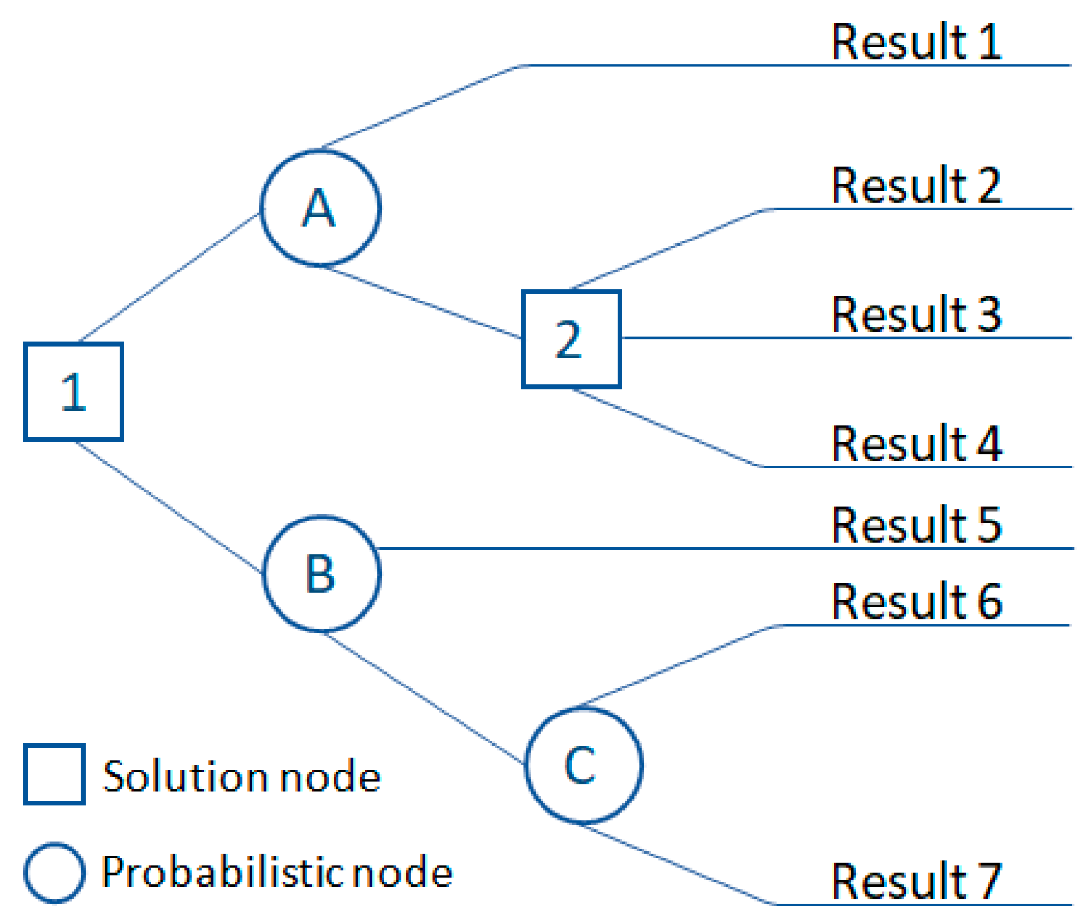
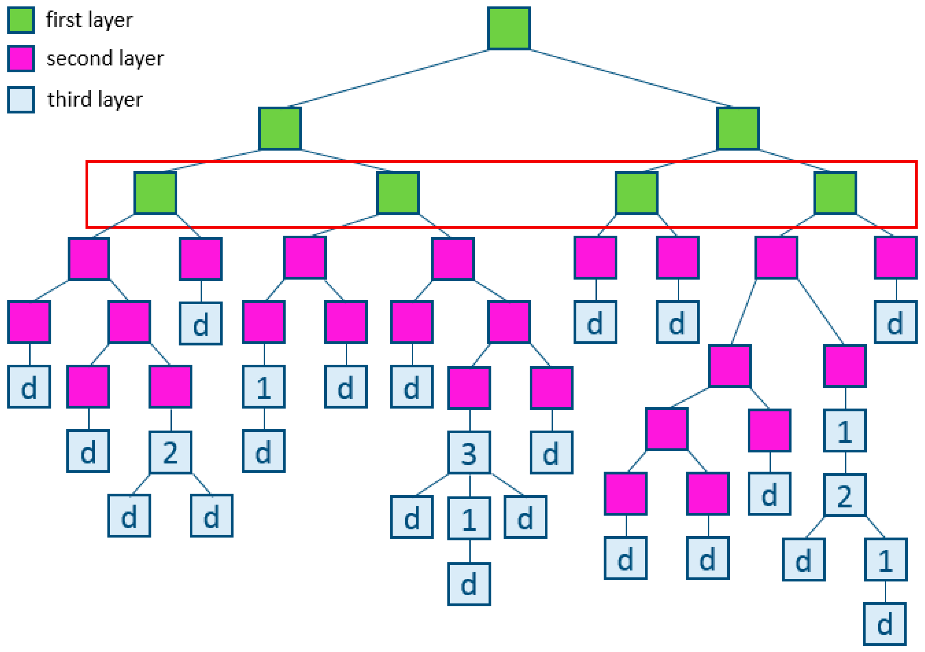
2.4. Decision Tree
- Decision node: This is often represented by squares that show what can be conducted. The lines coming out of the square show all the available options available on the node.
- Probability knot: This is often represented by circles showing random results. Exodus odds are events that can occur but are beyond the control of the manager.
- Closing node: This is represented by triangles or lines that do not have additional solution nodes or random nodes. Terminal nodes represent the final outcomes of the decision process.
2.5. Support Vector Machine
2.6. Random Forest
2.7. Gradient Boosting
2.8. Neural Network
2.9. Evaluation of the Quality of Machine Learning Methods
2.10. Precision, Recall, and F-Score
3. Given Data
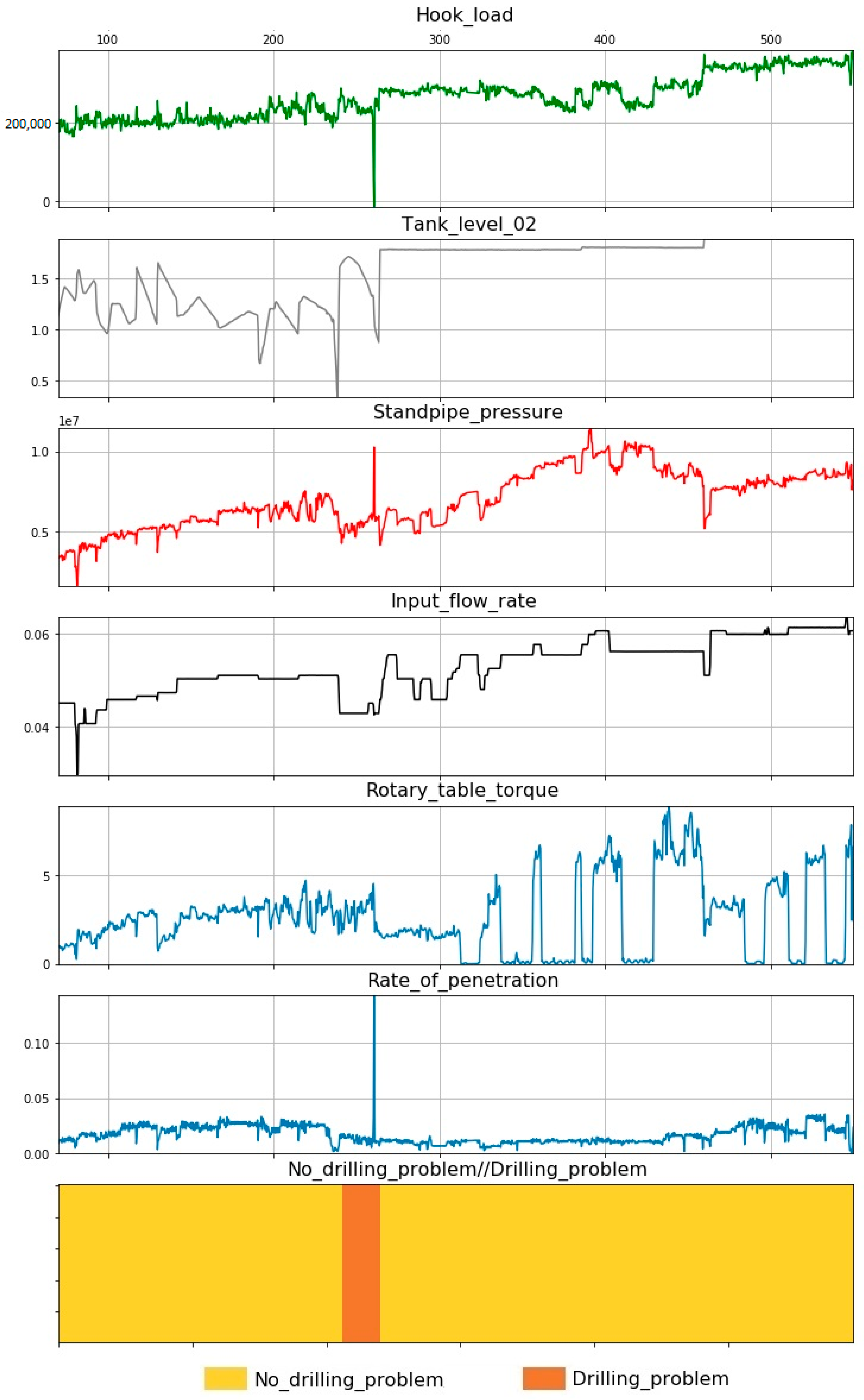
4. Results
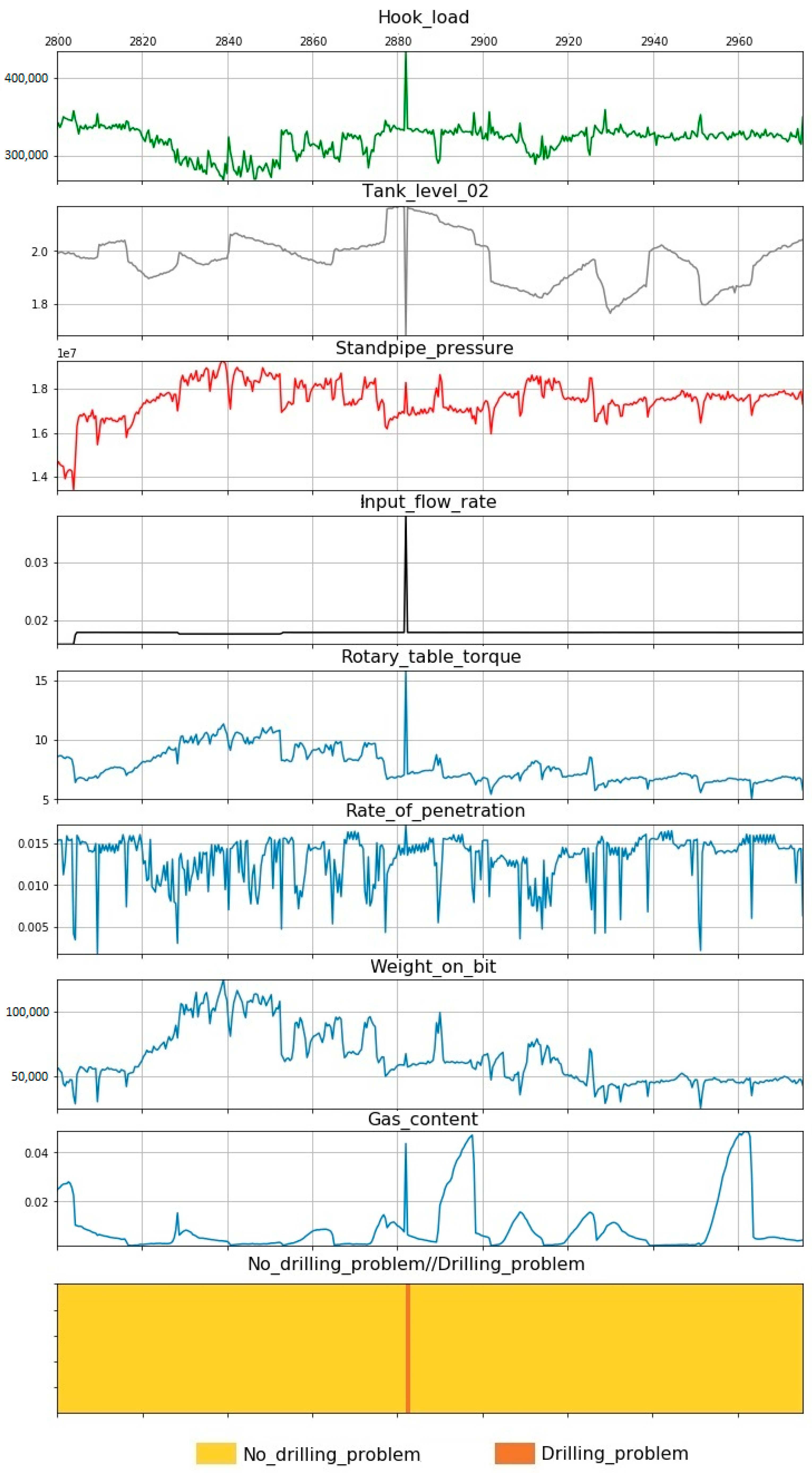
- Standpipe pressure;
- Tank level 02;
- Input flow rate;
- Hook load;
- Rotary table torque;
- Rate of penetration;
- Weight on bit;
- Gas content.
5. Discussion
6. Conclusions
- Based on the literature review, a wide application of AI in drilling was shown, from the creation of training programs to the prediction of the rate of penetration.
- During the analysis of the initial data, wells with problems that were encountered during drilling were identified. To model the presented DPs, a computer model was set up.
- During the analysis of the drilling reports, a list of the main parameters was compiled, which participated as input for the model: standpipe pressure; tank level; input flow rate; hook load; rotary table torque; rate of penetration; weight on bit; gas content.
- Of the eight methods of machine learning (ML), the GB method was chosen. This algorithm showed a high-performance precision, recall, and F-score.
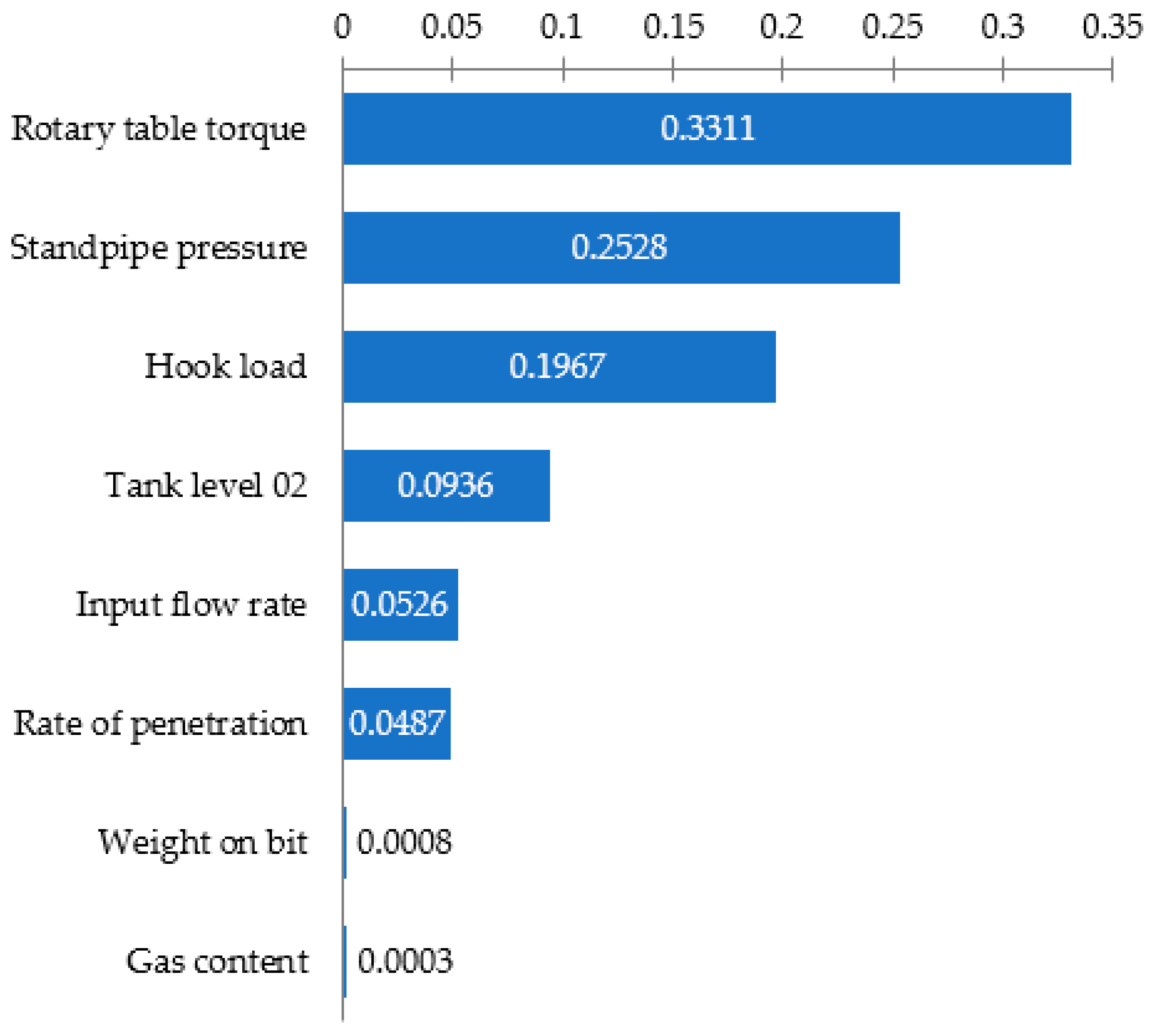
- For the GB method, the parameters that make the greatest contribution to the operation of the algorithm were established using the feature importation parameter. These are the rotary table torque, standpipe pressure, and hook load.
- During the GB analysis, it was established that in the case of removing parameters such as gas content, the model continued to work without changing the accuracy of the classification of the DPs.
- Although the ultimate goal of this work was to teach the program to classify the problems in the drilling process, in the future, it is necessary to consider the possibility of predicting the drilling problems in real time, for example, using time series. Such a model will avoid problems, preventing high costs.
- In the future, it is necessary to train the algorithm on a larger number of data on wells with problems. This will expand the application of the program and elucidate how to classify various types of drilling problems.
- It will be useful to test the model by specifying not only drilling parameters but also geophysical logging data, on the input. This will allow models to take into account such a parameter as lithology. Depending on the different rocks, the log data will show the different behaviors of the curves.
- It is also recommended to use geomechanical parameters of the formation as input data. These data will allow predicting possible problem areas of the well in advance that are prone to collapse.
Author Contributions
Funding
Institutional Review Board Statement
Informed Consent Statement
Data Availability Statement
Conflicts of Interest
Abbreviations
| AI | Artificial intelligence |
| DPs | Drilling problems |
| GB | Gradient boosting |
| ML | Machine learning |
| PID | Proportional–integral–differential |
| ROP | Process rate of penetration |
| RSS | Rotary steerable system |
References
- Hochreiter, S.; Schmidhuber, J. Long short-term memory. Neural Comput. 1997, 9, 1735–1780. [Google Scholar] [CrossRef] [PubMed]
- Jones, D.T. Protein secondary structure prediction based on position-specific scoring matrices. J. Mol. Biol. 1999, 292, 195–202. [Google Scholar] [CrossRef] [Green Version]
- LeCun, Y.; Bengio, Y.; Hinton, G. Deep learning. Nature 2015, 521, 436–444. [Google Scholar] [CrossRef]
- Milo, R.; Shen-Orr, S.S.; Itzkovitz, S.; Kashtan, N.; Chklovskii, D.M.; Alon, U. Network motifs: Simple building blocks of complex networks. Science 2002, 298, 824–827. [Google Scholar] [CrossRef] [Green Version]
- Nielsen, H.; Engelbrecht, J.; Brunak, S.; Heijne, G.V. Identification of prokaryotic and eukaryotic signal peptides and prediction of their cleavage sites. Protein Eng. 1997, 10, 1–6. [Google Scholar] [CrossRef] [Green Version]
- Olden, J.D.; Jackson, D.A. Illuminating the “black box”: A randomization approach for understanding variable contributions in artificial neural networks. Ecol. Model. 2002, 154, 135–150. [Google Scholar] [CrossRef]
- Reichstein, M.; Camps-Valls, G.; Stevens, B.; Jung, M.; Denzler, J.; Carvalhais, N. Deep learning and process understanding for data-driven Earth system science. Nature 2019, 566, 195–204. [Google Scholar] [CrossRef]
- Rubinov, M.; Sporns, O. Complex network measures of brain connectivity: Uses and interpretations. NeuroImage 2010, 52, 1059–1069. [Google Scholar] [CrossRef] [PubMed]
- Tu, J.V. Advantages and disadvantages of using artificial neural networks versus logistic regression for predicting medical outcomes. J. Clin. Epidemiol. 1996, 49, 1225–1231. [Google Scholar] [CrossRef]
- Voyant, C.; Notton, G.; Kalogirou, S.; Nivet, M.-L.; Paoli, C.; Motte, F.; Fouilloy, A. Machine learning methods for solar radiation forecasting: A review. Renew. Engergy 2017, 105, 569–582. [Google Scholar] [CrossRef]
- Almeida, T.L.P.; Passos, B.A.F.; Costa, J.L.S.; Andrade, A.J.N. Identifying clay mineral using angular competitive neural network: A machine learning application for porosity estimative. J. Pet. Sci. Eng. 2021, 200, 108303. [Google Scholar] [CrossRef]
- Hajizadeh, Y. Machine learning in oil and gas; a SWOT analysis approach. J. Pet. Sci. Eng. 2019, 176, 661–663. [Google Scholar] [CrossRef]
- Hanga, K.M.; Kovalchuk, Y. Machine learning and multi-agent systems in oil and gas industry applications: A survey. Comput. Sci. Rev. 2019, 34, 100191. [Google Scholar] [CrossRef]
- Nima, M.; Hamzeh, G.; David, A.W.; Mohammad, M.; Shadfar, D.; Sina, R.; Alireza, S.; Amirafzal, K.S. A geomechanical approach to casing collapse prediction in oil and gas wells aided by machine learning. J. Pet. Sci. Eng. 2021, 196, 107811. [Google Scholar]
- Mohamed, L.; Mohamed, S.; Sofiène, T. Detection and sizing of metal-loss defects in oil and gas pipelines using pattern-adapted wavelets and machine learning. Appl. Soft Comput. 2017, 52, 247–261. [Google Scholar]
- Sina, R.; Mohammad, M.; Hamzeh, G.; David, A.W.; Nima, M.; Jamshid, M.; Shadfar, D. Determination of bubble point pressure & oil formation volume factor of crude oils applying multiple hidden layers extreme learning machine algorithms. J. Pet. Sci. Eng. 2021, 202, 108425. [Google Scholar]
- Hao, C.; Chao, Z.; Ninghong, J.; Ian, D.; Shenglai, Y.; Yong, Z.Y. A machine learning model for predicting the minimum miscibility pressure of CO2 and crude oil system based on a support vector machine algorithm approach. Fuel 2021, 290, 120048. [Google Scholar]
- Boikov, A.V.; Savelev, R.V.; Payor, V.A.; Potapov, A.V. Evaluation of bulk material behavior control method in technological units using dem. CIS Iron Steel Rev. 2020, 20, 3–6. [Google Scholar] [CrossRef]
- Litvinenko, V.S.; Tsvetkov, P.S.; Molodtsov, K.V. The social and market mechanism of sustainable development of public companies in the mineral resource sector. Eurasian Min. 2020, 2020, 36–41. [Google Scholar] [CrossRef]
- Kamatov, K.A.; Buslaev, G.V. Solutions for drilling efficiency improvement in extreme geological conditions of Timano-Pechora region. In Proceedings of the SPE Russian Petroleum Technology Conference, Moscow, Russia, 26 October 2015; pp. 1–10. [Google Scholar]
- Charfeddine, L.; Barkat, K. Short-and long-run asymmetric effect of oil prices and oil and gas revenues on the real GDP and economic diversification in oil-dependent economy. Energy Econ. 2020, 86, 104680. [Google Scholar] [CrossRef]
- Aleksandrova, T.; Aleksandrov, A.; Nikolaeva, N. An investigation of the possibility of extraction of metals from heavy oil. Miner. Process. Extr. Metall. Rev. 2017, 38, 92–95. [Google Scholar] [CrossRef]
- Nevskaya, M.A.; Seleznev, S.G.; Masloboev, V.A.; Klyuchnikova, E.M.; Makarov, D.V. Environmental and business challenges presented by mining and mineral processing waste in the Russian Federation. Minerals 2019, 7, 445. [Google Scholar] [CrossRef] [Green Version]
- Liu, T.; Leusheva, E.; Morenov, V.; Li, L.; Jiang, G.; Fang, C.; Zhang, L.; Zheng, S.; Yu, Y. Influence of polymer reagents in the drilling fluids on the efficiency of deviated and horizontal wells drilling. Energies 2020, 13, 4704. [Google Scholar] [CrossRef]
- Gang, H.; Zhaoqiang, X.; Guorong, W.; Bin, Z.; Yubing, L.; Ye, L. Forecasting energy consumption of long-distance oil products pipeline based on improved fruit fly optimization algorithm and support vector regression. Energy 2021, 224, 120153. [Google Scholar]
- Yurak, V.V.; Dushin, A.V.; Mochalova, L.A. Vs sustainable development: Scenarios for the future. J. Min. Inst. 2020, 242, 242–247. [Google Scholar] [CrossRef]
- Kondrasheva, N.K.; Rudko, V.A.; Kondrashev, D.O.; Gabdulkhakov, R.R.; Derkunskii, I.O.; Konoplin, R.R. Effect of delayed coking pressure on the yield and quality of middle and heavy distillates used as components of environmentally friendly marine fuels. Energy Fuels 2019, 33, 636–644. [Google Scholar] [CrossRef]
- Kondrasheva, N.K.; Rudko, V.A.; Ancheyta, J. thermogravimetric determination of the kinetics of petroleum needle coke formation by decantoil thermolysis. ACS Omega 2020, 5, 29570–29576. [Google Scholar] [CrossRef] [PubMed]
- Seçkin, K.; Aytaç, A.; Stelios, B.; Wasim, A. A new forecasting model with wrapper-based feature selection approach using multi-objective optimization technique for chaotic crude oil time series. Energy 2020, 212, 118750. [Google Scholar]
- Hebert, D.; Misiti, A. The Growing Role of Artificial Intelligence in Oil and Gas. Available online: https://insights.globalspec.com/article/2772/the-growing-role-of-artificial-intelligence-in-oil-and-gas (accessed on 23 April 2021).
- Zhan, S.; Rodiek, J.; Heuermann-Kuehn, L.E.; Baumann, J. Prognostics health management for a directional drilling system. In Proceedings of the Prognostics and System Health Management Conference, Shenzhen, China, 24–25 May 2011; pp. 1–7. [Google Scholar]
- Wang, Y. Drilling Hydraulics Optimization Using Neural Networks; University of Louisiana at Lafayette Press: Lafayette, LA, USA, 2015. [Google Scholar]
- Camci, F.; Chinnam, R.B. Dynamic bayesian networks for machine diagnostics: Hierarchical hidden Markov models vs. competitive learning. In Proceedings of the International Joint Conference on Neural Networks, Montreal, QC, Canada, 31 July–4 August 2005; pp. 1–6. [Google Scholar]
- Yang, Z.R.; Yang, Z. Comprehensive Biomedical Physics, 1st ed.; Elsevier Science & Technology: Stockholm, Sweden, 2004. [Google Scholar]
- Lind, Y.B.; Kabirova, A.R. Artificial neural networks in drilling troubles prediction. In Proceedings of the SPE Russian Oil and Gas Exploration & Production Technical Conference and Exhibition, Moscow, Russia, 14–16 October 2014; pp. 1–7. [Google Scholar]
- Al-yami, A.S.H.; Schubert, J. Systems and Methods for Expert Systems for Well Completion using Bayesian Decision Models (BDNs), Drilling Fluids Types, and Well Types. Available online: https://hdl.handle.net/1969.1/177120 (accessed on 23 April 2021).
- Jahanbakhshi, R.; Keshavarzi, R.; Jafarnezhad, A. Real-time prediction of rate of penetration during drilling operation in oil and gas wells. In Proceedings of the Rock Mechanics/Geomechanics Symposium, Chicago, IL, USA, 24–27 June 2012; pp. 1–9. [Google Scholar]
- Monazami, M.; Hashemi, A.; Shahbazian, M. Drilling rate of penetration prediction using artificial neural network: A case study of one of Iranian southern oil fields. J. Oil. Gas. Bus. 2012, 6, 21–31. [Google Scholar]
- Amer, M.M.; Dahab, A.S.; El-Sayed, A.H. An ROP predictive model in nile delta area using artificial neural networks. In Proceedings of the SPE Kingdom of Saudi Arabia Annual Technical Symposium and Exhibition, Dammam, Saudi Arabia, 24–27 April 2017; pp. 1–11. [Google Scholar]
- Gidh, Y.; Purwanto, A.; Bits, S. Artificial neural network drilling parameter optimization system improves ROP by predicting/managing bit wear. In Proceedings of the SPE Intelligent Energy International, Utrecht, The Netherlands, 27–29 March 2012; pp. 1–13. [Google Scholar]
- Rashidi, B.; Hareland, G.; Nygaard, R. Real-time drill bit wear prediction by combining rock energy and drilling strength concepts. In Proceedings of the Abu Dhabi International Petroleum Exhibition and Conference, Abu Dhabi, United Arab Emirates, 3–6 November 2008; pp. 1–9. [Google Scholar]
- Valisevich, A.; Ruzhnikov, A.; Bebeshko, I.; Moreno, R.; Zhentichka, M.; Bits, S. Drillbit optimization system: Real-time approach to enhance rate of penetration and bit wear monitoring. In Proceedings of the SPE Russian Petroleum Technology Conference, Moscow, Russia, 26–28 October 2015; pp. 1–14. [Google Scholar]
- Dashevskiy, D.; Dubinsky, V.; Macpherson, J.D. Application of neural networks for predictive control in drilling dynamics. In Proceedings of the SPE Annual Technical Conference and Exhibition, Houston, TX, USA, 3–6 October 1999; pp. 1–9. [Google Scholar]
- GirirajKumar, S.M.; Jayaraj, D.; Kishan, A.R. PSO based tuning of a PID controller for a high-performance drilling machine. Int. J. Comput. Appl. 2010, 1, 12–18. [Google Scholar] [CrossRef]
- Lind, Y.B.; Samsykin, A.V.; Galeev, S.R. Information and analytical system for prevention of drilling fluid loss. In Proceedings of the SPE Russian Petroleum Technology Conference, Moscow, Russia, 26–28 October 2015; pp. 1–12. [Google Scholar]
- Hegde, C.; Wallace, S.; Gray, K. Real Time prediction and classification of torque and drag during drilling using statistical learning methods. In Proceedings of the SPE Eastern Regional Meeting, Morgantown, VA, USA, 13–15 October 2015; pp. 1–13. [Google Scholar]
- Okpo, E.E.; Dosunmu, A.; Odagme, B.S. Artificial neural network model for predicting wellbore instability. In Proceedings of the SPE Nigeria Annual International Conference and Exhibition, Lagos, Nigeria, 2–4 August 2016; pp. 1–10. [Google Scholar]
- Unrau, S.; Torrione, P.; Hibbard, M.; Smith, R.; Olesen, L.; Watson, J. Machine learning algorithms applied to detection of well control events. In Proceedings of the SPE Kingdom of Saudi Arabia Annual Technical Symposium and Exhibition, Dammam, Saudi Arabia, 24–27 April 2017; pp. 1–10. [Google Scholar]
- Shchepetov, O.A. System classification of failures in drilling. Vestn. Astrakhan State Tech. Univ. Ser. Manag. Comput. Sci. Inform. 2009, 2, 36–42. [Google Scholar]
- Aldred, W.; Plumb, D.; Bradford, I.; Cook, J.; Gholkar, V.; Cousins, L.; Minton, R.; Fuller, J.; Goraya, S.; Tucker, D. Managing drilling risk. Oilfield Rev. 1999, 11, 2–19. [Google Scholar]
- Dvoynikov, M.V. Research on technical and technological parameters of inclined drilling. J. Min. Inst. 2017, 223, 86–92. [Google Scholar]
- Litvinenko, V.S.; Dvoynikov, M.V. Methodology for determining the parameters of drilling mode for directional straight sections of well using screw downhole motors. J. Min. Inst. 2020, 41, 105–112. [Google Scholar] [CrossRef]
- Logistical Regression for Kettles: Detailed Explanation. Available online: https://www.machinelearningmastery.ru/logistic-regression-for-dummies-a-detailed-explanation-9597f76edf46/ (accessed on 2 July 2021).
- Vorontsov, K.V. Lectures on Linear Classification Algorithms; Moscow Institute of Physics and Technology Press: Moscow, Russia, 2009. [Google Scholar]
- Commonly Used Machine Learning Algorithms (with Python and R Codes). Available online: https://www.analyticsvidhya.com/blog/2017/09/common-machine-learning-algorithms/ (accessed on 2 July 2021).
- Ray, S. Easy Steps to Learn Naive Bayes Algorithm with Codes in Python and R. Available online: https://www.analyticsvidhya.com/blog/2017/09/naive-bayes-explained/ (accessed on 23 April 2021).
- Piryonesi, S.M.; Tamer, E.E. Role of data analytics in infrastructure asset management: Overcoming data size and quality problems. J. Transp. Eng. Part B Pavements 2020, 146, 1–7. [Google Scholar] [CrossRef]
- Decision Tree Classifier. Available online: http://mines.humanoriented.com/classes/2010/fall/csci568/portfolio_exports/lguo/decisionTree.html (accessed on 2 July 2021).
- Vorontsov, K.V. Lectures on the Support Vector Machine; Moscow Institute of Physics and Technology Press: Moscow, Russia, 2007. [Google Scholar]
- Chistyakov, S.P. Random forest. Proc. Karelian Res. Cent. Russ. Acad. Sci. 2013, 1, 117–136. [Google Scholar]
- Vorontsov, K.V. Mathematical Methods of Learning by Precedents: A Course of Lectures; Moscow Institute of Physics and Technology Press: Moscow, Russia, 2009. [Google Scholar]
- Matthew, M. More Steps to Mastering Machine Learning with Python. Available online: http://www.kdnuggets.com/2017/03/seven-more-steps-machine-learning-python.html (accessed on 23 April 2021).
- McCulloch, U.S.; Pitts, V. Logical Calculus of Ideas Relating to Nervous Activity; Foreign Literature Publishing House: Moscow, Russia, 1956. [Google Scholar]
- Labintcev, E. Metrics in the Problems of Machine Learning. Available online: https://habrahabr.ru/company/ods/blog/328372/ (accessed on 23 April 2021).
- Nelson, A. Driving Efficiency in the Oil and Gas Industry. Available online: https://biarri.com/driving-efficiency-oil-gas-industry/ (accessed on 23 April 2021).
- Nybø, R. Efficient Drilling Problem Detection; Norwegian University of Science and Technology Press: Trondheim, Norway, 2009. [Google Scholar]
- Nybø, R.; Sui, D. Closing the integration gap for the next generation of drilling decision support systems. In Proceedings of the SPE Intelligent Energy Conference & Exhibition, Utrecht, The Netherlands, 1–3 April 2014; pp. 1–10. [Google Scholar]


| y = 1 | y = 0 | |
|---|---|---|
| y’ = 1 | True Positive (TP) | False Positive (FP) |
| y’ = 0 | False Negative (FN) | True Negative (TN) |
| Algorithm | Metrics (Determination of Drilling Problems) | ||
|---|---|---|---|
| Precision | Recall | F-Score | |
| Logistic regression | 0.00 | 0.00 | 0.00 |
| Naive Bayesian classifier | 0.03 | 1.00 | 0.06 |
| Method of k-nearest neighbors | 0.83 | 0.64 | 0.73 |
| Decision tree | 0.97 | 0.87 | 0.92 |
| Support vector method | 0.00 | 0.00 | 0.00 |
| Random forest | 0.98 | 0.93 | 0.95 |
| Gradient boosting | 1.00 | 0.93 | 0.97 |
| Neural network | 1.00 | 0.53 | 0.70 |
| Algorithm | Situation | Right | False |
|---|---|---|---|
| Logistic regression | Normal | 3916 | 1 |
| Naive Bayesian classifier | Normal | 2484 | 1433 |
| Method of k-nearest neighbors | Normal | 3911 | 6 |
| Decision tree | Normal | 3916 | 1 |
| Support vector method | Normal | 3917 | 0 |
| Random forest | Normal | 3915 | 2 |
| Gradient boosting | Normal | 3917 | 0 |
| Neural network | Normal | 3917 | 0 |
| Algorithm | Situation | Right | False |
|---|---|---|---|
| Logistic regression | Problem | 0 | 45 |
| Naive Bayesian classifier | Problem | 45 | 0 |
| Method of k-nearest neighbors | Problem | 29 | 16 |
| Decision tree | Problem | 39 | 6 |
| Support vector method | Problem | 0 | 45 |
| Random forest | Problem | 39 | 6 |
| Gradient boosting | Problem | 42 | 3 |
| Neural network | Problem | 27 | 18 |
Publisher’s Note: MDPI stays neutral with regard to jurisdictional claims in published maps and institutional affiliations. |
© 2021 by the authors. Licensee MDPI, Basel, Switzerland. This article is an open access article distributed under the terms and conditions of the Creative Commons Attribution (CC BY) license (https://creativecommons.org/licenses/by/4.0/).
Share and Cite
Islamov, S.; Grigoriev, A.; Beloglazov, I.; Savchenkov, S.; Gudmestad, O.T. Research Risk Factors in Monitoring Well Drilling—A Case Study Using Machine Learning Methods. Symmetry 2021, 13, 1293. https://doi.org/10.3390/sym13071293
Islamov S, Grigoriev A, Beloglazov I, Savchenkov S, Gudmestad OT. Research Risk Factors in Monitoring Well Drilling—A Case Study Using Machine Learning Methods. Symmetry. 2021; 13(7):1293. https://doi.org/10.3390/sym13071293
Chicago/Turabian StyleIslamov, Shamil, Alexey Grigoriev, Ilia Beloglazov, Sergey Savchenkov, and Ove Tobias Gudmestad. 2021. "Research Risk Factors in Monitoring Well Drilling—A Case Study Using Machine Learning Methods" Symmetry 13, no. 7: 1293. https://doi.org/10.3390/sym13071293