Particle-Based Dynamic Water Drops with High Surface Tension in Real Time

Abstract

Surface tension has a great influence on the shape of the fluid interface, and is an important physical characteristic in expressing not only liquids but also liquid metals such as mercury and gallium. In the field of physics-based particle fluid simulations, it is a challenging problem to express the high surface tension generated by fluid-air or fluid-solid interaction in real time. The main reasons for this are (1) The magnitude of the force that can be stably expressed in real-time fluid simulation is limited, so when the magnitude of the surface tension increases at a large time-step, the simulation stability decreases, and (2) If we use a small time-step, a stronger force can be expressed. However, it becomes difficult to operate in real time because the computational cost increases. Techniques were proposed to solve this problem for a few specific scenes, but there has not yet been a general approach that can reliably express high surface tension in various scenarios. In this paper, we propose a real-time particle-based fluid simulation framework that can efficiently and stably express high surface tension. Unlike the previous methods, we newly model the surface tension so that the strong surface tension force generated in the droplet area with a large curvature is applied evenly in the normal and tangent directions regardless of the size of the droplet. We also propose new pressure constraints that converge quickly and accurately using this force. Our method can be effectively used in various physics-based simulation scenarios because it can easily express and control surface tension effects that appear in materials such as liquid metal as well as water.

1. Introduction

Fluid dynamics plays an important role in various fields such as visual effects (VFX) [1,2], games [3,4], forensic investigation [5], and weather prediction/analysis [6,7]. Particle-based fluids techniques such as MPM (Material Point Method) [8,9], FLIP (Fluid-Implict Particle) [10,11,12], APIC (Affine Particle-In-Cell) [13,14], Polynomial PIC [15], and SPH (Smoothed Particle Hydrodynamics) [16,17,18] are useful in creating splashes and expressing free surfaces in detail, so they have been widely used in computer graphics in recent years.

Small-scale thin features, such as water streamlets and liquid sheets, are presented in an interesting shape in physics-based liquid simulation. However, their details are often lost due to the resolution limit and numerical instability, and preventing this problem is one of the challenging problems in simulation. To address this problem, various approaches have been introduced in grid-based Eulerian simulation [19,20,21,22] and mesh-based Lagrangian simulation [23,24,25,26,27], but not much of the solution has been presented for SPH simulation. SPH is used in many applications due to its efficiency and flexibility in handling mass preservation or topological changes. However, since SPH is sensitive to the number of particles constituting the feature to be expressed, it becomes more difficult to express small-scale thin features when the number of particles around the liquid surface is insufficient in free surface flow.

In the SPH-based fluid simulation system, challenging problems for various effects that occur when expressing surface tension have been defined and solutions have been proposed. Unlike recent studies on the resolution limit of particle-based simulation [28,29,30,31], this study focuses on modeling pressure constraints that can stably express multiscale surface tension in real-time particle-based fluids. Methods of modeling surface tension based on particle-based fluids are broadly classified as follows: (1) A method of transmitting curvature calculated from particles to external forces, (2) A method to solve the surface tension problem at the molecular level using cohesion forces between adjacent fluid particles, (3) A method using modified SPH formulation [32], and (4) A method of transmitting mesh-based curvature as external force [33]. However, most of them focused on expressing the surface tension in a particular scene. With these techniques, particle clustering occurs near the free surface when handling large surface tension, and momentum cannot be preserved while minimizing surface curvature. In this paper, we present an algorithm that can stably express the surface tension of various intensities that can occur in general scenes.

It is difficult to interactively express not only the low surface tension of liquid metal but also the high surface tension of droplets on a wide leaf using the existing particle-based surface tension technique. The intensity of surface tension depends on the contact angles between the ground and the droplet (see Figure 1). The simulation becomes numerically unstable when attempting to represent a large surface tension in interactive SPH with a high time-step. If the size of the allowable external force is increased using a small time-step, the computational cost increases in inverse proportion to the size of the time-step, which is far from interactive performance. We propose two methods to allow the large surface tension to be interactively expressed in SPH: (1) The surface tension is newly modeled so that the strong surface tension forces generated in the droplet area with large curvature can be applied evenly regardless of the size of the droplet, (2) Pressure constraints are modeled to stably represent multiscale surface tension in particle-based fluids.

Problem Statement

Akinci et al. proposed a multiscale surface tension to change a large curvature to a small size using the particle-based normal vector gradient as a surface tension [34]. In this study, spherical droplets on a small scale were represented by reducing the size of the entire curvature. However, geometrically, when the curvature of a specific area decreases, the curvature of other areas increases, so the curvature cannot completely converge to zero. In particle-based fluids, a curvature smaller than $\frac{1}{r}(\mathrm{where} r \mathrm{is} \mathrm{radius})$ cannot be expressed, so the force to reduce curvature continues to act even on an already spherical droplet. In large droplets with small curvature, the surface tension force is small, so the numerical problem is not very noticeable, but in small droplets with large curvature, the force increases and the movement of particles becomes unstable (see Figure 2).

In most cases, excessive force is generated only in the large curvature area, so even if the difference in curvature is used, a process of evenly distributing the force is required. We model a method of evenly distributing the force according to the relative direction of the normal vector and the relative position of the particle, therefore stably expressing the surface tension even in the large curvature area. To express a strong force, a numerically stable method is most often used. PBD (Position Based Dynamics) [35] expresses physics-based simulation quickly and stably by applying position-based constraints to various fields such as fluid, rigid-body, deformable body, hair, and rope [18,36,37,38,39]. PBF (Position Based Fluids) [18] used PBD as a pressure solver for particle-based fluids, and additional forces such as surface tension were solved through external forces. PBF can stably express a larger external force than previous techniques, but the force was smaller than the force applied as constraints. Therefore, we improved the pressure constraints of PBF so that the larger force than when the surface tension was applied as an external force could be expressed stably. As a result, we designed the pressure force to stably express the surface tension by inducing the direction in which the pressure converges toward the direction in which the surface tension is applied.

When trying to represent adjacent droplets, in the existing SPH technique, the physical quantities of adjacent free surfaces are dissipated by the smoothing kernel, so they are merged into one. It can be expressed by making the radius of the kernel smaller, but the amount of computation increases. Moreover, even if the radius of the kernel becomes smaller, it cannot prevent other droplets from entering the kernel. It is possible to preserve the physical quantities of the free surfaces by classifying droplets into multiple phases, but updating the phase for each droplet is a very tedious and computationally intensive problem in a dynamic scene where the droplets continuously merge and split. To solve this problem, we modeled a simple method that can classify the phase of the adjacent particle according to the region containing it. We differentiated the area of the particle by comparing the normal direction of the water particle, and expressed it as if it were contained in the region of another phase. As a result, it is possible to express separate droplets by preventing the particles from being immediately merged in the adjacent free surface area.

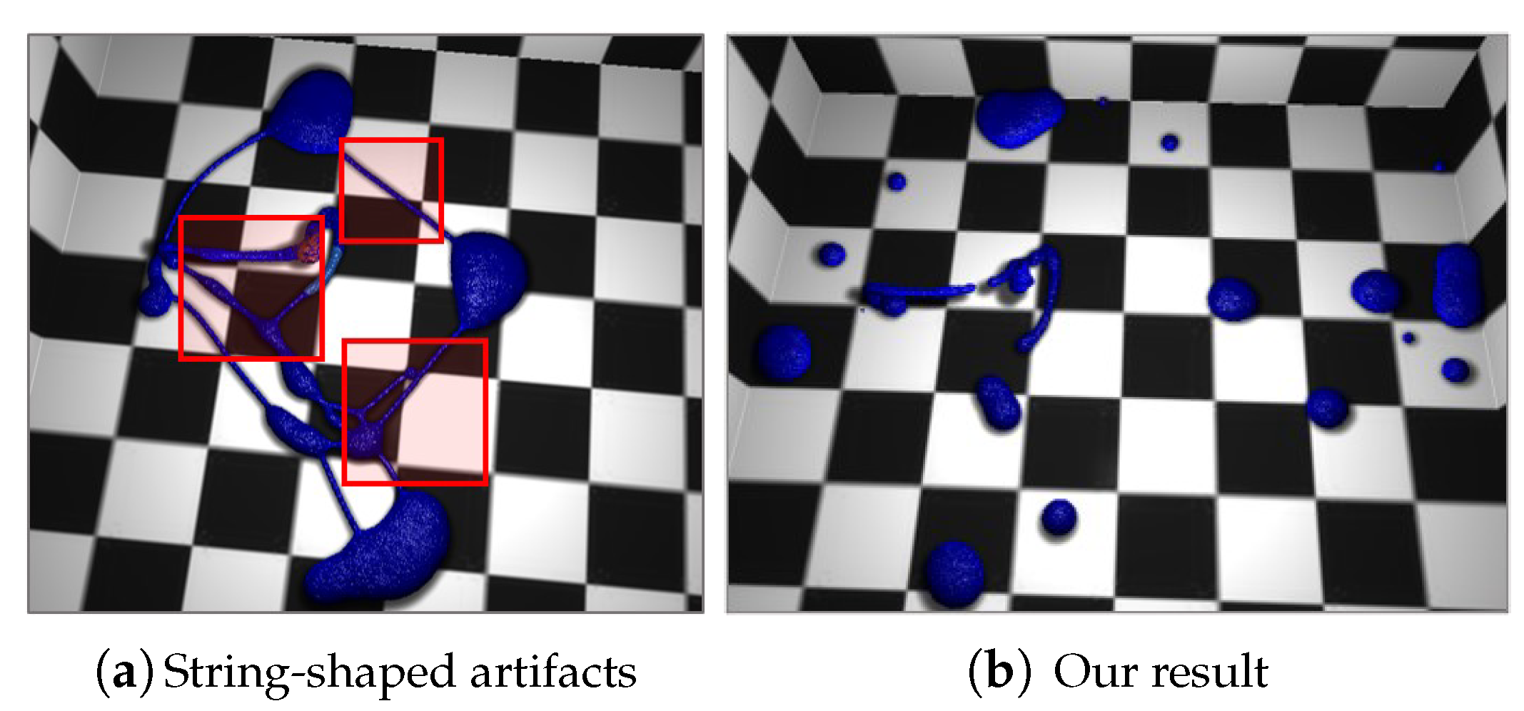
Several different forces were modeled to create an interactive and stable SPH system. A typical example is a method of applying artificial pressure to keep particles at a constant distance without clumping together. However, it sometimes shows artifacts in which string shapes appear (see Figure 3). This string shape occurs when the artificial pressure to maintain a constant distance between particles and the pressure force to resist the force coexist in the separated fluid region. Due to these artifacts, it is expressed as if the viscosity of the fluid is strong, and especially when applied with surface tension, it often shows an odd appearance due to the coexistence of droplets and string shapes (see Figure 3). String shape regions were detected by calculating their orientation and stretch through covariance calculated based on the distribution of water particles. We control the force to maintain the string shape by continuously reducing the pressure force that causes the artifacts according to the size of the string shape, therefore expressing droplets without artifacts.

In this study, the surface tension is newly modeled so that the forces can be applied evenly regardless of the size of the droplet, and we propose pressure constraints that can stably express the multiscale surface tension.

2. Related Work

Various approaches were proposed to calculate the surface tension in SPH simulation. In the early days, methods to express the surface tension with a smoothed color field were mainly proposed [16,40,41,42]. The color function models proposed by Morris [40] and Müller et al. [16] are the basic models widely used when expressing surface tension in particle-based fluids. This method has been applied in earnest to the surface tension model by Becker and Teschner [17] and Adams et al. [28]. This approach evolved into a scalar field-based approach in which the location of the particle is set to 1 and the rest area is set to 0. This approach allows the calculation of surface tension forces by calculating surface normal vectors and curvatures. However, in this approach, the normal vectors of the particles far from the surface are calculated randomly, resulting in incorrect motion. This problem not only causes errors in the curvature values, but also does not guarantee the conservation of fluid momentum.

Surface tension model is usually expressed in macroscopic and microscopic perspectives in SPH fluids [43]. Macroscopic models are called CSF (Continuum Surface Force) models [44] and express surface tension using the color field calculated at the interface of two phases (i.e., fluid and air) [16,40,44,45]. The force is expressed perpendicular to the interface of two phases to obtain a smaller curvature value [44,45,46]. The color field is normalized so that tension forces act between multiple liquids instead of free surfaces [46]. The microscopic model considers the cohesion between particles based on the attractive forces between molecules [17,47,48]. Hu and Adams improved the robustness over the CSF method by formulating the surface tension with the divergence of the stress tensor rather than the surface normal [49]. Sirotkin and Yoh proposed a new smoothing kernel and gradient correction terms to avoid compressional instability that occurs in the CSF method [50]. Particle-based surface tension flow can be calculated using IIF (Inter-particle Interaction Force) as shown by Nugent and Posch [47]. Tartakovsky and Meakin simulated surface tension and fluid-solid coupling effects using the IIF method [48]. Becker and Teschner used the IIF method to calculate the surface tension at free surface flows [17].

The accuracy of CSF and IIF greatly depends on the number of particles used, and the higher the number of particles, the higher it is. Especially for thin features, using a small number of particles increases artifacts and noise noticeably. As an alternative, Zhang et al. [26,51] proposed reconstruction of liquid surfaces to calculate surface tension, and Yu et al. [33] expressed the liquid surfaces as triangular meshes to calculate the surface tension force. Both methods are more effective than particle-based surface tension calculation methods, but are not suitable for use in real-time or interactive applications because of the large amount of additional calculations. Schechter and Bridson created ghost particles on the air side of free surfaces to improve performance [52]. However, this method increases the amount of computation as the scene becomes more complex, and when the scene contains many thin features, the computational overhead required to process ghost particles is large.

In the field of nanofluids, Yaghub and Jamalabadi proposed a technique to express magnetohydrodynamic and nanoparticle effects [53]. However, it is not suitable to extend the multiscale surface tensions algorithm based on the SPH framework proposed in our method. Recently, Far et al. proposed a soluble surfactants simulation technique using the multiphase-based Lattice Boltzmann technique [54], and Daneshfaraz et al. proposed a novel downstream system capable of moving water from high altitudes to lower levels [55]. However, these methods are also difficult to express multiscale surface tensions.

3. Proposed Framework

To express the multiscale surface tension, we improved the instability of the existing technique that occurs in a large curvature so that a larger surface tension can be expressed. In addition, the phase was classified using the normal vector of adjacent particles, and separated nearby droplets that were difficult to express with the existing technique were expressed. In addition, string-shaped artifacts are automatically found and controlled so that the surface tension is expressed in a natural form. The proposed technique solves the following subproblems:

• Improving instability of surface tension force calculated in large curvature area.
• Iterative pressure solver with surface tension.
• Phase classification of droplets using normal vector of adjacent particles.
• Controlling the string-shaped artifact using a particle covariance matrix.

3.1. Surface Tension

The surface tension observed in natural phenomena is determined by the intermolecular force to minimize the contact area with other surfaces. However, since it is difficult to accurately simulate the intermolecular force in SPH, the force that minimizes curvature in the smallest particle unit is generally modeled. Müller et al. [16] calculated the curvature of the surface using the laplacian of the smoothed color field, and determined the direction of the force by calculating the gradient of the smoothed color field. However, this method lacks stability because curvature must be calculated directly and two differentiations are performed on the color field. In addition, it is applied to the particles in a non-symmetric way, so the momentum is not preserved. To solve this problem, Akinci et al. [34] directly applied the difference between the normal vectors of particles to the surface tension, and modeled the symmetric force that minimizes the surface as follows (see Equations (1) and (2)).

$${\mathbf{n}}_i=h\sum _j\frac{m_j}{{\rho }_j}\nabla W\left(\left|{\mathbf{x}}_{ij}\right|\right)$$

(1)

$${\mathbf{f}}_{ij}^s=-\gamma m_i\left({\mathbf{n}}_i-{\mathbf{n}}_j\right)K_{ij}$$

(2)

where i and j are neighboring fluid particles, m is the mass of particle, $\mathbf{x}$ is its position (and ${\mathbf{x}}_{ij}={\mathbf{x}}_i-{\mathbf{x}}_j$), $\rho$ the density and, W is smoothing SPH kernel function with kernel radius h. $\mathbf{n}$ is normal field vector of the particle. $\gamma$ is a positive surface tension coefficient, and the larger the value, the higher the surface tension. ${\mathbf{f}}_{ij}^s$ is the surface tension force on particle i from particle j. $K_{ij}$ is a symmetrized correction factor equal to the value of $\frac{2{\rho }_0}{{\rho }_i+{\rho }_j}$ where ${\rho }_0$ is the rest density.

As shown in the above equation, it can be seen that the surface tension force is modeled in the direction to converge the curvature to zero by reducing the difference between the direction and size of the normal vectors of the adjacent particles. Surface tension is a phenomenon to minimize curvature of fluid, but curvature of droplets cannot converge below $\frac{1}{r}$, where r is the minimum radius of a spherical droplet that a particle can make. According to the above equation, even if the droplets converge into a perfect sphere, the force to reduce the curvature of the droplets is continuously generated. In particular, in small droplets, the minimum curvature is large, so a large force is generated, which decreases the stability of the simulation. In particular, we improved the problem by reducing the magnitude of the force generated by the small droplets.

From Equations (1) and (2), it can be seen that the magnitude and direction of the force is determined by the difference in the normal vector of the particles. In Figure 4a, the normal vector of adjacent particles in a small curvature area shows a larger difference in direction than in size. We simulated the force applied to the particles according to the curvature change in order to find out the effect of this small curvature direction difference on the size of the surface tension. As shown in Figure 4b, assuming that the particles are perfectly circular droplets, the position of the droplets on the surface is continuously changed according to the angle, and the average and instantaneous magnitude of the force are expressed in a graph. In the case of using the existing technique, it can be seen that a large force acts in a region with a large curvature (see Figure 5), and the force deviation caused by the difference in the direction of the normal vector is large (see Figure 6). We modeled the surface tension that can reduce the force deviation caused by the direction of the normal vector as follows (see Equation (3)).

$${\mathbf{f}}_{ij}^s=-\gamma m_i〈{\widehat{\mathbf{n}}}_i·{\widehat{\mathbf{n}}}_j〉\left({\mathbf{n}}_i-{\mathbf{n}}_j\right)K_{ij}$$

(3)

where $\widehat{\mathbf{n}}$ is the unit vector of $\mathbf{n}$. The $〈{\widehat{\mathbf{n}}}_i·{\widehat{\mathbf{n}}}_j〉$ term reduces excessive interference due to the difference in normal vector direction between adjacent particles in a small curvature area. $〈x〉:=\frac{x+\left|x\right|}{2}$ are Macaulay brackets that take only positive values. This makes it possible to more stably express the surface tension by reducing the interference caused by the normal vector in the opposite direction when expressing droplets smaller than h. Comparing this modeled force with the previous technique, it can be seen that the large force seen in a small area is relatively weakened (see Figure 5 and Figure 6).

3.2. Novel Constraints of Surface Tension

In particle-based fluids, forces such as pressure force due to particle density, viscosity force due to the difference in velocity between particles, and surface tension due to curvature act simultaneously. However, it is difficult to satisfy all the convergence conditions of forces, so it is generally designed to prioritize the convergence of important conditions: In general, incompressibility and divergence-free conditions are first solved iteratively, and other forces (viscosity, surface tension, etc.) are applied as external forces. However, since the applied external forces have not sufficiently converged, it is difficult to express a large external force. We have repeatedly added the direction of accelerating the convergence of the surface tension to the iterative pressure solver so that the density and curvature can converge at the same time, therefore stably expressing the high surface tension.

In the pressure force of SPH, the force of a particle is determined by the density and location of adjacent particles, i.e., pressure force can be written as ${\mathbf{f}}^p(\mathbf{x},\rho )$, where density, one of the parameters, is calculated as: $\rho ={\sum }_j{m}_{j}W\left({\mathbf{x}}_{ij}\right)$. Since the mass m is initially set and fixed, the density $\rho$ changes with the position. Therefore, the pressure force can be expressed in terms of the particle’s position with ${\mathbf{f}}^p(\mathbf{x},\rho \left(\mathbf{x}\right))$. If surface tension is applied using Equation (3) in the same way, it can be confirmed that surface tension is determined by position and density, and normal vector of a particle. Therefore, the surface tension can be expressed as ${\mathbf{f}}^s(\mathbf{x},\rho ,\mathbf{n})$. As mentioned earlier, since density is determined by the position, it can be seen from Equation (1) that the normal vector is determined by the position of the particle. Therefore, the surface tension can also be written as: ${\mathbf{f}}^s(\mathbf{x},\rho \left(\mathbf{x}\right),\mathbf{n}\left(\mathbf{x}\right))$.

Since pressure and surface tension are determined based on location, similar to density, we expressed them using PBF based on PBD. The pressure solver of PBF was modeled to converge to the conditions of constraints while repeatedly tracking the predicted position of the particle. We determined the direction of the pressure force as the gradient direction of the constraints so that they could converge quickly. However, since the gradient direction of constraints is not the only condition that converges, we modeled the constraints gradient to satisfy the direction for curvature reduction. As a result, the amount of change in position within the iterative solver is as Equation (4).

$$\Delta {\mathbf{p}}_{ij}=\Delta {\mathbf{p}}_{ij}^p+\Delta {\mathbf{p}}_{ij}^{ap}+\Delta {\mathbf{p}}_{ij}^s$$

(4)

where $\Delta {\mathbf{p}}_{ij}^p$ is the pressure position change for incompressibility in PBF and is calculated as follows: $\Delta {\mathbf{p}}_{ij}^p=\left({\lambda }_i+{\lambda }_j\right)\nabla W_{ij}$. $\Delta {\mathbf{p}}_{ij}^{ap}$ is the artificial pressure used in PBF: $\Delta {\mathbf{p}}_{ij}^{ap}=s_{corr}\nabla W_{ij}$. We also consider the amount of change to reduce curvature by adding $\Delta {\mathbf{p}}_{ij}^s$ to it. $\Delta {\mathbf{p}}_{ij}^s$ is calculated as follows, considering the number of iterations and time-step of the pressure solver.

$$\Delta {\mathbf{p}}_{ij}^s=\frac{\Delta t^2}{n_{iters}}{\mathbf{f}}_{ij}^{*s}$$

(5)

where ${\mathbf{f}}_{ij}^{*s}$ is the surface tension calculated at the predicted position and $n_{iters}$ is the number of iterations of the PBF pressure solver.. While calculating the curvature at the predicted position with the pressure solver, we made the density and curvature converge at the same time. The modified pressure solver expresses large surface tension more stably than previous surface tension approaches that model it as an external force.

3.3. Droplet Separation

In actual natural phenomena, it is common to see droplets merge to form one large droplet when they come close. However, in the case of liquid metal such as mercury or very small droplets, it can be seen that adjacent droplets are not merged well and are separated. This separation is due to the nature of the fluid to minimize the contact surface with other phases due to the heterogeneous material on its surface or the very thin air film between droplets. In other words, it is not that a single droplet of the same phase is separated into several, but several droplets exist due to their different phases. Therefore, in order to express the separation of droplets, each droplet has its own phase, and droplets with different phases must be calculated separately. However, allocating a phase to a separate area for each droplet has too much computational overhead. We compared the direction of the normal vector on the surface of the droplet between adjacent regions to distinguish the phases so that the separated droplets can be expressed simply.

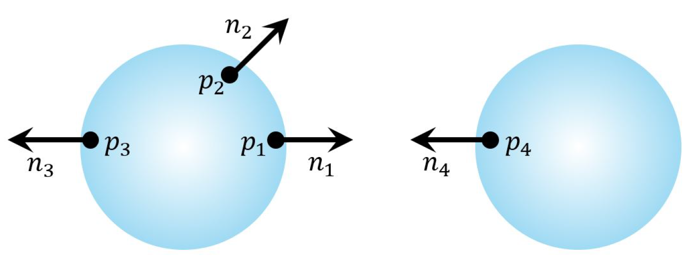
It can be seen that the particles in the adjacent region of the convex-shaped separated droplets have normal vectors in the opposite direction. However, particles inside a droplet can have a small but unpredictable normal vector, and surface particles of the same droplet can have opposite normal directions (see Figure 7). Therefore, we propose a model to distinguish between the particles of the separated droplet by considering two more conditions. To implement this, the function representing the phase of the particle is designed as follows (see Equations (6) and (7)).

$$b_{ij}={\mathbf{n}}_i·{\mathbf{x}}_{ij}{W}_{ij}$$

(6)

$$C_{ij}^n=\left\{\begin{array}{cc}0\hfill & ,\mathrm{if}{b}_{ij}+b_{ji}<\eta \hfill \\ 1\hfill & ,\mathrm{else}\hfill \end{array}\right.$$

(7)

where $\eta$ is a threshold with a negative value to distinguish conditions: If the sum of the state values (b) of the two particles is less than $\eta$, they are considered to belong to different droplets. If the threshold is too small, particles inside the same droplet can be recognized as belonging to different droplets, and if the threshold is too large, particles belonging to different droplets cannot be distinguished.

If the two particles belong to the same droplet, they should affect each other, and if they are considered different phases by belonging to separate droplets, they should not affect each other. To have these constraints, we calculate the force according to the particle area as follows (see Equation (8)).

$$\Delta {\mathbf{p}}_{ij}=C_{ij}^n\left(\Delta {\mathbf{p}}_{ij}^p+\Delta {\mathbf{p}}_{ij}^s\right) + \Delta {\mathbf{p}}_{ij}^{ap}$$

(8)

As the simulation progresses, the particle position is changed and the regions of each other can overlap, so the inclusion relationship was not considered for the artificial pressure to maintain a constant distance according to the repulsive force of each other.

When two particles with different phases approach closer than the radius of the smoothed kernel, the normal vector is smoothed by the adjacent particles and their direction becomes indistinct. Therefore, since it is difficult to express perfect separation of the normal vector with the conventional method, we calculate the normal vector as follows, using the particle inclusion condition at the previous step (see Equation (9)).

$${\mathbf{n}}_i^n=\sum _j{C}_{ij}^{n-1}\frac{m_j}{{\rho }_j^n}\nabla W\left(\left|{\mathbf{x}}_{ij}^n\right|\right)$$

(9)

The calculated normal vector ensures that the particles in the area separated at the previous time-step are not affected at the next time-step. This prevents the normal vector from being smoothed, allowing the droplet to maintain a separate shape in the adjacent region.

We modify C as follows to compute a normal vector that allows the separated droplets to slowly merge over time (see Equation (10)).

$$C_{ij}^n=\left\{\begin{array}{cc}\frac{1}{1+\zeta \left(\eta -b_{ij}-b_{ji}\right)}\hfill & ,\mathrm{if}{b}_{ij}+b_{ji}<\eta \hfill \\ 1\hfill & ,\mathrm{else}\hfill \end{array}\right.$$

(10)

where $\zeta$ is the merging control constant. If $b_{ij}$ and $b_{ji}$ increase, the value of $C_{ij}^n$ converges to 0 and the mutual influence decreases. This modified $C_{ij}^n$ is progressively smoothed into different phases of adjacent regions over time. This induces different phases to change to the same phase, therefore controlling the liquid to naturally merge.

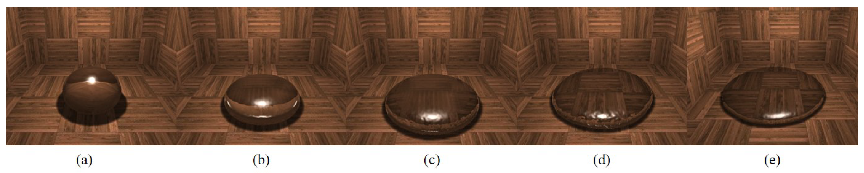
Figure 8 shows the result of controlling the surface tension using our method. In the previous method, droplets are simply merged as they become closer (see Figure 8a), but our method can effectively express non-merging effects without multi-phase simulation (see Figure 8b). In addition, it is possible to express the progressive mixing of droplets with each other through merging control (see Figure 8c). These results can be easily controlled by changing the value of $\zeta$ described before.

3.4. Controlling the String-Shaped Artifact

The pressure force of the SPH keeps the density of the particles constant by regularly disposing the water particles to satisfy the incompressibility of the fluid. However, in the vicinity of the free surfaces, the density is lowered because the number of particles is relatively small, and this low density causes a strong attraction force between the particles to generate clustering artifacts. To reduce these artifacts, the distance between the particles is kept constant by artificially applying a repulsive force between the particles. However, when the artificial pressure is strong, string-shaped artifacts occur because the split fluid tries to forcefully maintain the distance from the adjacent particles (see Figure 3a). Artificial pressure continuously tries to repel adjacent particles, and pressure forces apply an attraction force to the particles as they move away to prevent the density from dropping. The two forces applied in opposite directions create string-shaped artifacts. These artifacts not only make the fluid look very viscous, but when it is accompanied by strong surface tension, the water droplets are expressed in a very unrealistic appearance.

To reduce these string-shaped artifacts, we investigate the particle distribution and reduce the magnitude of the pressure force on the particles in the area where the string shape will occur. Anisotropic kernel approach was used to calculate the distribution of particles adjacent to each particle [56], and the covariance matrix is calculated as follows (see Equation (11)).

$$Co{v}_i=\frac{{\sum }_j\left({\mathbf{x}}_j-{\breve{\mathbf{x}}}_i\right){\left({\mathbf{x}}_j-{\breve{\mathbf{x}}}_i\right)}^T{w}_{ij}}{{\sum }_j{w}_{ij}}$$

(11)

where ${\breve{\mathbf{x}}}_i$ is the weighted mean of the particles: ${\breve{\mathbf{x}}}_i=\frac{{\sum }_j{\mathbf{x}}_j{w}_{ij}}{{\sum }_j{w}_{ij}}$. However, in order to reduce the number of iterations of the neighbor search operation, we approximated it with ${\breve{\mathbf{x}}}_i\cong {\mathbf{x}}_i$. And the isotropic weighting function was used for $w_{ij}$. For each particle, by calculating the SVD (singular value decomposition) for $Co{v}_i$, the direction in which the particles are distributed can be obtained. Since we only need the magnitude of the directionality, we use only the eigenvalue and use the ratio to calculate $d_i$, the weight value of the string shape (see Equation (12)).

$$d_i=\frac{{\sigma }_{i,1}}{{\sigma }_{i,2}}$$

(12)

where ${\sigma }_i$ is the eigenvalue of $Co{v}_i$ and satisfies the condition of ${\sigma }_{i,1}\ge {\sigma }_{i,2}\ge {\sigma }_{i,3}$. Therefore, the above equation indicates the distribution ratio for the 1st and 2nd major axes of adjacent particles with a range of $d_i\ge 1$. This value becomes close to 1 when the particles are evenly distributed in two main axes, and increases as the particles are distributed in only one direction and is closer to a one-dimensional string shape (see Figure 9).

Figure 10 shows the change of $d_i$ according to the shape formed by the movement of the particles. After placing the particles in the 1.5h region, the change in $d_i$ was observed while moving them so that a string shape appeared. As the particles move closer to the string shape, the $d_i$ increases. The red particles in the middle of Figure 10d are the string-shaped areas found by calculating $d_i$, and the $d_i$ of this area is as follows: $d_i\ge$ 1.5. To verify the string shape detection, the particles were arranged in a normal distribution, and the y value converges to 0 as the x value approaches 0 (see Equation (13)). No mutual forces or external forces between particles was applied, and the particles were updated according to the x values of the particles as follows.

$$(x,y)\leftarrow (x,\exp (-\delta -\left|x\right|\left)y\right)$$

(13)

where $\delta$ was used as 5.0.

We use the string shape weight $d_i$ calculated from the covariance matrix to determine the weight of the particles for the pressure force. To allow the force between adjacent particles to be applied symmetrically, the related pressure weight $e_{ij}$ is calculated as follows (see Equations (14) and (15)).

$$\Delta {\mathbf{p}}_{ij}^p\leftarrow e_{ij}\Delta {\mathbf{p}}_{ij}^p$$

(14)

$$e_{ij}=\min \left(\frac{1}{s\left(d_i-1\right)\left(d_j-1\right)},1\right)$$

(15)

where $e_{ij}$ is a value in the range $\left[0,1\right]$ and is determined by the string shape weights $d_i$ and $d_j$ of the two particles. In our method, if it is determined that the region where the two particles are located has a string shape, the value of $e_{ij}$ is reduced to be close to 0, so that string-shaped artifacts are broken in the region. In addition, s is a parameter that controls the attenuation of the force according to the weight of the string shape, and was set to 0.0∼0.5 in all experiments.

4. Implementation Details

The experimental results of this paper were implemented in the following environment: Intel i7-5820k 3.30 GHz CPU, 16 GB RAM and Nvidia GeForce GTX 3060 Ti graphics card. The PBF method [18] was used as a pressure solver for the underlying fluids, and all solutions were implemented based on GPU. For the post rendering scene, 3DMax’s i-ray plugin was used, and for the interactive result, the rendering technique of Wladmir J. et al. [57] was used. Pseudo-code of our foam simulation algorithm is shown in Algorithm 1.

Algorithm 1: Simulation Loop

5. Results

In this paper, we compared the proposed method in 10 different scenarios to analyze it in various ways. First, as a simple test scenario to prove the superiority of the proposed technique, a scene of dropping a spherical liquid on the floor was produced. In this scene, the time-step is set to 0.02, and about 32 k fluid particles are used. We compare the quality of surface tension through PBF [18], Akinci et al.’s technique [34] and the proposed technique.

Figure 11a shows the results of liquid simulation using the technique of Akinci et al. [34]. This approach can stably express the surface tension in a static form, but when a strong external force occurs, the expression of the surface tension becomes unstable due to a rapid change in curvature. According to the results of Akinci et al., in Frame 20, the curvature is minimized according to the surface tension force because it is just before the collision on the ground, but in Frame 46 immediately after the collision, the unstable surface tension is shown by the repulsive force. This problem affects subsequent frames and leads to breakup of the shape maintained by the surface tension (see Frames 74 and 120). On the other hand, our method shows the result of preserving the surface tension shape stably even immediately after collision (see Figure 11b). Figure 11c is the result of assuming high surface tension, and our method stably expresses the multiscale surface tension effects well.

Figure 12 shows the result of high surface tension experiment on concave surfaces. Whereas the previous method produced string-shaped artifacts along the concave surfaces (see Figure 12a), our method stably expressed the high surface tension (see Figure 12b). These results were also shown on convex surfaces (see Figure 13). In addition, our method expressed the high surface tension better than the previous method regardless of the shape of the surface, even though the repulsive force according to the curved shape of the surface was applied immediately after the collision with the surface (see Figure 12 and Figure 13).

To verify whether high surface tension can be stably expressed using this study, a large static water droplet was simulated and the average and maximum values of its curvature were measured while continuously increasing the surface tension constant $\gamma$. The method proposed by Müller et al. [16] was used to measure the curvature: $\left(\nabla ·{\widehat{\mathbf{n}}}_i\right)$.

This is because the average curvature value is lower as the surface tension of the water droplet becomes stronger, and the maximum curvature value increases when the surface of the water droplet vibrates unstable due to excessive force. We calculated the average and maximum values of curvature while constantly increasing the surface tension constant every 100 frames.

We compared how much greater our method can express the surface tension compared to the previous method (see

Table 1. Comparison of changes in curvatures between our method and the previous method (see Figure 14).

	$\mathbf{\Delta }\mathit{t}$: 0.01	$\mathbf{\Delta }\mathit{t}$: 0.03	$\mathbf{\Delta }\mathit{t}$: 0.06	$\mathbf{\Delta }\mathit{t}$: 0.1	$\mathbf{\Delta }\mathit{t}$: 0.15
Minimum avg. curvature ${\kappa }_{ours}$ (our method)	4.52 ($\gamma$: 0.0042)	4.77 ($\gamma$: 0.015)	5.39 ($\gamma$: 0.027)	112.1 ($\gamma$: 0.071)	441.0 ($\gamma$: 0.04)
Minimum avg. curvature ${\kappa }_{N.Akinci}$ [34]	5.47 ($\gamma$: 0.0039)	6.9 ($\gamma$: 0.021)	9.71 ($\gamma$: 0.022)	348.5 ($\gamma$: 0.029)	550.6 ($\gamma$: 0.039)
$\frac{{\kappa }_{N.Akinci}}{{\kappa }_{ours}}$	1.21	1.44	1.8	3.1	1.24

). Comparing the average minimum curvature from small time-step (0.01 s) to large time-step (0.15 s), it was found that our method can stably express a curvature that is 20% smaller than the previous method. In addition, it was confirmed that our method can express the minimum curvature of up to 3.1 times as the time-step increases. However, when the pressure solver itself became unstable due to the time-step being too large (0.15 s), the efficiency decreased, but our method was still able to stably express a larger surface tension than the previous method.

As shown in Figure 15, in the previous method, it can be seen that the surface tension coefficient immediately diverges when it exceeds the limit of minimum curvature. On the other hand, in our method, it can be seen that although there is a slight oscillation near the coefficient that exceeds the minimum curvature, it maintains a stable state after that.

Figure 16 is a sprinkler scene to control string-shaped artifacts in various ways. In the dynamic environment where the water stream spreads, the string shape and droplet generation according to the change of the control coefficient s were examined. As the s controlling the string-shaped artifact increases, the string shape decreases, and it can be seen that more small droplets are generated. However, if s is too large, the particles on surfaces that are repulsed by the ground are torn from the droplets and scattered.

Figure 17 compares the liquid metal expressed using our method and the actual liquid metal. As shown in the figure, the adjacent droplets do not merge with each other and maintain a separate shape.

Figure 18 shows various scenes with multiscale surface tension effects using our method. In the ‘Leaves’ scene, not only a thin stream of water, but also the high surface tension of the tip was well expressed (see Figure 18a). Similarly, in the ‘Water tab droplet’ scene, droplets of various sizes were well expressed (see Figure 18b).

To verify the multi-scale surface tension of our technique, we observed the fluid movement by changing the surface tension constant $\gamma$, string-shaped artifact control constant s, and the boundary shape to open or closed in real time (see Figure 19). It was confirmed that stable results can be obtained even if each parameter is controlled in real time according to the user’s intention regardless of the high or low surface tension.

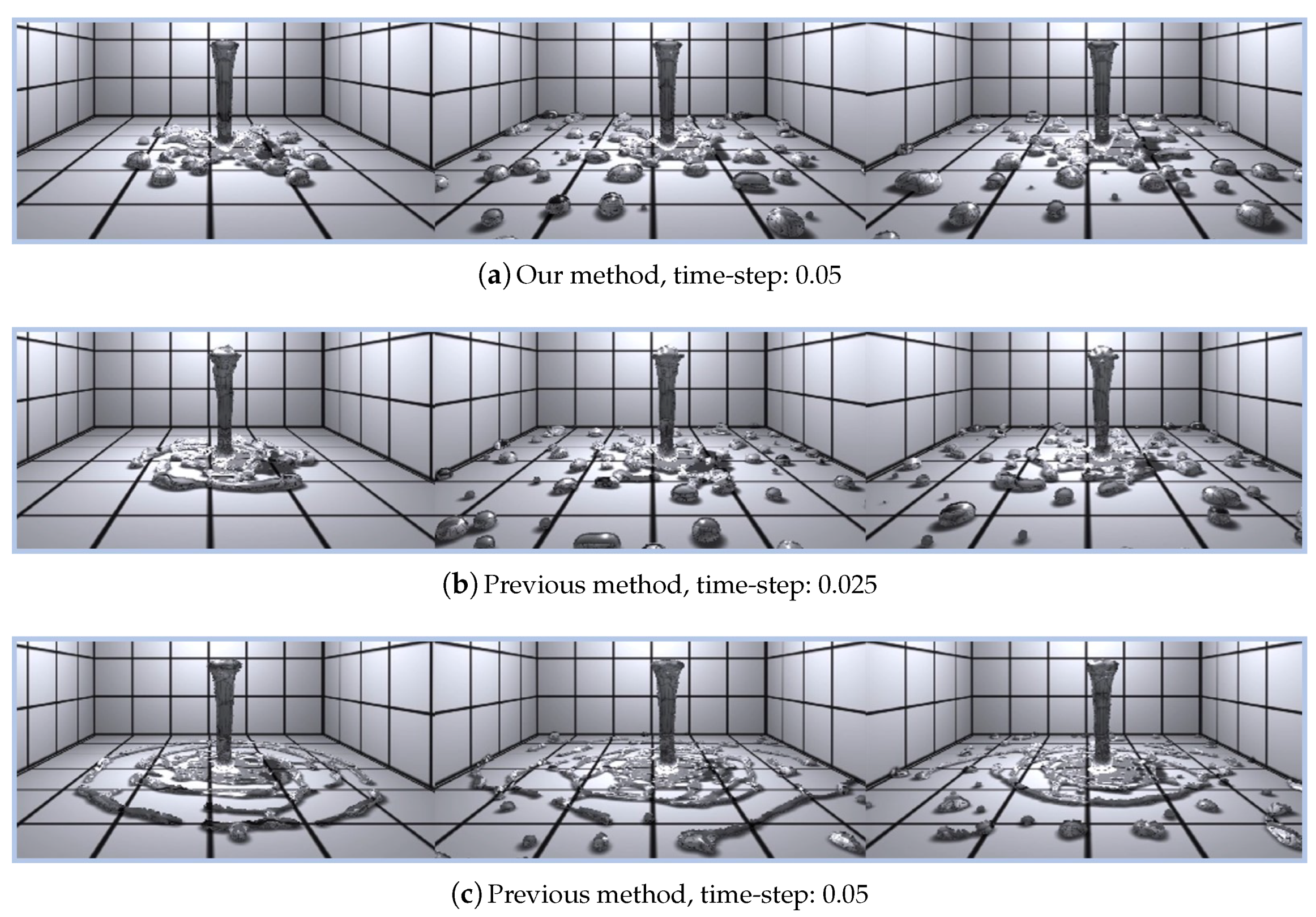
We compared the performance through the same scene with the previous technique (see Figure 20). Our technique used a time-step of 0.05 (see Figure 20a), and the previous technique used a time-step of 0.025 (see Figure 20b). It can be seen that the two results express the similar feeling of surface tension. However, it can be seen from

Table 2. Environment variables for various scenes.

Figure	# of Particles (max)	Time-Step (s)	Steps/Frame (ms)	Time/Step (ms)	Time/Frame (ms)	Iters/Step
Figure 11b,c	32 k	0.02	4	4.5	17.9	4
Figure 12b	150 k	0.03	5	7.2	35.8	4
Figure 13b	140 k	0.03	5	7.0	35.2	4
Figure 14	32 k	0.01∼0.15	5	4.7	23.6	5
Figure 16	180 k	0.03	5	6.3	30.15	3
Figure 17a	230 k	0.01	10	15.8	158.3	5
Figure 18a	310 k	0.01	10	19.6	196.0	5
Figure 18b	130 k	0.02	8	9.0	72.0	5
Figure 19	120 k	0.03	3	10.6	31.9	5
Figure 20a	50 k	0.05	3	7.3	22.0	7
Figure 20b	50 k	0.025	6	5.1	30.8	5
Figure 20c	51 k	0.05	3	7.1	21.4	7

that our method requires about 29% less computational cost than the previous method using a large time-step. In addition, Figure 20c shows the result of applying the same time-step of 0.05 as ours to the previous method. The performance is similar to our technique, but it can be seen that the high surface tension is expressed in an unstable form.

In Table 2, $Time$ is the computational cost of the simulation, i.e., the calculation costs for one time-step and one frame were described. In addition, $Iters/Step$ is the number of iterations of the PBF pressure solver. The simulation computation cost is the computation time excluding the solid-fluid coupling process, and most of the scenes are interactively (less than 66 ms computation time per frame: about 15 fps) executed except for the scenes to which a few postprocesses are applied.

Table 3. Simulation parameters.

Name	Description	Value
$\Delta$t	Time-step	0.01∼0.15
$\gamma$	Surface tension coefficient	0.001∼0.05
$\zeta$	Mering control coefficient	0.0∼5.0
$\eta$	Threshold of phase classification	−2.0∼−1.0
s	String-shaped artifact control coefficient	0.0∼5.0

shows the parameters used to produce the experimental results in this study.

6. Conclusions and Future Work

In this paper, we proposed a framework that can interactively express multiscale surface tension. To improve the instability that occurs when excessive force is applied in the existing technique and to take advantage of the characteristics of the surface tension, the phases were divided. In addition, the droplet shape due to surface tension is realistically expressed by controlling string-shaped artifacts that often occur in PBF. Since our technique was developed based on PBF, its effectiveness when applied to other techniques such as SPH has not been verified. Additionally, since our proposed phase classification method is very sensitive to parameters, it is necessary to experimentally find the optimal parameters for each scene. We treated the different water droplets separately assuming they belong to different phases, and since we did not actually perform multiphase simulation, it is difficult to express water droplets that seem to be torn by air pressure or liquid sheets.

In the future, we will study multiscale surface tension applicable to general iterative pressure solver methods such as PCI SPH, IISPH, and DFSPH. In addition, we plan to expand the study to interactively express fluid properties such as viscosity and vorticity on a multiscale as well as surface tension.