Article

Application of Anti-Diagonal Averaging in Response Reconstruction

Centre for Asset Integrity Management (C-AIM), Department of Mechanical and Aeronautical Engineering, University of Pretoria, Pretoria 0002, South Africa
*
Author to whom correspondence should be addressed.
Symmetry 2021, 13(7), 1165; https://doi.org/10.3390/sym13071165
Submission received: 27 April 2021 / Revised: 17 May 2021 / Accepted: 2 June 2021 / Published: 28 June 2021
(This article belongs to the Special Issue Advanced Mathematical and Simulation Methods for Inverse Problems)

Abstract

:
Response reconstruction is used to obtain accurate replication of vehicle structural responses of field recorded measurements in a laboratory environment, a crucial step in the process of Accelerated Destructive Testing (ADA). Response Reconstruction is cast as an inverse problem whereby an input signal is inferred to generate the desired outputs of a system. By casting the problem as an inverse problem we veer away from the familiarity of symmetry in physical systems since multiple inputs may generate the same output. We differ in our approach from standard force reconstruction problems in that the optimisation goal is the recreated output of the system. This alleviates the need for highly accurate inputs. We focus on offline non-causal linear regression methods to obtain input signals. A new windowing method called AntiDiagonal Averaging (ADA) is proposed to improve the regression techniques’ performance. ADA introduces overlaps within the predicted time signal windows and averages them. The newly proposed method is tested on a numerical quarter car model and shown to accurately reproduce the system’s outputs, which outperform related Finite Impulse Response (FIR) methods. In the nonlinear configuration of the numerical quarter car, ADA achieved a recreated output Mean Fit Function Error (MFFE) score of 0.40 % compared to the next best performing FIR method, which generated a score of 4.89 % . Similar performance was shown for the linear case.

1. Introduction

In the drive for continual improvement in vehicle engineering design, optimised structures and components with lower safety margins and greater reliability are sought [1]. Advances in computational design such as finite element analysis and dynamic modelling combined with fatigue prediction have furthered this goal tremendously during the design phase. Nevertheless, there is still a need to dynamically test physical prototypes or existing designs in a controlled laboratory environment. For the analysis to be worthwhile the excitation of the structure in the laboratory environment must induce responses in the structure as though it were being tested under real-world operating conditions. The end goal is to enable Accelerated Destructive Testing (ADT) of the structure. In ADT, a vehicle’s chassis is mounted with its suspension system on a set of hydraulic actuators. The hydraulic actuators then excite the system vertically. Laterally acting forces are simulated with additional actuators. An example of an ADT set-up is shown in Figure 1.
The structure’s excitation is then carried out for extended periods, allowing for the degradation of the structure to be measured in a controlled environment [1]. The structure is not typically excited until catastrophic failure, but rather until the degradation measured as vibration or noise has met a specified threshold [2]. This indicates possible failure points of the system and a means of predicting the component’s healthy lifespan. Other insights can be gained from dynamic testing, such as a better understanding of the system dynamics, vibration isolation [1] and vibration severities for passenger ride comfort [3].
The biggest hurdle with ADT is that the inputs to the system, such as the displacements or the forces acting on the vehicle’s tyres, are difficult or impossible to measure directly in the field. This means the problem must be cast as an inverse modelling or response reconstruction problem [4]. In inverse problems, the outputs of the system Z are used in conjunction with model parameters β to determine the inputs U, i.e.,
U = f ( Z , β ) .
There are two possible choices for creating a model of the system. A mapping of the system can be constructed so that the system’s inputs are used to predict the outputs of the system. This is referred to as the forward problem. The forward problem is then inverted. If the model used to map the problem is nonlinear, an iterative optimisation scheme is employed to invert the system. However, the optimisation scheme may be prone to local minima. The second approach is to create a direct inverse of the model whereby the system’s outputs are used to predict the inputs of the system. The inverse method has an inherent stability check since the solution will only be obtained if the direct inverse model is stable [1]. However, we quickly find that most inverse problems are ill-posed. For a problem to be well-posed it needs to meet the following criteria: the solution is unique, the global solution exists for all data and the solution to the problem is continuously dependent on the given data [5]. The first criterion is normally the offending culprit since it is easy to construct a forward problem where two different inputs result in the same output. Therefore, the inverse solution is typically not unique. This introduces an asymmetry into the problem whereby the assumption of an one-to-one mapping is broken. If the problem is ill-posed we may use regularisation techniques to cast the problem as a more well-behaved problem. Regularisation techniques include: cross validation, SVD, iterative methods, data filtering and Tikhonov regularisation [4].
Most common reconstruction techniques are implemented in the frequency domain [6], whereby the discrete Fourier response is multiplied by an inverse or pseudoinverse frequency response function [7]. Raath’s Ph.D. thesis [1] highlighted the then known issues of using frequency response techniques in accelerated fatigue testing. It was shown that the frequency response was inaccurate for several reasons, that include:
  • Assuming that the input and output signals are periodic when often they were not. These include sharp impulses from random impacts.
  • Being unable to model nonlinear models since frequency response analyses assume a linear model.
  • Requiring long time signals of the order of hours as opposed to minutes or seconds needed for the time domain. This ties in with the issue that low frequency information is easily lost due to spectral leakage where the energy in the lower frequencies is spread over to higher frequencies.
  • Failing to capture the sequence or causal effects which play an important role in crack propagation.
Various time-domain techniques have been developed to overcome this. However, they have been shown to be slow or inaccurate [8]. The vehicle structures of interest typically contain many nonlinear components such as springs and pneumatic dampers. Typical control systems will overcome this issue by linearising the system around the operation point. It is then assumed that the system will experience small perturbations around this point. However, it is expected that the system will experience impact loadings and large displacements, which will force the system out of its linear region [1]. Another issue associated with response reconstruction is that of model mismatch, whereby the identified system does not truly represent the physical test rig. In response reconstruction the misrepresentation occurs when the physical test rig is taken from the real-world and recreated and simulated in the laboratory environment. Typically the degrees of freedom are not fully represented in the laboratory or the test rig parameters, such as mass, may vary. In this laboratory environment, the process of system identification occurs; therefore, we will have mapped a domain that differs from the real-world domain. When the real-world outputs need to be recreated we may find that the mapped inverse model may be forced to extrapolate into regions in the mapped domain to find a solution. In other words, the inverse model has over-fitted to the laboratory domain and generalises poorly with regard to the real-world domain. Regularisation can be employed to minimise this error [9]. A related field to response reconstruction is force identification whereby the inputs of the system are of interest. However, the inputs of the system for a given output are not unique [10]. Force identification tackles this problem by enforcing some prior knowledge of the system dynamics to constrain the inputs to reasonable solutions. Bayesian methods have become prevalent in force identification literature since they allow the experimenter to systematically incorporate prior knowledge [11]. Another benefit of incorporating Bayesian methods is that it provides for confidence intervals on the input predictions and model parameters [12]. A noticeable distinction in force identification literature is that a known finite element model of the structure is typically assumed, i.e., a known forward model.
The approach taken in this paper of solving the issue of non-uniqueness of the input is mitigated by
  • not focusing on the reconstructed input accuracies.
  • using cross validation of the system’s reconstructed outputs to determine whether a given inverse model of the system is satisfactory i.e., using a forward pass through the physical system in each cross validation step to determine the model accuracy.
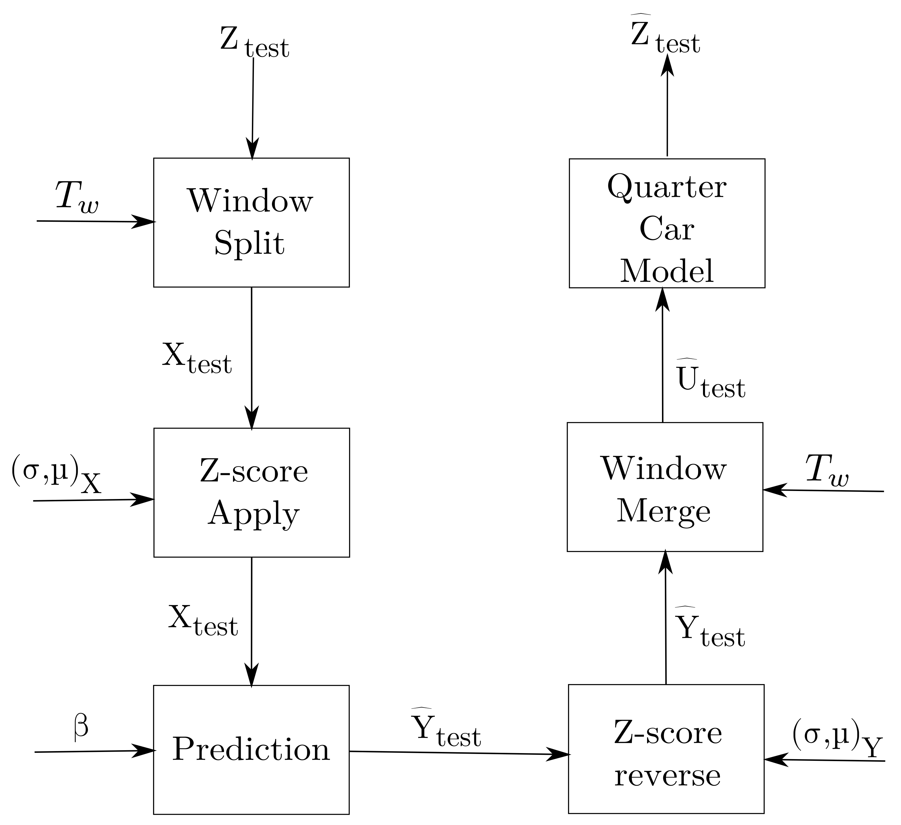
A potential drawback to this approach is that, if implemented naively, the cross validation can induce undue stress on the system before any ADT occurs. An overview of the response reconstruction methodology used in this paper is given in Figure 2.
This paper focuses on linear regression methods for mapping the relationship between the outputs X and inputs Y for response reconstruction, i.e., X β = Y . The core contribution of this paper is the proposed method of extending the capabilities of said linear regression methods by introducing overlaps and merging them using averaging in a process called AntiDiagonal Averaging (ADA), encapsulated in Equation (12). We show that ADA is closely related to FIR methods. We benchmark ADA in terms of its response reconstruction ability as well as its performance against the related FIR methods. We focus on Tikhonov regularisation with cross validation through the use of Ridge Regression (RR) to regularise the inversion of the system. Any suitable linear regression method can be employed with ADA; however, RR is needed for the FIR methods we cover.
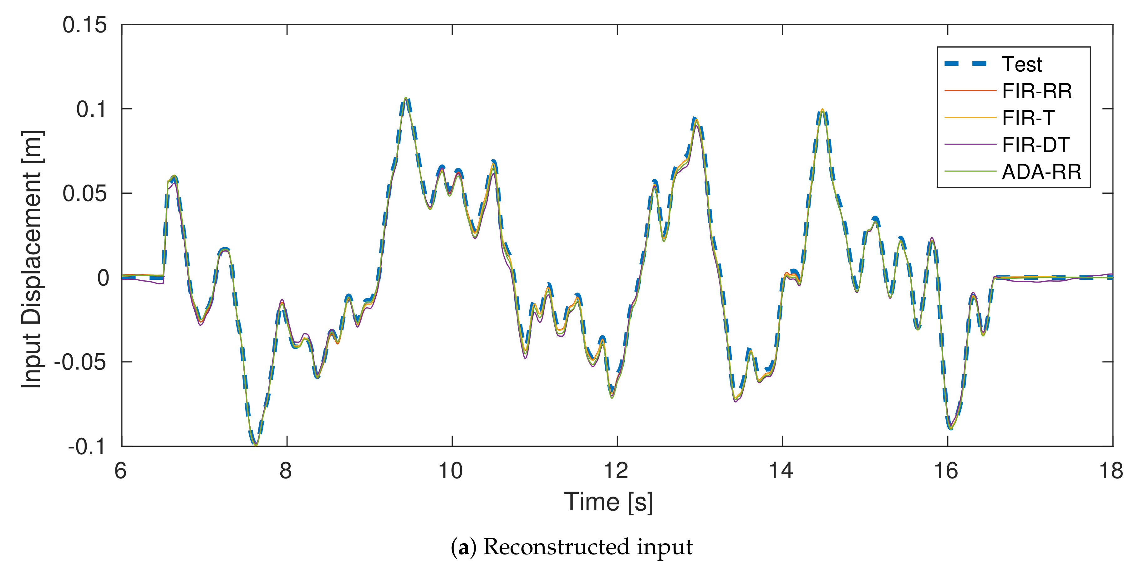
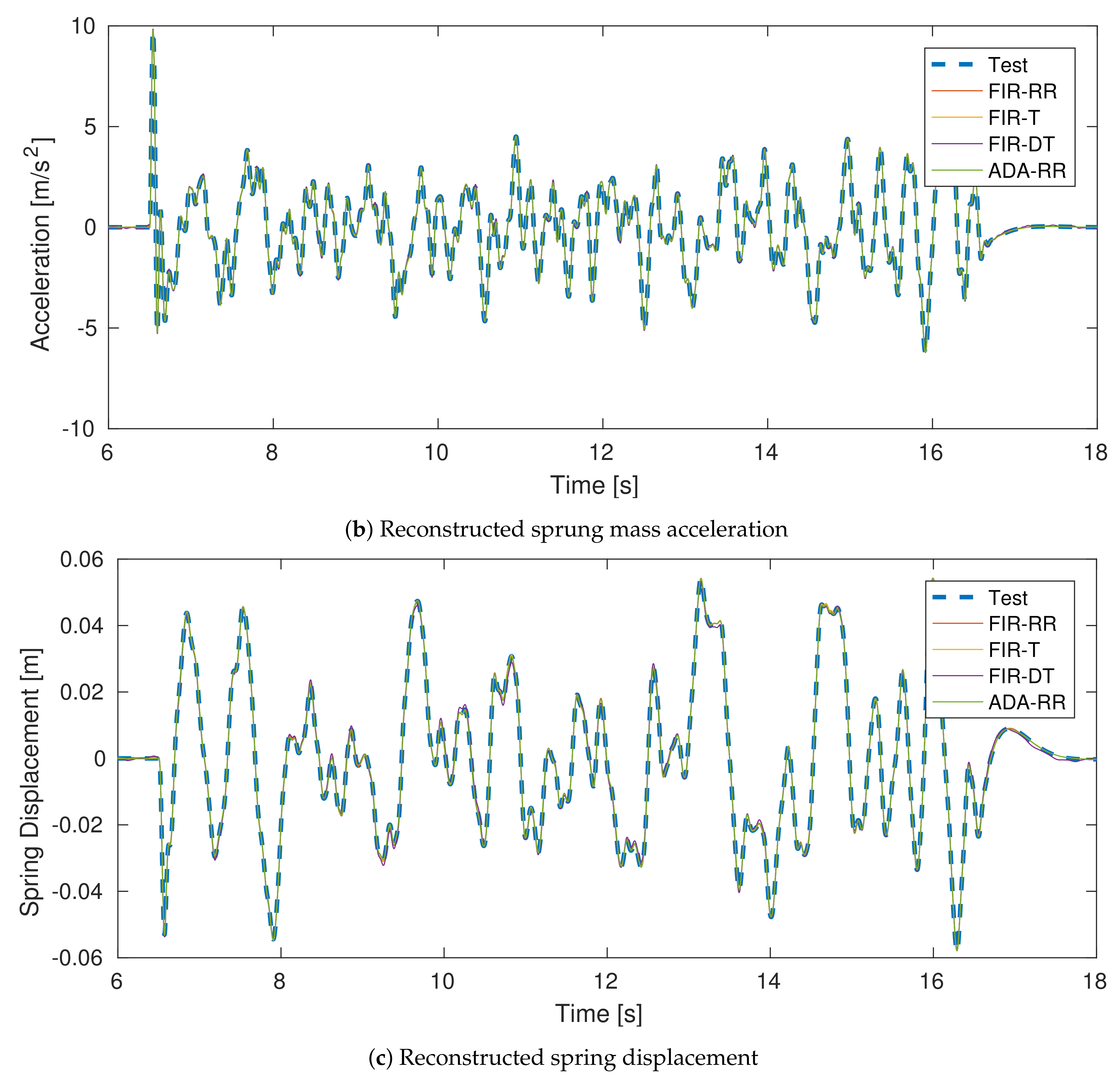
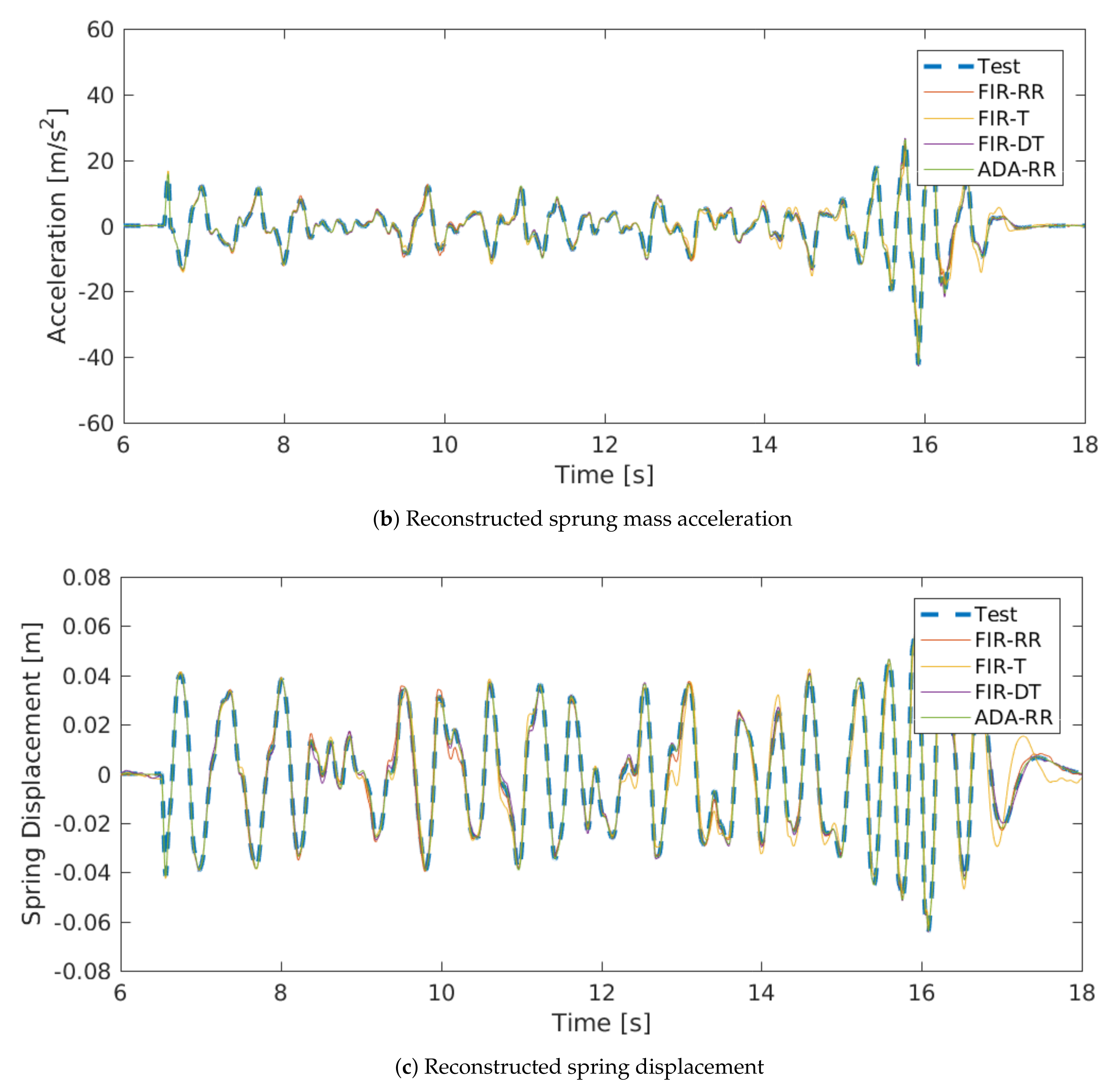
We first give a brief overview of RR and how it enforces regularisation. The theory behind ADA is then introduced and compared against related FIR methods. The design of the investigation is then given with an overview of the numerical quarter car model, with which the reconstruction methods are benchmarked. The results of the benchmarks are then discussed. Finally, an illustrative comparison of the different regression methods is conducted showing the performance of the regression method on a challenging response reconstruction problem.

1.1. Ridge Regression

As opposed to discretely truncating the singular values, RR instead smoothly decays the singular values through the use of a regularisation matrix Γ which results in the solution
β = ( X X + Γ Γ ) 1 X Y ,
where Γ is typically chosen as a scaling of the identity matrix though the use of the regularisation constant α , i.e., Γ = α I . RR has the solution in terms of the SVD of X [13]
Y ^ = X ( V x D U x ) Y ,
where the entries of the diagonal matrix D are given by
D i i = s i s i 2 + α 2 .
U x and V x are the left and right singular vectors of X, respectively, with the corresponding singular values s i .

1.2. ADA

Windowing methods are needed to represent the responses Z as the predictor matrix X R n × p and the inputs U as the target matrix Y R n × r in any suitable linear regression method. This is achieved by windowing said signals and treating each window as an observation. The original input and response measurements are given by U R m × q and Z R m × o where m is the original sequence length in samples and q and o are the number of actuator and sensor channels, respectively.
In ADA we introduce overlap between these observations. The overlap sample length s γ is defined by a proportion γ of the proposed window sample length s w , i.e.,
s γ = γ s w .
where s w is the window sample length given by the desired window length in seconds T w multiplied by the sampling frequency f s
s w = f s T w .
The stride of the window, s τ , is then given by
s τ = s w s γ .
This occurs for each time sequence for either an actuator or sensor signal, being appended column-wise, resulting in
p = s w × o ,
r = s w × q
and the number of rows or observations, n, equal to
n = m s γ s τ .
We set the amount of overlap to the extreme such that the stride is one sample, i.e., s τ = 1 . This results in the following windowed target matrix Y
Symmetry 13 01165 i001
The windowed predictor matrix X takes on a similar form (not shown). We can simply average over the anti-diagonals of the windowed data matrix Y ^ to reconstruct the approximated input U ^ . To compute the average response u ^ ( k ) we average all the anti-diagonal terms of Y ^ i , j , such that
u ^ ( k ) = 1 n diag Y ^ i , j ,
for which i + j = k + 1 and n diag is the number of elements in the anti-diagonal. This process is known as Hankelization which is the same process followed in Singular Spectral Analysis (SSA) [14]. The corresponding windowed matrix is referred to as the trajectory matrix. This is known as the embedding step in SSA. The windowed matrix is then decomposed using SVD. In this case, we are merely borrowing the ADA concept from SSA for the regression problem, whereas SSA typically uses this process for autoregressive models.
An example signal with m = 7 samples and window length s w = 3 and windowed with ADA results in the following equation
u ^ ( 1 ) u ^ ( 2 ) u ^ ( 3 ) u ^ ( 2 ) u ^ ( 3 ) u ^ ( 4 ) u ^ ( 3 ) u ^ ( 4 ) u ^ ( 5 ) u ^ ( 4 ) u ^ ( 5 ) u ^ ( 6 ) u ^ ( 5 ) u ^ ( 6 ) u ^ ( 7 ) = z ( 1 ) z ( 2 ) z ( 3 ) z ( 2 ) z ( 3 ) z ( 4 ) z ( 3 ) z ( 4 ) z ( 5 ) z ( 4 ) z ( 5 ) z ( 6 ) z ( 5 ) z ( 6 ) z ( 7 ) β 1 , 1 β 1 , 2 β 1 , 3 β 2 , 1 β 2 , 2 β 2 , 3 β 3 , 1 β 3 , 2 β 3 , 3 .
Here z is the response signal used to predict the inputs u. The linear coefficients β are computed using any suitable linear regression method. To gain insight into the workings of ADA we can write out the set of equations that infer u ^ ( 3 ) , i.e.,
u ^ ( 3 ) 1 = β 1 , 3 z ( 1 ) + β 2 , 3 z ( 2 ) + β 3 , 3 z ( 3 ) ,
u ^ ( 3 ) 2 = β 1 , 2 z ( 2 ) + β 2 , 2 z ( 3 ) + β 3 , 2 z ( 4 ) ,
u ^ ( 3 ) 3 = β 1 , 1 z ( 3 ) + β 2 , 1 z ( 4 ) + β 3 , 1 z ( 5 ) .
We can then average over all the u ^ ( 3 ) predictions to obtain the final prediction of u ^ ( 3 )
u ^ ( 3 ) = 1 3 u ^ ( 3 ) 1 + u ^ ( 3 ) 2 + u ^ ( 3 ) 3 = z ( 1 ) β 1 , 3 3 + z ( 2 ) β 2 , 3 + β 1 , 2 3 + z ( 3 ) β 3 , 3 + β 2 , 2 + β 1 , 1 3
+ z ( 4 ) β 3 , 2 + β 2 , 1 3 + z ( 5 ) β 3 , 1 3 .
If we rewrite the average of the β multiplying with a particular z term as a new constant, e.g., β 2 = β 2 , 3 + β 1 , 2 2 , we obtain
u ^ ( 3 ) = β 1 1 3 z ( 1 ) + β 2 2 3 z ( 2 ) + β 3 1 z ( 3 ) + β 4 2 3 z ( 4 ) + β 5 1 3 z ( 5 ) .
Here we note that the ADA emphasises the middle term with decreasing emphasis placed on proceeding and preceding terms. It in effect creates a triangular windowing function. If we add a corresponding weight term w, e.g., w 2 = 2 3 we can rewrite the equation generally as
u ^ ( k ) = β 1 w 1 z ( k s w ) + + β s w w s w z ( k ) + + β k + s w w k + s w z ( k + s w ) .
This result demonstrates that ADA is an indirect method of creating a weighted moving average filter. In system identification this is known as a Finite Impulse Response (FIR) model. More specifically this an example of a non-causal weighted FIR model. The weights can be arbitrary and are a prior design choice. If we forgo the ADA method and use the weighted FIR model, we can be more creative with the weighting.

1.3. FIR Models

In FIR models the current output of the system is a function of past inputs such that
z ( k ) = f ( u ( k 1 ) , , u ( k s w ) ) .
This is in contrast to other models such as Autoregressive eXogenous (ARX) which includes output feedback as well, i.e.,
z ( k ) = f ( u ( k 1 ) , , u ( k s w ) , z ( k 1 ) , , z ( k s w ) ) .
This paper focuses on non-causal inverse implementations of FIR models, where the current input is a function of both past and future outputs, written as
u ( k ) = f ( z ( k s w / 2 ) , , z ( k + s w / 2 ) ) .
By using the FIR model, the predictor matrix X takes on the form
Symmetry 13 01165 i002
with the corresponding target matrix Y written as
Y = u 1 ( s w / 2 ) u q 1 ( s w / 2 ) u q ( s w / 2 ) u 1 ( s w / 2 + 1 ) u q 1 ( s w / 2 + 1 ) u q ( s w / 2 + 1 ) u 1 ( m s w / 2 1 ) u q 1 ( m s w / 2 1 ) u q ( m s w / 2 1 ) u 1 ( m s w / 2 ) u q 1 ( m s w / 2 ) u q ( m s w / 2 ) .
It is worth noting that we lose the first and last s w / 2 samples of the target matrix Y since we shifted the inputs to make the system non-causal.
The lack of feedback means that FIR methods are inherently stable. This is suitable and sometimes sought after if the system under consideration is stable. However, if the system is unstable, it will only approximate the instability for a short period before diverging [15]. FIR models come with the cost of needing significantly more terms than what output feedback models need to map the same system [15]. A similar approach to ADA can be achieved through the use of FIR models combined with Tikhonov regularisation. Using Tikhonov regularisation, the β coefficients can be penalised and thus shaped by choice of the Γ matrix in Equation (2). To this end three options for the Γ matrix are implemented in this paper, namely: Finite Impulse Response with TriangularWeighting (FIR-T), Finite Impulse Response with Difference Smoothing and Triangular Weighting (FIR-DT) and Finite Impulse Response with Ridge Regression (FIR-RR).
In FIR-T, the coefficients relating to the outputs further away from the required input (both forwards and backwards in time) are penalised. This is achieved by setting
Γ Γ = α W
where W is an inverted triangular set of penalty weights, given as
W = d i a g s w / 2 s w / 2 1 2 1 2 s w / 2 1 s w / 2 ,
and α scales the amount of regularisation we wish to impose. This should ideally mimic the weighting function achieved by ADA in Equation (20). FIR-DT further modifies the triangular weighting matrix through the use of a first difference matrix A, given as
A = 1 0 0 0 1 1 0 0 0 1 0 0 0 0 1 1 .
The first difference matrix ensures that the difference between each successive β coefficient is small [16]. The difference matrix is then combined with the weighting matrix W to obtain the final form of the regularisation matrix such that
Γ Γ = α A W A .
This weighting scheme was initially implemented and developed for a causal FIR system where the penalty weights increased linearly further back in time [16]. Finally, the last choice of penalty matrix Γ is that of FIR-RR, i.e.,
Γ = α I
where we only limit the magnitude of the weights to act as a reference. This enables us to determine whether the regularisation of β contributes to the accuracy of the response reconstruction.

2. Method

This section describes the general experimental design procedure for the numerical investigations.

2.1. Numerical Quarter Car Model

A simple two-degree-of-freedom nonlinear mass–spring–damper system, representing a quarter car model is used to investigate the methods explored in this paper. The numerical model employed is shown schematically in Figure 3. The sprung mass M A and unsprung mass M R represent the mass of the vehicle’s body and the suspension–tyre system, respectively. These bodies are connected by springs and dampers, which represent the dynamics of the suspension system. The unsprung mass is then connected to the road via a spring characterising the tyre stiffness. The system is excited by a road profile u road .
The system behaves according to the following equations of motion:
z ¨ A = b A M A ( z ˙ A z ˙ R ) k N L M A ( z A z R ) 3 k A M A ( z A z R ) ,
z ¨ R = + b A M R ( z ˙ A z ˙ R ) + k N L M R ( z A z R ) 3 + k A M R ( z A z R ) k R M R ( z R u r o a d ) ,
where the k and b terms are the stiffness and damping coefficients, respectively. The nonlinearity is introduced by having cubic stiffening of the sprung mass spring controlled by the k N L term. The sprung mass spring force, f A , is given by
f A ( Δ z ) = k A Δ z k N L Δ z 3 ,
where we define a new state of the system representing the deflection of the spring, Δ z , such that
Δ z z A z R .
The k N L term can be varied to change the severity of the system’s nonlinearity or switch it completely off for linear behaviour. A hardening spring is modelled by choosing k N L > 0 . This results in a spring that becomes stiffer as it undergoes compression or tension. Likewise, a softening spring can be implemented by choosing k N L < 0 . In this study the linear component will always be restorative such that k A > 0 . The default parameters chosen for the numerical quarter car are given in Table 1.

2.2. Choice of Excitation Signals

Before we can begin building a direct inverse model of our plant we need informative data since the excitation signal’s quality places an upper bound on the accuracy of any subsequent model that we wish to build [15]. For response reconstruction, we can design the signals on which we want to train. There are two possible methods of designing excitation signals: model-free and model-based methods. In model-based methods subsequent excitation signals are chosen to improve the accuracy of the model [17]. In model-free methods we design an excitation signal that offers the best distributed coverage of the operating condition. Initially we have little prior knowledge of the system and of the real world input signals; therefore, we need to employ model-free methods. We assume we have some prior knowledge of the range of the operating condition. A suitable choice is the Amplitude Modulated Pseudo Random Binary Signal (APRBS).

2.2.1. Amplitude Modulated Pseudo Random Binary Signal

Since we are working with nonlinear structural systems, we know that the system responses are functions of input frequencies and the amplitude at which we excite the system. Therefore a signal that covers the necessary frequencies and the expected amplitude range of operations is required. The APRBS attempts to cover the amplitude operating conditions with a series of step responses that are fairly well distributed over the input range. An example of an APRBS is shown in Figure 4.
To specify the profile, a set of N design points d n are chosen to define the step’s amplitude. The design points are sampled from the desired range [ u min , u max ] using Latin Hypercube Sampling (LHS). LHS splits the design space into N intervals with one design point placed randomly in each interval. LHS then iteratively optimises the design points such that each design point is the maximum distance away from its neighbours. This provides a random but equally spread set of design points. Since no physical system can achieve an instantaneous change in displacements required for a true step input, the step is instead approximated by a ramp function. The slope of the ramp is determined by the maximum allowed velocity v max that can safely or accurately be performed by the actuator. The ramp’s slope affects the frequency content of the signals with higher velocities resulting in higher frequencies being excited [18]. The length of the step is then specified by the hold time T h . Since the testing time is limited, the maximum number of steps that best cover the input space in the shortest time is sought. The hold time T h must be small enough to fit as many steps in but must be long enough that the steps actively excite the system at that point. The hold time T h is typically set to be at least the length of the largest time constant T c , max of the system [15]. This can be determined with a simple step test of the system if no prior knowledge is known. The parameters used for the investigations are given in Table 2.

2.2.2. Road Profile

The ISO 8608 standard [19] for specifying road profiles is used to generate a separate test set to determine how well the direct inverse model performs on unseen data. The ISO 8608 standard defines inputs that are distinct from APRBS while still being representative of real-world operating conditions. The profiles are characterised by the standard in the frequency domain where the spectral density S z is given by
S z ( ϕ ) = A ( ϕ ) n ,
for the given spatial frequency ϕ with units m 1 . The A term represents the road’s roughness coefficient, whereas n represents the road index of the profile. The A coefficient controls how large the amplitudes are at each frequency whereas n controls how quickly the amplitudes decay as frequency functions. Varying types of profiles such as ploughed agricultural land to smooth gravel highways can be produced by altering these two coefficients. The spatial frequencies ϕ are limited between 0.5 and 10 m 1 . The former represents the broad changes in the landscape which have negligible effects on vehicle dynamics. In contrast, the upper limit on the frequency represents small variations which are filtered out by the tyre [20]. When generating the profiles only the amplitude information is given by the ISO 8608 standard; therefore, in order to generate time signals, a uniformly random signal is generated for the phase signal with spatial frequencies sampled at discrete intervals. This generates a displacement signal as a function of distance. The vehicle’s velocity must be chosen to generate a displacement signal as a function of time. The parameters of the road profile used are given in Table 3.

2.2.3. Preprocessing

The windowing techniques covered in this paper will truncate some of the testing and training set samples. To ensure a fair comparison between the different data sets, a dead time is appended and prepended. The dead times will be excluded when calculating the cost function during cross validation and reporting the final accuracy of the predictions. The constant initial and final conditions also allow for different signals to be concatenated without introducing unwanted jumps.

3. Scaling

The windowed inputs Y and windowed outputs X of the system record different types of signals which will have different variances across them. We may also find that constant biases need to be accounted for from the sensors. Therefore, the inputs and outputs are z-scored normalised to scale the rows to have a mean of zero and a variance of one [13].

4. Cross Validation

To determine the optimal regularisation constant α for RR, cross validation is used. However, cross validation can be misleading if it is implemented without considering the correlation between observations. Suppose the validation set is removed once the data have already been windowed with overlaps. In that case, the validated set will be correlated to the training set due to the overlaps introduced. If the validation set is first removed from the middle portion of the dataset and then windowed, then care must be taken when splitting and merging the training set to ensure that no unintended overlap is introduced between the separated training segments. A simpler solution to this problem is implemented by removing a single validation set from either the beginning or end of the dataset before windowing. In this work, a validation set was created independently of the training set.

4.1. Choice of Cost Function

We have the choice of either using the errors of the approximated inputs or the approximated outputs as the cost function of the optimisation scheme. In response reconstruction, we are interested in producing an accurate output response since a unique input may not exist. The downside of this is that, to obtain the output error, the approximated input needs to be passed through the test rig. This needs to occur for every loop in the cross validation step. The numerical model is computationally efficient to compute. However, this would result in significant fatigue of the experimental rig in the real world and would take considerable time to run. Therefore, it is necessary to limit the number of forward evaluations in the cross validation step. In evaluating these methods for response reconstruction, the output error is used during cross validation. Since we need to measure and compare response and input reconstruction accuracies across different types of signals, we need a normalised measure of error. The Mean Fit Function Error (MFFE) [21] is used to report the final test accuracies of the reconstructed input and output signals. MFFE is defined as
MFFE = 100 × m = 1 M | e 0 | m = 1 M | z 0 | [ % ] ,
where e 0 is the error between the true output z 0 and the approximate output z ^ 0 , i.e.,
e 0 = z 0 z ^ 0 .
The signals under consideration have been mean centred such that
z 0 = z μ z ,
z ^ 0 = z ^ μ z ^ .

4.2. Training Procedure

The cross validation algorithm consists of two sub-routines: an outer routine that incorporates the windowing parameter grid search for the optimal window length T w and an inner subroutine which optimises the regularisation constant α .

4.2.1. Window Loop

A graphical overview of the training process is shown in Figure 5 with focus on the window parameter search. The window optimisation loops over the window length, T w , i , where i represents the ith iteration of the loop. The training set U train and Z train as well as validation output Z val are then windowed accordingly. The z-score parameters, σ i and μ i , are then calculated using only the training dataset and applied to both the training and validation set. The training set is then decomposed using SVD according to the regression method specified, in this case RR. The decomposed SVD is then passed to the regularisation optimisation loop.

4.2.2. Latent Variable Loop

Figure 6 depicts a graphical overview of the regularisation constant optimisation. The regression coefficients β k are then calculated and weighted with α k , where k is the k t h iteration of the loop. The approximated windowed validation inputs Y ^ val are then predicted using the windowed validation outputs X ^ val . The approximated windowed validation inputs are rescaled and then merged using the specified windowing methods to obtain the approximated input U ^ val . The merged inputs are then passed through the test rig to obtain the approximated output Z ^ val . The MFFE is then calculated between the true output Z val and the approximated output Z ^ val . The optimised regularisation constant α k and the corresponding minimum MFFE are then returned from this loop to the windowing loop as seen in Figure 5. This minimum MFFE result is then used in the window loop to find the corresponding optimal window length T w , min .

4.2.3. Final Training Step

In the final training step, the training set is concatenated with the validation set. This newly combined set is then windowed with the optimised window parameters T w , min . The new z-score parameters [ σ , μ ] are then calculated. The combined set is decomposed and used in the regression step with the optimised regularisation constant α min to determine the final regression coefficients β final .

4.3. Prediction

A graphical overview of the prediction step and the approximation of the output is shown in Figure 7. Once the training step is complete, it is relatively straightforward to use the optimised parameters to make further predictions. The test output signal Z test needs to be preprocessed first before predictions can be made. To obtain the predictor matrix, X test , the test signal is windowed and z-scored normalised using the parameters determined during the training phase. The prediction step then occurs using the regression coefficients β final obtained during training to obtain the approximate target matrix, Y ^ test . The windowing and z-score normalisation are then reversed before passing the approximated input U ^ test into the test rig to obtain the approximated output, Z ^ test .

5. Comparison against Finite Impulse Response (FIR) Models

This section aims to benchmark ADA against FIR in terms of response reconstruction since ADA can be seen as a subset of FIR. The idea behind this benchmark is to ensure that ADA is not an indirect method of achieving an FIR implementation. If so, it needs to be determined whether ADA offers any substantial benefits over using FIR.

5.1. Finite Impulse Response (FIR) Comparison Procedure

The three different regularised FIR implementations will be compared against ADA combined with RR for two different test cases, linear and nonlinear. The experiment will be performed with a system configuration more representative of a typical test rig. In this case the sprung mass acceleration and spring displacement (i.e., the delta between the sprung and unsprung mass) of the quarter car will be used. The first being the linear system and the second being the default nonlinear system. The inputs and responses will be sampled at 250 Hz and 350 Hz for the linear and nonlinear systems, respectively. The window lengths will be determined via grid search cross validation with the window lengths being sampled from T w [ 0.1 , 12 ]   s with a grid of 50 equally spaced intervals. The potential α values used to regularise RR will be spaced equally on a log scale within the range α [ s min × 10 5 , s max ] , where s are the singular values. Thirty equally spaced divisions will be used. An overview of the numerical experiment parameters is given in Table 4.

5.2. FIR Comparison Numerical Results

The reconstructed inputs and outputs for the linear and nonlinear systems are shown in Figure 8 and, Figure 9 respectively. The response reconstruction results for the linear and nonlinear systems are shown in Table 5. We treat FIR-RR as the bare minimum regression method since it does not impose a prior choice on the shape or smoothness of the β parameters.
For the linear case it appears that the imposed smoothness offered by FIR-DT does not contribute any significant improvement and actually hinders the reconstruction performance. If we refer to the optimised hyper-parameters for the numerical experiment in Table 6, we see that FIR-DT used a small amount of regularisation which further indicates the poor suitability of the methodology to the problem. We note that the triangular weighting offered by FIR-T performs similarly to FIR-RR, which suggests that the shape of the β parameters, is not as important for the linear case. However, ADA still performs an order of magnitude better in terms of the recreated output MFFE scores. This suggests, at least for the linear case, that the ADA performance is not necessarily due to the shape factor or due to imposed smoothing of each successive β parameter.
For the nonlinear case, we note that FIR-T, obtains the worst recreated output score with the default regression method, FIR-RR, performing significantly better. This suggests that the introduction of the triangular weighting is ill-suited for the nonlinear case. The introduction of the difference smoothing in the form of FIR-DT is an improvement over FIR-RR, which suggests that the smoothing of the β parameters is an improvement in the FIR regression methods’ performance. If we refer to the optimised hyper-parameters in Table 7, we note that ADA implemented a low amount of regularisation for the nonlinear case. This indicates that averaging used in ADA adds an extra form of regularisation since it performs an order of magnitude better than the other regression methods for the nonlinear case, without relying on a large regularisation constant. This is corroborated by the fact that ADA outperforms the other regression methods when either smoothing is better suited (nonlinear case) or imposing a shape is better suited (linear case), which suggests that the averaging inherent to ADA is the key factor for its performance regarding the problem at hand.
In general, we note that the MFFE results for the recreated outputs of the system (for both the linear and nonlinear case) are lower than their associated input MFFE results. This indicates the non-uniqueness of the inputs for the given response since a seemingly poor input can result in an accurate output. This justifies the need to incorporate the forward pass through the system to determine the suitability of the input by judging it by its associated recreated output.

6. Illustrative Use Case

In this section, we create a scenario whereby all the challenges to response reconstruction are introduced. These are noise, model mismatch and nonlinearity. In this experiment we focus on a narrower scope of model mismatch whereby the model parameters of the system are simply scaled from the real-world environment to that of the laboratory environment. A broader scope of model mismatch would be to add new dynamics going from one environment to the other. One such example would be to add or remove a discontinuity, i.e., a tyre separating from the road surface. This paper focuses on this narrower view of model mismatch. The default parameters given in Table 1 are modified such that
M A , mis = M A 1 m % 100
M R , mis = M R 1 + m % 100
b A , mis = b A 1 m % 100
k A , mis = k A 1 + m % 100
k R , mis = k R 1 m % 100 .
The investigation is not exhaustive but rather proposed to give an illustrative sense of the regression methods’ performance on a challenging response reconstruction problem. To this end, the numerical experiment will be performed with the FIR and ADA regression methods with noise, model-mismatch and nonlinearity implemented. This investigation’s level of noise is defined in percentage terms, η % , of the standard deviation for each channel o of the outputs z. The noise is assumed to be Gaussian with zero mean, resulting in
z o , noisy = z o + N 0 , η % 2 σ z o 2 .
Noise η % will be set to 5 %, model mismatch m % set to 10 % and the non-linearity term k N L set to 1.28 × 10 7   N / m 3 . In the case of model mismatch, the validation response set will come from a field recording instead of a laboratory recording. The idea behind this is to force the cross validation to only retain latent variables that allow the laboratory environment to recreate dynamics that are common to both the real-world and the lab environment. An overview of the numerical procedure is given in Table 8.

Illustrative Use Case Numerical Results

The response reconstruction results are shown in Table 9 with the corresponding reconstructed inputs and outputs shown in Figure 10. By referring to the results in Table 9, we see that ADA and FIR-DT perform similarly well for the reconstructed test results. These results are achieved within a close enough margin to each other that it probably falls within the uncertainty introduced by noise. We see that FIR-T performs poorly for the problem at hand. This follows the general trend of reconstruction performance as found in the previous nonlinear benchmark. The optimised hyper-parameters for this numerical experiment are shown in Table 7. Here we note that the different regression methods use similar window lengths, save for FIR-T, which used a significantly shorter window length. Here we also note that the regularisation constants α are larger than those found in Table 6, which is to be expected since more regularisation is needed due the introduced model mismatch as well as the added output noise.

7. Conclusions

By introducing the overlapping windows inherent to the ADA implementation as well as focusing on the recreated outputs of the system, we overcome the asymmetry introduced by the inverse nature of response reconstruction. In summary, it is shown that ADA combined with an appropriate linear regression is a suitable black-box method of reconstructing responses in dynamic systems. It has wide application in response reconstruction in that it can be readily applied to practical sensor configurations as well as non-linear systems. We compared the performance of ADA to related FIR regression methods. Although the experiments were not exhaustive, the results indicate that ADA outperforms the related FIR methods in response reconstruction accuracy. By repeating the experiment with challenges that require better regularisation, insights into how ADA may be performing regularisation was gained. The current ADA implementation can be seen as a post-processing smoothing step that occurs after a linear regression prediction. An exciting avenue to explore would be to replace the linear regression with a non-linear regression method such as a neural network.

Author Contributions

Conceptualisation, B.D.C. and S.K.; formal analysis, B.D.C.; investigation, B.D.C.; methodology, B.D.C., S.H. and S.K.; software, B.D.C.; supervision, S.H. and S.K.; writing—original draft, B.D.C.; writing—review and editing, B.D.C., S.H., S.K. and D.N.W. All authors have read and agreed to the published version of the manuscript.

Funding

This research received no external funding.

Conflicts of Interest

The authors declare no conflict of interest.

References

  1. Raath, A.D. Structural Dynamic Response Reconstruction in the Time Domain. Ph.D. Thesis, University of Pretoria, Pretoria, South Africa, 1993. [Google Scholar]
  2. French, M. An introduction to road simulation testing. Exp. Tech. 2000, 24, 37–38. [Google Scholar] [CrossRef]
  3. Kumar, M.S.; Vijayarangan, S. Analytical and experimental studies on fatigue life prediction of steel and composite multi-leaf spring for light passenger vehicles using life data analysis. Mater. Sci. 2007, 13, 141–146. [Google Scholar]
  4. Uhl, T. The inverse identification problem and its technical application. Arch. Appl. Mech. 2007, 77, 325–337. [Google Scholar] [CrossRef]
  5. Burden, R.L.; Faires, J.D. Numerical Analysis; PWS: Boston, MA, USA, 1993. [Google Scholar]
  6. Allen, M.S.; Carne, T.G. Delayed, multi-step inverse structural filter for robust force identification. Mech. Syst. Signal Process. 2008, 22, 1036–1054. [Google Scholar] [CrossRef]
  7. Stevens, K.K. Force identification problems—An overview. In Proceedings of the 1987 SEM Spring Conference on Experimental Mechanics, Houston, TX, USA, 14–19 June 1987; pp. 14–19. [Google Scholar]
  8. Eksteen, J.J.A. Advances in Iterative Learning Control with Application to Structural Dynamic Response Reconstruction. Ph.D. Thesis, University of Pretoria, Pretoria, South Africa, 2014. [Google Scholar]
  9. Asaadi, E.; Wilke, D.N.; Heyns, P.S.; Kok, S. The use of direct inverse maps to solve material identification problems: Pitfalls and solutions. Struct. Multidiscip. Optim. 2017, 55, 613–632. [Google Scholar] [CrossRef] [Green Version]
  10. Moylan, P. Stable inversion of linear systems. IEEE Trans. Autom. Control. 1977, 22, 74–78. [Google Scholar] [CrossRef]
  11. Li, Q.; Lu, Q. A hierarchical Bayesian method for vibration-based time domain force reconstruction problems. J. Sound Vib. 2018, 421, 190–204. [Google Scholar] [CrossRef]
  12. Aucejo, M.; De Smet, O. On a full Bayesian inference for force reconstruction problems. Mech. Syst. Signal Process. 2018, 104, 36–59. [Google Scholar] [CrossRef] [Green Version]
  13. Friedman, J.; Hastie, T.; Tibshirani, R. The Elements of Statistical Learning; Springer: Berlin/Heidelberg, Germany, 2001. [Google Scholar]
  14. Hassani, H. Singular spectrum analysis: Methodology and comparison. MPRA 2007, 5, 239–257. [Google Scholar]
  15. Nelles, O. Nonlinear System Identification: From Classical Approaches to Neural Networks and Fuzzy Models; Springer: Berlin/Heidelberg, Germany, 2013. [Google Scholar]
  16. Dayal, B.S.; MacGregor, J.F. Identification of finite impulse response models: Methods and robustness issues. Ind. Eng. Chem. Res. 1996, 35, 4078–4090. [Google Scholar] [CrossRef]
  17. Deflorian, M.; Klöpper, F.; Rückert, J. Online dynamic black box modelling and adaptive experiment design in combustion engine calibration. IFAC Proc. Vol. 2010, 43, 703–708. [Google Scholar] [CrossRef]
  18. Deflorian, M.; Zaglauer, S. Design of experiments for nonlinear dynamic system identification. IFAC Proc. Vol. 2011, 44, 13179–13184. [Google Scholar] [CrossRef]
  19. ISO 8608: Mechanical Vibration, Road Surface Profiles, Reporting of Measured Data: International Standard; International Organization for Standardization, ISO: Geneva, Switzerland, 1995.
  20. Johannesson, P.; Rychlik, I. Modelling of road profiles using roughness indicators. Int. J. Veh. Des. 2014, 66, 317–346. [Google Scholar] [CrossRef]
  21. Cater, C.R. Advances in Dynamic Response Reconstruction Using Non-Linear Time Domain System Identification. Master’s Thesis, University of Pretoria, Pretoria, South Africa, 1997. [Google Scholar]
Figure 1. An example of an ADT set-up consisting of the rear suspension system of a motorcycle. The hydraulic actuator simulates the loads that the motorcycle would typically experience in the real world. A range of sensors such as accelerometers and strain gauges are used to capture the suspension system’s dynamic response.
Symmetry 13 01165 g001
Figure 2. Response Reconstruction overview. In the initial phase of response reconstruction, a set of input signals U train are designed in such a manner that they excite the desired dynamics of the system. The choice of the excitation signal is given in Section 2.2. The laboratory test rig is then excited by the inputs to obtain the corresponding outputs Z train . With these known inputs and outputs, an inverse model of the system can be mapped. Direct inverse system identification is used to obtain the model parameters β proposed . We cannot directly use the model parameters β proposed without regularisation. Cross validation is employed to determine the amount of regularisation required. The input U is not unique for a given output Z; therefore, we cannot easily compare the reconstructed input U ^ val against the known input U val . Instead, we pass the reconstructed input through the physical model to obtain the reconstructed output Z ^ val which allows for direct comparison against the known output Z val . The discrepancy between Z val and Z ^ val is what we are trying to minimise in the cross validation step. This means that the cross validation step requires a physical forward pass through the physical laboratory model. The field collected data of the system Z test (for which we do not know the true inputs U test ) can then be inverted to approximate the real world input U ^ test given the final set of model parameters β final . The approximated input can now be used to recreate an approximation to the real world response Z ^ test by using the inputs to excite the laboratory test rig. This final input can then be repeated indefinitely for ADT. An important distinction to make here is that we are not particularly interested in the inputs themselves even though we are employing inverse methods. We are instead interested in the quality of the reconstructed responses.
Symmetry 13 01165 g002
Figure 3. Two degree-of-freedom mass–spring–damper representation of the nonlinear quarter car model.
Symmetry 13 01165 g003
Figure 4. APRBS example.
Symmetry 13 01165 g004
Figure 5. Overview of the cross validation hyper-parameters optimisation procedure.
Symmetry 13 01165 g005
Figure 6. Overview of the regularisation constant optimisation loop.
Symmetry 13 01165 g006
Figure 7. Overview of the prediction procedure.
Symmetry 13 01165 g007
Figure 8. Linear System. Comparison of recreated input and output results using FIR methods against ADA.
Symmetry 13 01165 g008aSymmetry 13 01165 g008b
Figure 9. Nonlinear System. Comparison of recreated input and output results using FIR methods against ADA.
Symmetry 13 01165 g009aSymmetry 13 01165 g009b
Figure 10. Comparison of recreated input and output results using FIR methods against ADA for an illustrative use case.
Symmetry 13 01165 g010aSymmetry 13 01165 g010b
Table 1. Numerical quarter car model’s default parameters.
M A ( k g ) M R ( k g ) k A ( N m 1 ) k R ( N m 1 ) k NL ( N m 3 ) b A ( N s m 1 )
7012 1.6 × 10 3 80 × 10 3 12.8 × 10 6 500
Table 2. APRBS parameters used to generate the training and validation signals used in the non-overlapping windows numerical investigation.
T s ( s ) T h ( s ) v max ( m s 1 ) u max ( m ) u max ( m )
0.001 0.2 10 0.1 0.1
Table 3. Road profile parameters used to generate the test signal used in the non-overlapping windows numerical investigation.
nA ϕ min ( m 1 ) ϕ max ( m 1 ) ϕ int ( m 1 ) v ( m s 1 )
10 6.5 × 10 4 0.5 10 3.5 × 10 4 5
Table 4. Experimental design benchmarking ADA against different forms of FIR models. (Variables of interest shown first).
VariableDetails
Reg. methodFIR-T, FIR-DT, FIR-RR and ADA-RR
k NL Linear: 0, Nonlinear: 1.28 × 10 7   N / m 3
Sensor config.Sprung mass acceleration + spring displacement
Window length  T w [ 0.1 , 12 ]   s with a grid of 50 equally spaced intervals
Sampling frequency  f s Linear: 250  Hz , Nonlinear: 350  Hz
Window proportional overlap  γ Maximum
Ridge regression regularisation constant α [ 10 16 , 10 5 ] with 30 divisions spaced logarithmically
QC parametersDefault values; Table 1
Noise level  η % 0 %
Train. SetAPRBS; Table 2
Val. SetAPRBS; Table 2
Test SetRoad profile; Table 3
Table 5. MFFE scores for the approximated input and output signals using different FIR methods. Best performing results shown in bold.
TrainingValidationTest
u road z ¨ A Δ z u road z ¨ A Δ z u road z ¨ A Δ z
Linear Case
FIR-RR12.401.260.2612.711.630.35 3 . 50 0.911.13
FIR-T12.331.380.3412.410.460.253.800.901.15
FIR-DT 10 . 57 4.392.0117.981.481.816.983.083.16
ADA-RR11.14 0 . 71 0 . 16 10 . 48 0 . 38 0 . 23 5.49 0 . 16 0 . 35
Nonlinear Case
FIR-RR25.6611.331.9943.725.032.8220.768.137.25
FIR-T38.865.924.3259.832.341.6038.9017.5613.44
FIR-DT 5 . 22 8.544.70 35 . 94 4.713.60 7 . 50 5.414.89
ADA-RR5.91 0 . 55 0 . 13 36.60 0 . 21 0 . 16 12.55 0 . 39 0 . 40
Table 6. Optimised hyper-parameter results for the numerical demonstration using different FIR methods and ADA-RR.
α T w ( s ) α T w ( s )
Linear CaseNonlinear Case
FIR-RR11.8012.004.273.50
FIR-T 4.74 × 10 2 11.51 4.80 × 10 1 4.47
FIR-DT 1.04 × 10 9 8.11 4.79 × 10 2 7.63
ADA-RR 8.52 × 10 3 10.54 4.66 × 10 9 6.65
Table 7. Optimised hyper-parameter results for the numerical demonstration using different FIR methods for an illustrative use case.
α T w ( s )
FIR-RR0.648.03
FIR-T7.232.08
FIR-DT469.429.52
ADA-RR 6.81 × 10 5 7.04
Table 8. Experimental design comparing ADA against different FIR models for an illustrative use case. (Variables of interest shown first).
VariableDetails
Regression methodFIR-T, FIR-DT, FIR-RR and ADA-RR
Nonlinearity constant k NL Nonlinear: 1.28 × 10 7   N / m 3
Model mismatchPerturbed as per Equations (40) to (44) with m % = 10
Noise level  η % 5%
Sensor configurationSprung mass acceleration + spring displacement
Window lengths  T w [ 0.1 , 12 ]   s with a grid of 50 equally spaced intervals
Sampling frequency  f s 350  Hz
Window proportional overlap  γ Maximum
Ridge regression regularisation constant  α [ 10 16 , 10 5 ] with 30 divisions spaced logarithmically
QC parametersDefault values; Table 1
Training SetAPRBS; Table 2
Validation SetAPRBS; Table 2
Test SetRoad profile; Table 3
Table 9. MFFE  ( % ) scores for the approximated input and output signals using different FIR methods for an illustrative use case. Best performing results shown in bold.
TrainingValidationTest
u road z ¨ A Δ z u road z ¨ A Δ z u road z ¨ A Δ z
FIR-RR15.378.786.2646.5216.2612.6624.4531.5625.17
FIR-T56.3416.126.7162.47 13 . 79 11.6271.4646.4935.09
FIR-DT25.72 6 . 59 11.8446.6514.91 11 . 58 22 . 20 15.5314.41
ADA-RR 18 . 82 6.64 4 . 68 29 . 90 16.0113.8524.69 14 . 75 14 . 23
Publisher’s Note: MDPI stays neutral with regard to jurisdictional claims in published maps and institutional affiliations.

