
Construction and Characterization of Representations of SU(7) for GUT Model Builders

Abstract
:1. Introduction
- low energy gauge couplings are unified into a single gauge coupling at the GUT scale;
- a simplified explanation as to the origin of electric charge and quantization;
- anomaly constraints linking quarks and leptons of a single generation together;
- the particle spectrum structure is simplified, fitting into minimal multiplets; and
- introduces an elegant explanation to the observed cosmological baryon excess of the universe.
- baryon and lepton number violation, most famously leading to proton decay and neutron-anti-neutron oscillations;
- the existence of magnetic monopoles connected with electric charge quatization;
- prediction of the weak mixing angle, sin2, at low energies; and
- mass relationships between leptons and quarks.
2. The SU(7) Group
3. Generators
4. Representations of SU(7)
- and
- and
- and


5. Decomposition

6. Raising and Lowering Operators
7. Cartan Generators
8. Weights
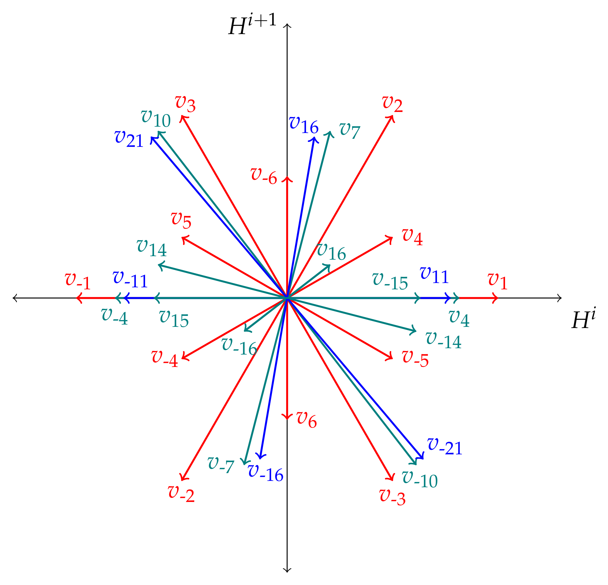
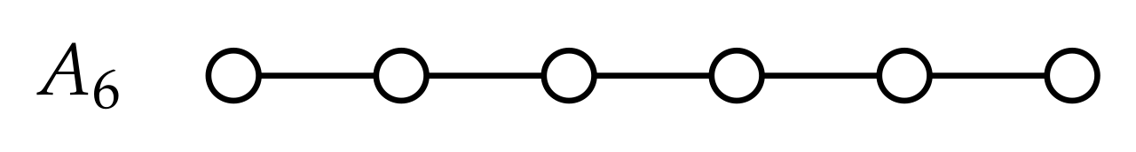
9. Roots
10. Symmetry Breaking Patterns
11. A Review of Several Example SU(7) Models
11.1. Fractionally Charged Particles and SU(7) GUT Model
11.2. Dark Matter and SU(7) GUT Model
11.3. Supersymmetry and SU(7) GUT Model
12. Conclusions
Author Contributions
Funding
Institutional Review Board Statement
Informed Consent Statement
Data Availability Statement
Acknowledgments
Conflicts of Interest
Appendix A
Appendix A.1. Generators

| SU(7) Generators | ||
|---|---|---|
Appendix A.2. Symmetric Structure Functions
| The Anti-Symmetric Structure Functions of SU(7) | |||||||||||
|---|---|---|---|---|---|---|---|---|---|---|---|
| i j k | i j k | i j k | i j k | i j k | i j k | ||||||
| 1 2 3 | 1 | 8 11 12 | 10 17 23 | 5 25 29 | 16 26 33 | 1 36 39 | |||||
| -2- | 8 13 14 | 11 18 23 | 5 26 30 | 17 25 33 | 1 37 38 | ||||||
| 1 4 7 | 9 10 15 | 11 19 22 | 6 27 30 | 17 26 34 | 2 36 38 | ||||||
| 1 5 6 | 11 12 15 | 12 18 22 | 6 28 29 | 18 27 34 | 2 37 39 | ||||||
| 2 4 6 | 13 14 15 | 12 19 23 | 7 27 29 | 18 28 33 | 3 36 37 | ||||||
| 2 5 7 | -4- | 13 20 23 | 7 28 30 | 19 27 33 | 3 38 39 | ||||||
| 3 4 5 | 1 16 19 | 13 21 22 | 8 25 26 | 19 28 34 | 4 36 41 | ||||||
| 3 6 7 | 1 17 18 | 14 20 22 | 8 27 28 | 20 29 34 | 4 37 40 | ||||||
| 4 5 8 | 2 16 18 | 14 21 23 | 8 29 30 | 20 30 33 | 5 36 40 | ||||||
| 6 7 8 | 2 17 19 | 15 16 17 | 9 25 32 | 21 29 33 | 5 37 41 | ||||||
| -3- | 3 16 17 | 15 18 19 | 9 26 31 | 21 30 34 | 6 38 41 | ||||||
| 1 9 12 | 3 18 19 | 15 20 21 | 10 25 31 | 22 31 34 | 6 39 40 | ||||||
| 1 10 11 | 4 16 21 | 15 22 23 | 10 26 32 | 22 32 33 | 7 38 40 | ||||||
| 2 9 11 | 4 17 20 | 16 17 24 | 11 27 32 | 23 31 33 | 7 39 41 | ||||||
| 2 10 12 | 5 16 20 | 18 19 24 | 11 28 31 | 23 32 34 | 8 36 37 | ||||||
| 3 9 10 | 5 17 21 | 20 21 24 | 12 27 31 | 24 25 26 | 8 38 39 | ||||||
| 3 11 12 | 6 18 21 | 22 23 24 | 12 28 32 | 24 27 28 | 8 40 41 | ||||||
| 4 9 14 | 6 19 20 | -5- | 13 29 32 | 24 29 30 | 9 36 43 | ||||||
| 4 10 13 | 7 18 20 | 1 25 28 | 13 30 31 | 24 31 32 | 9 37 42 | ||||||
| 5 9 13 | 7 19 21 | 1 26 27 | 14 29 31 | 24 33 34 | 10 36 42 | ||||||
| 5 10 14 | 8 16 17 | 2 25 27 | 14 30 32 | 25 26 35 | 10 37 43 | ||||||
| 6 11 14 | 8 18 19 | 2 26 28 | 15 25 26 | 27 28 35 | 11 38 43 | ||||||
| 6 12 13 | 8 20 21 | 3 25 26 | 15 27 28 | 29 30 35 | 11 39 42 | ||||||
| 7 11 13 | 9 16 23 | 3 27 28 | 15 29 30 | 31 32 35 | 12 38 42 | ||||||
| 7 12 14 | 9 17 22 | 4 25 30 | 15 31 32 | 33 34 35 | 12 39 43 | ||||||
| 8 9 10 | 10 16 22 | 4 26 29 | 16 25 34 | -6- | 13 40 43 | ||||||
| 13 41 42 | 18 38 45 | 23 43 45 | 27 39 46 | 33 44 47 | 38 39 48 | ||||||
| 14 40 42 | 18 39 44 | 24 36 37 | 28 38 46 | 33 45 46 | 40 41 48 | ||||||
| 14 41 43 | 19 38 44 | 24 38 39 | 28 39 47 | 34 44 46 | 42 43 48 | ||||||
| 15 36 37 | 19 39 45 | 24 40 41 | 29 40 47 | 34 45 47 | 44 45 48 | ||||||
| 15 38 39 | 20 40 45 | 24 42 43 | 29 41 46 | 35 36 37 | 46 47 48 | ||||||
| 15 40 41 | 20 41 44 | 24 44 45 | 30 40 46 | 35 38 39 | -7- | ||||||
| 15 42 43 | 21 40 44 | 25 36 47 | 30 41 47 | 35 40 41 | |||||||
| 16 36 45 | 21 41 45 | 25 37 46 | 31 42 47 | 35 42 43 | |||||||
| 16 37 44 | 22 42 45 | 26 36 46 | 31 43 46 | 35 44 45 | |||||||
| 17 36 44 | 22 43 44 | 26 37 47 | 32 42 46 | 35 46 47 | |||||||
| 17 37 45 | 23 42 44 | 27 38 47 | 32 43 47 | 36 37 48 | |||||||
Appendix A.3. Raising and Lowering Operators
| Raising Operators | ||
| Lowering Operators | ||
Appendix A.4. Positive and Simple Roots
| Positive Roots | |
| Simple Roots | |
Appendix A.5. Cartan Generators
| Cartan Generators | |
|---|---|
References
- Glashow, S.L. Partial-symmetries of weak interactions. Nucl. Phys. 1961, 22, 579–588. [Google Scholar] [CrossRef]
- Gross, D.J.; Wilczek, F. Ultraviolet Behavior of Non-Abelian Gauge Theories. Phys. Rev. Lett. 1973, 30, 1343–1346. [Google Scholar] [CrossRef] [Green Version]
- Salam, A.; Ward, J.C. Electromagnetic and weak interactions. Phys. Lett. 1964, 13, 168–171. [Google Scholar] [CrossRef]
- Salam, A. Weak and Electromagnetic Interactions. Conf. Proc. C 1968, 680519, 367–377. [Google Scholar] [CrossRef]
- Weinberg, S. A Model of Leptons. Phys. Rev. Lett. 1967, 19, 1264–1266. [Google Scholar] [CrossRef]
- Weinberg, S. Non-Abelian Gauge Theories of the Strong Interactions. Phys. Rev. Lett. 1973, 31, 494–497. [Google Scholar] [CrossRef] [Green Version]
- Yang, C.N.; Mills, R.L. Conservation of Isotopic Spin and Isotopic Gauge Invariance. Phys. Rev. 1954, 96, 191–195. [Google Scholar] [CrossRef]
- Prescott, C.; Atwood, W.B.; Cottrell, R.L.A.; Destaebler, H.; Garwin, E.L.; Gonidec, A.; Miller, R.H.; Rochester, L.S.; Sato, T.; Sherden, D.J.; et al. Parity Nonconservation in Inelastic Electron Scattering. Phys. Lett. B 1978, 77, 347–352. [Google Scholar] [CrossRef]
- Prescott, C.; Atwood, W.; Cottrell, R.; DeStaebler, H.; Garwin, E.L.; Gonidec, A.; Miller, R.; Rochester, L.; Sato, T.; Sherden, D.; et al. Further measurements of parity non-conservation in inelastic electron scattering. Phys. Lett. B 1979, 84, 524–528. [Google Scholar] [CrossRef]
- Hasert, F.; Kabe, S.; Krenz, W.; Von Krogh, J.; Lanske, D.; Morfin, J.; Schultze, K.; Weerts, H.; Bertrand-Coremans, G.; Sacton, J.; et al. Observation of Neutrino Like Interactions without Muon or Electron in the Gargamelle Neutrino Experiment. Phys. Lett. B 1973, 46, 138–140. [Google Scholar] [CrossRef]
- Hasert, F.J.; Faissner, H.; Krenz, W.; Von Krogh, J.; Lanske, D. Search for elastic muon neutrino electron scattering. Phys. Lett. B 1973, 46, 121–124. [Google Scholar] [CrossRef]
- Aad, G.; Abajyan, T.; Abbott, B.; Abdallah, J.; Khalek, S.A.; Abdelalim, A.A.; Abdinov, O.; Aben, R.; Abi, B.; Abolins, M.; et al. Observation of a new particle in the search for the Standard Model Higgs boson with the ATLAS detector at the LHC. Phys. Lett. B 2012, 716, 1–29. [Google Scholar] [CrossRef]
- Aad, G.; Abajyan, T.; Abbott, B.; Abdallah, J.; Abdel Khalek, S.; Abdinov, O.; Aben, R.; Abi, B.; Abolins, M.; AbouZeid, O.S.; et al. Measurements of Higgs boson production and couplings in diboson final states with the ATLAS detector at the LHC. Phys. Lett. B 2013, 726, 88–119. [Google Scholar] [CrossRef] [Green Version]
- Georgi, H.; Glashow, S.L. Unity of All Elementary Particle Forces. Phys. Rev. Lett. 1974, 32, 438–441. [Google Scholar] [CrossRef] [Green Version]
- Pati, J.C.; Salam, A. Lepton Number as the Fourth Color. Phys. Rev. D 1974, 10, 275–289. [Google Scholar] [CrossRef] [Green Version]
- Langacker, P. Grand Unified Theories and Proton Decay. Phys. Rept. 1981, 72, 185. [Google Scholar] [CrossRef]
- Slansky, R. Group Theory for Unified Model Building. Phys. Rept. 1981, 79, 1–128. [Google Scholar] [CrossRef]
- Dimopoulos, S.; Raby, S.; Wilczek, F. Supersymmetry and the Scale of Unification. Phys. Rev. D 1981, 24, 1681–1683. [Google Scholar] [CrossRef]
- Guth, A.H. Inflationary universe: A possible solution to the horizon and flatness problems. Phys. Rev. D 1981, 23, 347–356. [Google Scholar] [CrossRef] [Green Version]
- Linde, A. A new inflationary universe scenario: A possible solution of the horizon, flatness, homogeneity, isotropy and primordial monopole problems. Phys. Lett. B 1982, 108, 389–393. [Google Scholar] [CrossRef]
- Albrecht, A.; Steinhardt, P.J. Cosmology for Grand Unified Theories with Radiatively Induced Symmetry Breaking. Phys. Rev. Lett. 1982, 48, 1220–1223. [Google Scholar] [CrossRef]
- Efstathiou, G.P.; Ellis, R.S.; Gunn, J.E.; York, D.; Turner, M.S. Large-scale structure from quantum fluctuations in the early universe. Philos. Trans. R. Soc. Lond. Ser. A Math. Phys. Eng. Sci. 1999, 357, 7–20. [Google Scholar] [CrossRef] [Green Version]
- Dvali, G.; Shafi, Q.; Schaefer, R. Large Scale Structure and Supersymmetric Inflation without Fine Tuning. Phys. Rev. Lett. 1994, 73, 1886–1889. [Google Scholar] [CrossRef] [PubMed]
- Salopek, D.S.; Bond, J.R.; Bardeen, J.M. Designing density fluctuation spectra in inflation. Phys. Rev. D 1989, 40, 1753–1788. [Google Scholar] [CrossRef] [PubMed]
- Di Marco, A.; Pradisi, G.; Cabella, P. Inflationary scale, reheating scale, and pre-BBN cosmology with scalar fields. Phys. Rev. D 2018, 98, 123511. [Google Scholar] [CrossRef] [Green Version]
- Kolb, E.W.; Linde, A.; Riotto, A. Grand-Unified-Theory Baryogenesis after Preheating. Phys. Rev. Lett. 1996, 77, 4290–4293. [Google Scholar] [CrossRef] [Green Version]
- Kofman, L.; Linde, A.; Starobinsky, A.A. Reheating after Inflation. Phys. Rev. Lett. 1994, 73, 3195–3198. [Google Scholar] [CrossRef] [Green Version]
- Felder, G.N.; Kofman, L.; Linde, A.D. Instant preheating. Phys. Rev. D 1999, 59, 123523. [Google Scholar] [CrossRef] [Green Version]
- Rangarajan, R.; Nanopoulos, D.V. Inflationary baryogenesis. Phys. Rev. D 2001, 64, 063511. [Google Scholar] [CrossRef] [Green Version]
- Kim, J.E. Flavor unity in SU (7): Low-mass magnetic monopole, doubly charged lepton, and Q= 5 3,- 4 3 quarks. Phys. Rev. D 1981, 23, 2706. [Google Scholar] [CrossRef]
- Farhi, E.; Susskind, L. A TECHNICOLORED G.U.T. Phys. Rev. D 1979, 20, 202. [Google Scholar]
- Farhi, E.; Susskind, L. Technicolour. Phys. Rep. 1981, 74, 277–321. [Google Scholar] [CrossRef] [Green Version]
- Kuang, Y.P.; Tye, S.H. Grand unification with a confining model of the weak interactions. Phys. Rev. D 1982, 26, 1718. [Google Scholar] [CrossRef]
- Chávez, H.; Martins Simões, J.A. The muon g-2 in an SU(7) left right symmetric model with mirror fermions. Nucl. Phys. B 2007, 783, 76–89. [Google Scholar] [CrossRef] [Green Version]
- Diaz, R.A.; Gallego, D.; Martinez, R. Renormalization Group and Grand Unification with 331 Models. Int. J. Mod. Phys. A 2007, 22, 1849–1874. [Google Scholar] [CrossRef] [Green Version]
- Brümmer, F.; Fichet, S.; Hebecker, A.; Kraml, S. Phenomenology of supersymmetric Gauge-Higgs unification. J. High Energy Phys. 2009, 2009, 011. [Google Scholar] [CrossRef] [Green Version]
- Barr, S.M. Doubly lopsided mass matrices from supersymmetric SU(N) unification. Phys. Rev. D 2008, 78, 055008. [Google Scholar] [CrossRef] [Green Version]
- Goetz, A.; Secrest, J.A. The algebraic structure of the SU(7) Lie group. J. Math. Phys. 2019, 60, 101703. [Google Scholar] [CrossRef]
- Group, P.D. Review of Particle Physics. Prog. Theor. Exp. Phys. 2020, 2020, 083C01. Available online: https://academic.oup.com/ptep/article-pdf/2020/8/083C01/34673722/ptaa104.pdf (accessed on 5 April 2021). [CrossRef]
- Pauli, W., Jr. Zur Quantenmechanik des magnetischen Elektrons. (On the quantum mechanics of the magnetic electron). Z. Phys. 1927, 43, 601–623. (In German) [Google Scholar] [CrossRef]
- Gell-Mann, M. Symmetries of Baryons and Mesons. Phys. Rev. 1962, 125, 1067–1084. [Google Scholar] [CrossRef] [Green Version]
- Einstein, A. Die Grundlage der allgemeinen Relativitätstheorie. Ann. Phys. 1916, 354, 769–822. [Google Scholar] [CrossRef] [Green Version]
- Umemura, I.; Yamamoto, K. A Symmetry Breaking Pattern in the SU(7) Grand Unified Model. Prog. Theor. Phys. 1981, 66, 1430–1447. [Google Scholar] [CrossRef] [Green Version]
- Feger, R.; Kephart, T.W.; Saskowski, R.J. LieART 2.0—A Mathematica application for Lie Algebras and Representation Theory. Comput. Phys. Commun. 2020, 257, 107490. [Google Scholar] [CrossRef]
- Higgs, P.W. Broken symmetries, massless particles and gauge fields. Phys. Lett. 1964, 12, 132–133. [Google Scholar] [CrossRef]
- Higgs, P.W. Broken Symmetries and the Masses of Gauge Bosons. Phys. Rev. Lett. 1964, 13, 508–509. [Google Scholar] [CrossRef] [Green Version]
- Higgs, P.W. Spontaneous Symmetry Breakdown without Massless Bosons. Phys. Rev. 1966, 145, 1156–1163. [Google Scholar] [CrossRef] [Green Version]
- Englert, F.; Brout, R. Broken Symmetry and the Mass of Gauge Vector Mesons. Phys. Rev. Lett. 1964, 13, 321–323. [Google Scholar] [CrossRef] [Green Version]
- Guralnik, G.S.; Hagen, C.R.; Kibble, T.W.B. Global Conservation Laws and Massless Particles. Phys. Rev. Lett. 1964, 13, 585–587. [Google Scholar] [CrossRef] [Green Version]
- Li, L.F.; Wilczek, F. Price of fractionally charged particles in a unified model. Phys. Lett. B 1981, 107, 64–68. [Google Scholar] [CrossRef]
- Nakano, T.; Nishijima, K. Charge Independence for V-particles. Prog. Theor. Phys. 1953, 10, 581–582. [Google Scholar] [CrossRef] [Green Version]
- Nishijima, K. Charge Independence Theory of V Particles. Prog. Theor. Phys. 1955, 13, 285–304. [Google Scholar] [CrossRef] [Green Version]
- Gell-Mann, M. The interpretation of the new particles as displaced charge multiplets. Nuovo Cim. 1956, 4, 848–866. [Google Scholar] [CrossRef]
- Ma, E. Unified framework for matter, dark matter, and radiative neutrino mass. Phys. Rev. D 2013, 88, 117702. [Google Scholar] [CrossRef] [Green Version]
- Callen, B.D.; Volkas, R.R. Clash-of-symmetries mechanism from intersecting domain-wall branes. Phys. Rev. D 2014, 89, 056004. [Google Scholar] [CrossRef] [Green Version]
- Callen, B.D. Unified Dark Matter from a Simple Gauge Group on a Domain-Wall Brane. arXiv 2017, arXiv:1705.02086. [Google Scholar]
- Frampton, P.H.; Kephart, T.W. Fractionally Charged Particles as Evidence for Supersymmetry. Phys. Rev. Lett. 1982, 49, 1310–1313. [Google Scholar] [CrossRef]
- Kubo, J.; Sakakibara, S. Spontaneous gauge symmetry breaking in nonminimal supersymmetric grand unified theories. J. Phys. G Nucl. Phys. 1983, 9, 475–496. [Google Scholar] [CrossRef]
- Amato, A.; Bali, G.; Lucini, B. Topology and glueballs in SU(7) Yang-Mills with open boundary conditions. arXiv 2015, arXiv:1512.00806. [Google Scholar]
- DeGrand, T.; Liu, Y.; Neil, E.T.; Shamir, Y.; Svetitsky, B. Spectroscopy of SU(4) gauge theory with two flavors of sextet fermions. Phys. Rev. D 2015, 91, 114502. [Google Scholar] [CrossRef] [Green Version]
- Bali, G.; Bursa, F.; Castagnini, L.; Collins, S.; Del Debbio, L.; Lucini, B.; Panero, M. Mesons in large-N QCD. J. High Energy Phys. 2013, 2013. [Google Scholar] [CrossRef] [Green Version]
- Lucini, B.; Rago, A.; Rinaldi, E. SU(Nc) gauge theories at deconfinement. Phys. Lett. B 2012, 712, 279–283. [Google Scholar] [CrossRef] [Green Version]
- Racah, G. Theory of Complex Spectra. IV. Phys. Rev. 1949, 76, 1352–1365. [Google Scholar] [CrossRef]
- Judd, B. Lie groups for atomic shells. Phys. Rep. 1997, 285, 1–76. [Google Scholar] [CrossRef]
- Judd, B.R.; Lister, G.M.S. Complementary groups in the quark model of the atom. J. Phys. A Math. Gen. 1992, 25, 2615–2630. [Google Scholar] [CrossRef]


Publisher’s Note: MDPI stays neutral with regard to jurisdictional claims in published maps and institutional affiliations. |
© 2021 by the authors. Licensee MDPI, Basel, Switzerland. This article is an open access article distributed under the terms and conditions of the Creative Commons Attribution (CC BY) license (https://creativecommons.org/licenses/by/4.0/).
Share and Cite
Jones, D.; Secrest, J.A. Construction and Characterization of Representations of SU(7) for GUT Model Builders. Symmetry 2021, 13, 1044. https://doi.org/10.3390/sym13061044
Jones D, Secrest JA. Construction and Characterization of Representations of SU(7) for GUT Model Builders. Symmetry. 2021; 13(6):1044. https://doi.org/10.3390/sym13061044
Chicago/Turabian StyleJones, Daniel, and Jeffery A. Secrest. 2021. "Construction and Characterization of Representations of SU(7) for GUT Model Builders" Symmetry 13, no. 6: 1044. https://doi.org/10.3390/sym13061044