Article

Pareto Optimality for Multioptimization of Continuous Linear Operators

by
Clemente Cobos-Sánchez
1,*,†,
José Antonio Vilchez-Membrilla
1,†,
Almudena Campos-Jiménez
2,† and
Francisco Javier García-Pacheco
2,†
1
Department of Electronics, College of Engineering, University of Cadiz, 11510 Puerto Real, Spain
2
Department of Mathematics, College of Engineering, University of Cadiz, 11510 Puerto Real, Spain
*
Author to whom correspondence should be addressed.
These authors contributed equally to this work.
Symmetry 2021, 13(4), 661; https://doi.org/10.3390/sym13040661
Submission received: 11 March 2021 / Revised: 29 March 2021 / Accepted: 8 April 2021 / Published: 12 April 2021

Abstract

:
This manuscript determines the set of Pareto optimal solutions of certain multiobjective-optimization problems involving continuous linear operators defined on Banach spaces and Hilbert spaces. These multioptimization problems typically arise in engineering. In order to accomplish our goals, we first characterize, in an abstract setting, the set of Pareto optimal solutions of any multiobjective optimization problem. We then provide sufficient topological conditions to ensure the existence of Pareto optimal solutions. Next, we determine the Pareto optimal solutions of convex max–min problems involving continuous linear operators defined on Banach spaces. We prove that the set of Pareto optimal solutions of a convex max–min of form max T ( x ) , min x coincides with the set of multiples of supporting vectors of T. Lastly, we apply this result to convex max–min problems in the Hilbert space setting, which also applies to convex max–min problems that arise in the design of truly optimal coils in engineering.

1. Introduction

Multiobjective optimization problems (MOPs) appear quite often in all areas of pure and applied mathematics, for instance, in the geometry of Banach spaces [1,2,3], in operator theory [4,5,6,7], in lineability theory [8,9,10], in differential geometry [11,12,13,14], and in all areas of Experimental, Medical and Social Sciences [15,16,17,18,19,20]. By means of MOPs, many real-life situations can be modeled accurately. However, the existence of a global solution that optimizes all the objective functions of an MOP at once is very unlikely. This is were Pareto optimal solutions (POS) come into play. Informally speaking, a POS is a feasible solution such that, if any other feasible solution is more optimal at one objective function, then it is less optimal at another objective function. Pareto optimal solutions are sometimes graphically displayed in Pareto charts (PC). In this manuscript, we prove a characterization of POS by relying on orderings and equivalence relations. We also provide a sufficient topological condition to guarantee the existence of Pareto optimal solutions.
This work is mainly motivated by certain MOPs appearing in engineering, such as the design of truly optimal transcranial magnetic stimulation (TMS) coils [18,19,20,21,22,23]. The main goal of this manuscript is to characterize (Theorem 6) the set of Pareto optimal solutions of the MOPs that appear in the design of coils, such as (3). In the case of MOPs in which operators are defined on Hilbert spaces, this characterization is improved (Corollary 1). Under this Hilbert space setting, we also study the relationships between different MOPs involving different operators, but which are defined on the same Hilbert space. These operators can be naturally combined to obtain a new MOP. The set of Pareto optimal solutions of this new MOP is compared (Corollary 2) to the set of Pareto optimal solutions of the initial MOPs.

2. Materials and Methods

In this section, we compile all necessary tools to accomplish our results. We also develop new and original tools, such as Theorem 1 and Corollary 2, which contribute to enriching the literature on optimization theory.

2.1. Formal Description of MOPs

A generic multiobjective optimization problem (MOP) has the following form:
M : = max f i ( x ) i = 1 , , p , min g j ( x ) j = 1 , , q , x R ,
where f i , g j : X R are called objective functions, defined on a nonempty set X, and R is a nonempty subset of X called the feasible region or region of constraints/restrictions. The set of general solutions of the above MOP is denoted by sol ( M ) . In fact,
sol ( M ) : = { x R : y R i { 1 , , p } j { 1 , , q } f i ( x ) f i ( y ) , g j ( x ) g j ( y ) } .
It is obvious that
sol ( M ) = sol ( P 1 ) sol ( P p ) sol ( Q 1 ) sol ( Q q )
where
P i : = max f i ( x ) , x R , and Q j : = min g j ( x ) , x R ,
are single-objective optimization problems (SOPs) and sol ( P i ) , sol ( Q j ) denote the set of general solutions of P i , Q j for i = 1 , , p and j = 1 , , q , respectively. The set of Pareto optimal solutions of MOP M is defined as
Pos ( M ) : = { x R : y R , if there exists i { 1 , , p } with f i ( y ) > f i ( x ) or j { 1 , , q } with g j ( y ) < g j ( x ) , then there exists i { 1 , , p } with f i ( y ) < f i ( x ) or j { 1 , , q } with g j ( x ) < g j ( y ) } .
To guarantee the existence of general solutions, it is usually asked for X to be a Hausdorff topological space, R is a compact subset of X, f i s are upper semicontinuous, and g j s are lower semicontinuous. This way, at least we make sure that the SOPs P i s and Q j s have at least one solution (Weierstrass extreme value theorem). Even more, solution sets sol ( P i ) and sol ( Q j ) are closed and thus compact, which makes sol ( M ) also compact. Nevertheless, even under these conditions, sol ( M ) might still be empty, as we can easily infer from Equation (2).

2.2. Characterizing Pareto Optimal Solutions

A more abstract way to construct the set of Pareto optimal solutions follows. Let X be a nonempty set, f i , g j : X R functions and R a nonempty subset of X. In R , consider the equivalence relation given by
S : = ( x , y ) R 2 : i = 1 , , p j = 1 , , q f i ( x ) = f i ( y ) , g j ( x ) = g j ( y ) .
Next, in the quotient set of R by S , R S , consider the order relation given by
[ x ] S [ y ] S i = 1 , , p j = 1 , , q f i ( x ) f i ( y ) , g j ( y ) g j ( x ) .
Theorem 1. 
Consider MOP (1). Then,
Pos ( M ) = x R : [ x ] S i s a m a x i m a l e l e m e n t o f R S e n d o w e d w i t h
and
sol ( M ) : = x R : [ x ] S i s t h e m a x i m u m o f R S e n d o w e d w i t h .
As a consequence, sol ( M ) Pos ( M ) . If there exists i 1 { 1 , , p } or j 1 { 1 , , q } such that sol ( P i 1 ) or sol ( Q j 1 ) is a singleton, respectively, then sol ( P i 1 ) Pos ( M ) or sol ( Q j 1 ) Pos ( M ) , respectively.
Proof. 
Fix an arbitrary x 0 Pos ( M ) . Let us assume that there is y R , so that [ x 0 ] S < [ y ] S . Then, f i ( x 0 ) f i ( y ) for all i = 1 , , p and g j ( x 0 ) g j ( y ) for all j = 1 , , q . However, [ x 0 ] S [ y ] S ; therefore, there exists i 0 { 1 , , p } or j 0 { 1 , , q } such that f i 0 ( x 0 ) < f i 0 ( y ) or g j 0 ( x 0 ) < g j 0 ( y ) , respectively. Since x 0 Pos ( M ) by assumption, there exists i 1 { 1 , , p } or j 1 { 1 , , q } , such that f i 1 ( x 0 ) > f i 1 ( y ) or g j 1 ( x 0 ) < g j 1 ( y ) , respectively, which is a contradiction. Therefore, [ x 0 ] S is a maximal element of R S endowed with ≤. The arbitrariness of x 0 Pos ( M ) shows that
Pos ( M ) x R : [ x ] S i s a maximal element of R S endowed with .
Conversely, fix an arbitrary x 0 R , such that [ x 0 ] S is a maximal element of R S endowed with ≤. Take y R satisfying that there exists i 0 { 1 , , p } or j 0 { 1 , , q } with f i 0 ( y ) > f i 0 ( x 0 ) or g j 0 ( y ) < g j 0 ( x 0 ) , respectively. If f i ( x 0 ) f i ( y ) for all i { 1 , , p } { i 0 } and g j ( x 0 ) g j ( y ) for all j { 1 , , q } { j 0 } , then [ x 0 ] S < [ y ] S , reaching a contradiction with the maximality of [ x 0 ] S in R S endowed with ≤. This shows that
Pos ( M ) = x R : [ x ] S is a maximal element of R S endowed with .
Next, fix an arbitrary x 0 sol ( M ) . For every y R , f i ( x 0 ) f i ( y ) and g j ( x 0 ) g j ( y ) for all i = 1 , , p and all j = 1 , , q . Then, [ x 0 ] S [ y ] S . The arbitrariness of y R ensures that [ x 0 ] S is a maximal element of R S endowed with ≤. Conversely, fix an arbitrary x 0 R , such that [ x 0 ] S is a maximal element of R S endowed with ≤. For every y R , [ y ] S [ x 0 ] S ; therefore, f i ( x 0 ) f i ( y ) and g j ( x 0 ) g j ( y ) for all i = 1 , , p and all j = 1 , , q . The arbitrariness of y R proves that x 0 sol ( M ) . We proved that
sol ( M ) : = x R : [ x ] S is the maximum of R S endowed with .
Lastly, suppose that sol ( P i 1 ) is a singleton for some i 1 { 1 , , p } , and write sol ( P i 1 ) = { x 0 } . Take y R satisfying that there exists i 0 { 1 , , p } or j 0 { 1 , , q } with f i 0 ( y ) > f i 0 ( x 0 ) or g j 0 ( y ) < g j 0 ( x 0 ) , respectively. If such i 0 exists, then i 0 i 1 . By hypothesis, f i 1 ( x 0 ) > f i 1 ( y ) since y sol ( P i 1 ) . This shows that x 0 Pos ( M ) . Likewise, sol ( Q j 1 ) Pos ( M ) provides that sol ( Q j 1 ) is a singleton. □
Lemma 1. 
Consider MOP (1). Let i 0 { 1 , , p } , j 0 { 1 , , q } . Then,
1. 
If there is x i 0 R so that x i 0 S is a maximal element of [ x ] S : x arg max R f i 0 , then x i 0 S is a maximal element of R / S . Hence, x i 0 Pos ( M ) .
2. 
If there is x j 0 R so that x j 0 S is a maximal element of [ x ] S : x arg min R g j 0 , then x j 0 S is a maximal element of R / S . Hence, x j 0 Pos ( M )
Proof. 
We only prove the first item since the other follows a dual proof. Assume that x i 0 S is not a maximal element of R / S . Then, we can find y R in such a way that x i 0 S < [ y ] S . In particular, f i 0 x i 0 f i 0 ( y ) ; therefore, f i 0 ( y ) = max R f i 0 ; hence, y arg max R f i 0 . As a consequence, [ y ] S [ x ] S : x arg max R f i 0 , contradicting that x i 0 S be a maximal element of [ x ] S : x arg max R f i 0 . □
Theorem 2. 
Consider MOP (1). If X is a topological space, R is a compact Hausdorff subset of X and all the objective functions are continuous, then Pos ( M ) .
Proof. 
Fix i 0 { 1 , , p } . In accordance with Lemma 1, it is only sufficient to find a maximal element of A : = [ x ] S : x arg max R f i 0 . We rely on Zorn’s lemma. Consider a chain in A, that is, a totally ordered subset of elements [ x k ] S , with k ranging a totally ordered set K in such a way that k 1 < k 2 if and only if x k 1 S < x k 2 S . Since K is totally ordered, we have that x k k K is a net in R . The compactness of R allows for extracting a subnet ( y h ) h H of x k k K convergent to some x 0 R . Let us first show that x 0 arg max R f i 0 . The continuity of f i 0 implies that f i 0 ( y h ) h H converges to f i 0 ( x 0 ) . Fix any ε > 0 . There is h ε H satisfying that, if h h ε , then f i 0 ( y h ) f i 0 ( x 0 ) < ε . Fix any k 0 K . There is h 0 H , so that y h : h h 0 { x k : k k 0 } . Since H is a directed set, we can find h 1 H with h 1 h ε and h 1 h 0 . There exists k 1 K with k 1 k 0 such that y h 1 = x k 1 . Next, f i 0 y h 1 = f i 0 x k 1 = max R f i 0 . As a consequence,
max R f i 0 f ( x 0 ) = f i 0 y h 1 f ( x 0 ) < ε .
The arbitrariness of ε shows that max R f i 0 = f ( x 0 ) . Lastly, we prove that [ x 0 ] S is an upper bound for chain [ x k ] S : k K . Fix an arbitrary k 0 K . In order to prove that x k 0 S [ x 0 ] S , we have to check that f i x k 0 f i ( x 0 ) for all i { 1 , , p } and g j x k 0 g j ( x 0 ) for all j { 1 , , q } . Indeed, fix i { 1 , , p } and suppose to the contrary that f i x k 0 > f i ( x 0 ) . Let 0 < ε < f i x k 0 f i ( x 0 ) . There exists h ε H such that, if h h ε , then f i ( y h ) f i ( x 0 ) < ε . We can find h 0 H , such that y h : h h 0 { x k : k k 0 } . Since H is a directed set, we can find h 1 H with h 1 h ε and h 1 h 0 . There exists k 1 K with k 1 k 0 such that y h 1 = x k 1 . Since k 0 k 1 , we have that x k 0 S x k 1 S . Thus,
f i y h 1 = f i x k 1 f i x k 0 > f i ( x 0 ) ,
contradicting that f i y h 1 f i ( x 0 ) < ε . In a similar way, it can be shown that g j x k 0 g j ( x 0 ) for all j { 1 , , q } . As a consequence, x k 0 S [ x 0 ] S . In other words, [ x 0 ] S is an upper bound for the chain [ x k ] S : k K . Since every chain of A has an upper bound, Zorn’s lemma ensures the existence of maximal elements in A. □

2.3. MOPs in a Functional-Analysis Context

A large number of objective functions in an MOP may cause a lack of general solutions, that is, sol ( M ) = . This happens quite often with MOPs involving matrices. Even if the number of objective functions is short, we might still have sol ( M ) = . The following theorem [20], Theorem 2, is a very representative example of this situation of lack of general solutions.
Theorem 3. 
Let T : X Y be a nonzero continuous linear operator, where X , Y are normed spaces; then, the following max–min problem is free of general solutions:
max T ( x ) , min x , x X .
Equation (3) describes an MOP that appears in bioengineering quite often after the linearization of forces or fields [18].

3. Results

We focus on MOPs similar to (3). In fact, we find Pos ( 3 ) (Theorem 6 and Corollary 1). If X , Y are Hilbert spaces, say H , K , and T 1 , , T k B ( H , K ) are continuous linear operators, then the sets of Pareto optimal solutions of the MOPs
max T i ( x ) , min x , x H ,
for i = 1 , , k are compared (Corollary 2) with the set of Pareto optimal solutions of MOP
max T ( x ) , min x , x H ,
where
T : H K 2 k 2 K x T ( x ) = T 1 ( x ) , , T k ( x ) .

3.1. Formatting of Mathematical Components

Let X , Y be normed spaces. Consider a nonzero continuous linear operator T : X Y . Then
T : = sup { T ( x ) : x B X }
is the norm of T. On the other hand,
suppv ( T ) : = { x S X : T ( x ) = T } ,
stands for the set of supporting vectors of T, where B X : = { x X : x 1 } is a (closed) unit ball, and S X : = { x X : x = 1 } is the unit sphere. Continuous linear operators are also called bounded because they are bounded on the unit ball. The space of bounded linear operators from X to Y is denoted as B ( X , Y ) .
Let H be a Hilbert space, and consider the dual map of H:
J H : H H * k J H ( k ) : = k * = ( | k ) .
J H is a surjective linear isometry between H and H * (Riesz representation theorem). In the frame of the geometry of Banach spaces, J H is called duality mapping.
Consider H , K Hilbert spaces, and let T B ( H , K ) be a bounded linear operator. We define the adjoint operator of T as T : = ( J H ) 1 T * J K B ( K , H ) , with T * : K * H * as the dual operator of T. The most representative property of the adjoint operator is that it is the unique operator in B ( K , H ) satisfying ( T ( x ) | y ) = ( x | T ( y ) ) for all x H and all y K . It holds that T = T , T = T , ( T + S ) = T + S and ( λ T ) = λ ¯ T .
If T B ( H ) verifies T = T , then T is self-adjoint. This is equivalent to equality ( T ( x ) | y ) = ( x | T ( y ) ) held for every x , y H . If T satisfies ( T ( x ) | x ) 0 for each x H , then T is called positive. If H is complex, then T B ( H ) is self-adjoint if and only if ( T ( x ) | x ) R for each x H . Thus, in complex Hilbert spaces, positive operators are self-adjoint. T is strongly positive if there exists S B ( H , K ) with T = S S . Typical examples of self-adjoint positive operators are strongly positive operators.
For each T B ( H ) , the following set is the spectrum of T
σ ( T ) : = λ C : λ I T U B ( H ) ,
where U B ( H ) is the multiplicative group of invertible operators on H. Among spectral properties, it is compact, nonempty, and T max | σ ( T ) | . We work with a special subset of the spectrum:
σ p ( T ) : = λ C : ker ( λ I T ) { 0 } ,
called the point spectrum, whose elements are eigenvalues of T. It is clear that σ p ( T ) σ ( T ) . In addition, if λ σ p ( T ) , the subspace of associated eigenvectors to λ is
V ( λ ) : = x H : T ( x ) = λ x .
If T is an eigenvalue of T or, in other words, T σ p ( T ) , then T is the maximal element of | σ ( T ) | , i.e., T = max | σ ( T ) | . In this situation, we also write T = λ max ( T ) .
Example 1. 
Let T : H K be a continuous linear operator where H , K are Hilbert spaces, such that T σ p ( T ) ; then, V ( T ) S X suppv ( T ) . If x V ( T ) S X , then T ( x ) = T x ; therefore, T ( x ) = T and hence x suppv ( T ) .
In general, T σ p ( T ) , unless, for instance, T is compact, self-adjoint, and positive. This is why we have to rely on adjoint T and strongly positive operator T T . It is straightforward to verify that the eigenvalues of a positive operator are positive, and in the case of a self-adjoint operator, the eigenvalues are real. When T is compact, it holds that T T is compact, self-adjoint, and positive.
The next result was obtained by refining ([10] [Theorem 9]). In particular, we obtained the same conclusions with fewer hypotheses.
Theorem 4. 
Consider H , K Hilbert spaces, and T B ( H , K ) . Then,
1. 
T 2 = T T .
2. 
suppv ( T ) suppv T T .
3. 
supp ( T ) if and only if T T σ p T T .
In this situation, T = λ max T T and suppv ( T ) = V λ max ( T T ) S H .
Proof. 
  • Fix an element x H , and the associated mapping x * : = ( | x ) . Then,
    T ( x ) 2 = T ( x ) | T ( x ) = T ( T ( x ) ) | x = x * T T ( x )
    x * T ( T ( x ) ) x * T T x = T T x 2
    T T x 2 = T 2 x 2 .
    If element x is taken in the unit sphere, i.e., x S X , and considering the previous inequalities, we concluded that T 2 = T T .
  • Let x suppv ( T ) be an arbitrary element; then, Equation (6) implies that
    T ( T ( x ) ) = T 2 = T T ( x ) = T T ( x ) .
    Then, x suppv T T .
  • Take v suppv ( T ) . Before anything else, since suppv ( T ) suppv T T , we have that
    T T ( v ) T T = T T ( v ) T T = T T T T = 1 .
    Following chain of equalities (6),
    v * T T ( v ) T T = T ( v ) 2 T T = T 2 v 2 T T = 1 .
    Thanks to the strict convexity of space H,
    T T ( v ) T T = v ,
    that is,
    T T ( v ) = T T v
    and so T T σ p T T . We implicitly proved that suppv ( T ) V T T S H .
    Conversely, let us suppose that T T σ p T T . As we remarked before, T T is a strongly positive operator, so the eigenvalues of that operator are real and positive. Therefore, equality λ max T T = T T holds, which implies that
    T = T 2 = T T = λ max T T .
    Take w V λ max T T S H . Then
    T ( w ) 2 = w * T T ( w ) = w * λ max T T w = λ max T T = T T = T 2 .
    This chain of equalities proves that w suppv ( T ) . Consequently,
    V λ max T T S H suppv ( T ) .
 □
The following technical lemma establishes the behavior of the point spectrum of a linear combination of operators. However, we first introduce some notation. Considering bounder linear operator T B ( H , K ) defined between H and K, Hilbert spaces, then
V ( T ) : = λ σ p ( T ) V ( λ ) .
Lemma 2. 
If we consider Hilbert spaces, H , K , and T 1 , , T k B ( H , K ) , then, for every α 1 , , α k C ,
i = 1 k V ( T i ) V i = 1 k α i T i .
Proof. 
Take any x i = 1 k V ( T i ) . If x = 0 , there is nothing to prove, x is actually in V i = 1 k α i T i . So, assume that x 0 . For every i { 1 , , k } , there exists λ i σ ( T i ) , such that x V ( λ i ) , that is, T i ( x ) = λ i x . Then
i = 1 k α i T i ( x ) = i = 1 k α i T i ( x ) = i = 1 k α i λ i x = i = 1 k α i λ i x .
This shows that
x V i = 1 k α i λ i V i = 1 k α i T i .
 □
The hypothesis in Lemma 3 is, in fact, very restrictive.
Lemma 3. 
If H , K are Hilbert spaces, and T 1 , , T k B ( H , K ) , such that V ( T i ) ker ( T i ) ker ( T j ) for all i , j { 1 , , k } with i j . For every i { 1 , , k } and every x i V ( T i ) ker ( T i ) , there are α 1 , , α k C , such that
i = 1 k β i x i V i = 1 k α i T i
for every β 1 , , β k C .
Proof. 
For every i { 1 , , k } , there exists λ i σ ( T i ) { 0 } , such that x i V ( λ i ) , that is, T i ( x i ) = λ i x i . Define α i : = λ i 1 for every i { 1 , , k } . Then
i = 1 k α i T i i = 1 k β i x i = i = 1 k α i β i T i ( x i ) = i = 1 k α i β i λ i x i = i = 1 k β i x i .
 □
If H 1 , , H p are Hilbert spaces, then i = 1 p H i 2 is a Hilbert space, considering the following scalar product and norm
( h i ) i = 1 p ( k i ) i = 1 p : = i = 1 p ( h i | k i ) , ( h i ) i = 1 p : = i = 1 p h i 2 ,
for all ( h i ) i = 1 p , ( k i ) i = 1 p i = 1 p H i 2 . If H is another Hilbert space and T i : H H i is a continuous linear operator for each i = 1 , , p , then the direct sum of T 1 , , T p is defined as
i = 1 p T i 2 : H i = 1 p H i 2 x i = 1 p T i 2 ( x ) : = T i ( x ) i = 1 p .
If S i : H i H is a continuous linear operator for each i = 1 , , p , then the direct sum of S 1 , , S p is now defined as
i = 1 p S i 2 : i = 1 p H i 2 H ( h i ) i = 1 p i = 1 p S i 2 ( h i ) i = 1 p : = i = 1 p S i ( h i ) .
Theorem 5. 
Suppose that H , H 1 , , H p are Hilbert spaces, and let T i : H H i be a continuous linear operator for each i = 1 , , p . Then, i = 1 p T i 2 = i = 1 p T i 2 and
i = 1 p T i 2 i = 1 p T i 2 = i = 1 p T i T i .
Proof. 
Fix arbitrary elements x H and ( h i ) i = 1 p i = 1 p H i 2 . Then,
x i = 1 p T i 2 ( h i ) i = 1 p = x | i = 1 p T i ( h i ) = i = 1 p x | T i ( h i ) = i = 1 p T i ( x ) | h i = T i ( x ) i = 1 p | ( h i ) i = 1 p = i = 1 p T i 2 ( x ) | ( h i ) i = 1 p .
Lastly, for each x H ,
i = 1 p T i 2 i = 1 p T i 2 ( x ) = i = 1 p T i 2 i = 1 p T i 2 ( x ) = i = 1 p T i 2 T i ( x ) i = 1 p = i = 1 p T i T i ( x ) = i = 1 p T i T i ( x ) .
 □

3.2. Pareto Optimal Solutions of the MOP max T ( x ) , min x , x X

Under the settings of Theorem 3, arg min x X x = { 0 } ; therefore, in view of Theorem 1, 0 Pos ( 3 ) . This Pareto optimal solution is usually disregarded when it comes to a real-life problem.
Theorem 6. 
Let X , Y be normed spaces, and T : X Y be a nonzero continuous linear operator. Then, Pos ( 3 ) = R suppv ( T ) .
Proof. 
Fix an arbitrary x 0 Pos ( 3 ) . Since x 0 = x 0 x 0 x 0 , it is sufficient if we show that x 0 x 0 suppv ( T ) . Therefore, we may assume that x 0 = 1 , so our aim was summed up to prove that T ( x 0 ) = T . Since x 0 S X B X , T ( x 0 ) T . Suppose that T ( x 0 ) < T . By the definition of sup, there exists y B X , such that T ( x 0 ) < T ( y ) T . y 1 = x 0 and T ( x 0 ) < T ( y ) , which contradicts that x 0 Pos ( 3 ) . As a consequence, T ( x 0 ) = T ; hence, x 0 suppv ( T ) . The arbitrariness of x 0 Pos ( 3 ) shows that Pos ( 3 ) R suppv ( T ) . Conversely, fix an arbitrary x 0 R suppv ( T ) . There exists y 0 suppv ( T ) and α R , such that x 0 = α y 0 . Observe that x 0 = | α | y 0 = | α | . We prove that x 0 Pos ( 3 ) . Let us consider an element y X satisfying that y < x 0 = | α | , and we distinguish cases: if y = 0 , then T ( x 0 ) = | α | T ( y 0 ) = | α | T > 0 = T ( y ) . If y 0 , then
T ( x 0 ) = | α | T ( y 0 ) = | α | T | α | T y y > T ( y ) .
Lastly, if there exists y X , such that T ( y ) > T ( x 0 ) , then
| α | T = T ( x 0 ) < T ( y ) T y ,
which means that x 0 = | α | < y . □
When X , Y are Hilbert spaces, the Pareto optimal solutions of (3) are directly obtained via combining Theorems 4 and 6.
Corollary 1. 
Let T : H K be a continuous linear operator with H , K Hilbert spaces. Then, Pos ( 3 ) = V λ max T T .
This last result allows for solving the following MOP (motivated in Section 4), given by
max T 1 ( x ) 2 + + T k ( x ) 2 , min x , x H .
The Pareto optimal solutions of (11) are related to those of
max T i ( x ) , min x , x H ,
for i = 1 , , k .
Corollary 2. 
If T 1 , , T k B ( H , K ) are continuous linear operators between Hilbert spaces H and K, then:
1. 
Pos ( 11 ) = V λ max i = 1 k T i T i .
2. 
i = 1 k Pos ( 12 ) Pos ( 11 ) .
Proof. 
Consider bounded linear operator
T 1 2 k 2 T k : H K 2 k 2 K x T 1 2 k 2 T k ( x ) : = T 1 ( x ) , , T k ( x ) .
The next equality trivially holds for every x H ,
T 1 ( x ) , , T k ( x ) 2 = T 1 ( x ) 2 + + T k ( x ) 2 .
Since the square root is strictly increasing, (11) is equivalent to
max T 1 2 k 2 T k ( x ) , min x , x H ,
which is an MOP of form (3).
  • According to Corollary 1 and Theorem 5,
    Pos ( 11 ) = Pos ( 13 ) = V λ max T 1 2 k 2 T k T 1 2 k 2 T k = V λ max i = 1 k T i T i .
  • We rely on Theorem 6 and Corollary 1. Fix an arbitrary x i = 1 k Pos ( 12 ) . If x = 0 , then x R suppv T 1 2 k 2 T k = Pos ( 13 ) = Pos ( 11 ) . Suppose that x 0 . In view of Theorem 6, x x i = 1 k suppv ( T i ) . We prove that x x suppv T 1 2 k 2 T k . Take any y B H . Since x x i = 1 k suppv ( T i ) , for every i { 1 , , k } ,
    T i x x T i ( y ) .
    As a consequence,
    T 1 2 k 2 T k x x = T 1 x x 2 + + T k x x 2 T 1 y 2 + + T k y 2 = T 1 2 k 2 T k y .
    This means that x x suppv T 1 2 k 2 T k . In accordance with Theorem 6,
    x = x x x R suppv T 1 2 k 2 T k = Pos ( 13 ) = Pos ( 11 ) .
 □

4. Discussion

In order to design truly optimal TMS coils, and depending on the nature and characteristics of the coil that we want to maximize or minimize, a linearization technique is applied to the electromagnetic field [18,23,24,25]; then, MOPs like (3) come out:
max E x ψ 2 , min ψ T L ψ , ψ R n , max E y ψ 2 , min ψ T L ψ , ψ R n , max E z ψ 2 , min ψ T L ψ , ψ R n ,
where E is a matrix representing the electromagnetic field, E x , E y , E z are the components of E, and L represents inductance with a positive definite symmetric matrix. Using Cholesky decomposition, as L is positive definite and symmetric, the existence of an invertible matrix C, such that L = C T C , is guaranteed. Then,
ψ T L ψ = ψ T C T C ψ = C ψ T C ψ = C ψ 2 2 .
Next, we apply the following change of variables: φ : = C ψ . Then, the previous problems can be rewritten as follows:
max E x C 1 φ 2 , min φ 2 2 , φ R n , max E y C 1 φ 2 , min φ 2 2 , φ R n , max E z C 1 φ 2 , min φ 2 2 , φ R n .
Since the square root is strictly increasing, the previous MOPs are equivalent to the following (in the sense that they have the same set of global solutions and the same set of Pareto optimal solutions):
max E x C 1 φ 2 , min φ 2 , φ R n , max E y C 1 φ 2 , min φ 2 , φ R n , max E z C 1 φ 2 , min φ 2 , φ R n .
The three MOPs above are of the form (3). Therefore, in view of Corollary 1, the Pareto optimal solutions of each of them is determined by
V λ max E x C 1 T E x C 1 , V λ max E y C 1 T E y C 1 , V λ max E z C 1 T E z C 1 ,
respectively. On the other hand, we can consider the combined MOP, as in (11):
max E x C 1 φ 2 2 + E y C 1 φ 2 2 + E z C 1 φ 2 2 , min φ 2 , φ R n .
Let us define the following linear operator:
T : 2 n 2 n 2 2 n 2 2 n φ T ( φ ) = E x C 1 φ , E y C 1 φ , E z C 1 φ .
The corresponding matrix to T is precisely
A : = E x C 1 E y C 1 E z C 1 .
For every φ R n ,
T ( φ ) 2 = E x C 1 φ 2 2 + E y C 1 φ 2 2 + E z C 1 φ 2 2 1 2 .
Then (17) is the same as
max T ( φ ) 2 , min φ 2 , φ R n .
According to Corollary 1,
Pos ( 18 ) = R suppv ( T ) = V λ max ( A T A ) .
Equivalently, according to Corollary 2,
Pos ( 18 ) = Pos ( 17 ) = V λ max E x C 1 T E x C 1 + E y C 1 T E y C 1 + E z C 1 T E z C 1 .
A very illustrative example of this situation is displayed in the Appendix A.

5. Conclusions

This section deals with linear combinations of MOPs of the form given in (3). Let H , K be Hilbert spaces. Consider continuous linear operators T 1 , , T k B ( H , K ) between H and K. Let α 1 , , α k > 0 . In bioengineering, it is common to assign weights α i to different operators T i depending on the relevance of each T i . Then, the following MOP comes into play:
max α 1 T 1 ( x ) 2 + + α k T k ( x ) 2 , min x , x H ,
Nevertheless, the above MOP is, in fact, the same as the following:
max S 1 ( x ) 2 + + S k ( x ) 2 , min x , x H ,
where S i : = α i T i for each i = 1 , , k . suppv ( T i ) = suppv α i T i = suppv ( S i ) for every i = 1 , , k . By relying on Corollary 2, at least we can ensure that
i = 1 k Pos ( 12 ) Pos ( 20 ) = Pos ( 19 ) .
However, it is very unlikely that i = 1 k Pos ( 12 ) { 0 } . Unless hypotheses similar to the ones employed in Lemma 2 or Lemma 3 are used, we cannot conclude any other relation between Pos ( 19 ) and Pos ( 12 ) .

Author Contributions

Conceptualization, C.C.-S., J.A.V.-M., A.C.-J. and F.J.G.-P.; methodology, C.C.-S., J.A.V.-M., A.C.-J. and F.J.G.-P.; formal analysis, C.C.-S., J.A.V.-M., A.C.-J. and F.J.G.-P.; investigation, C.C.-S., J.A.V.-M., A.C.-J. and F.J.G.-P.; writing—original-draft preparation, C.C.-S., J.A.V.-M., A.C.-J. and F.J.G.-P.; writing—review and editing, C.C.-S., J.A.V.-M., A.C.-J. and F.J.G.-P.; visualization, C.C.-S., J.A.V.-M., A.C.-J. and F.J.G.-P.; supervision, C.C.-S., J.A.V.-M., A.C.-J. and F.J.G.-P.; project administration, C.C.-S., J.A.V.-M., A.C.-J. and F.J.G.-P.; funding acquisition, C.C.-S., J.A.V.-M., A.C.-J. and F.J.G.-P. All authors have read and agreed to the published version of the manuscript.

Funding

This research was funded by Ministry of Science, Innovation, and Universities of Spain, grant number PGC-101514-B-I00; and by the 2014-2020 ERDF Operational Programme and by the Department of Economy, Knowledge, Business, and University of the Regional Government of Andalusia, grant number FEDER-UCA18-105867. The APC was funded by FEDER-UCA18-105867.

Institutional Review Board Statement

Not applicable.

Informed Consent Statement

Not applicable.

Data Availability Statement

Not applicable.

Acknowledgments

The authors would like to thank the reviewers for valuable comments and remarks that helped to improve the presentation and quality of the manuscript.

Conflicts of Interest

The authors declare no conflict of interest. The funders had no role in the design of the study; in the collection, analyses, or interpretation of data; in the writing of the manuscript, or in the decision to publish the results.

Abbreviations

The following abbreviations are used in this manuscript:
MDPIMultidisciplinary Digital Publishing Institute
DOAJDirectory of open access journals
MOPMultiobjective optimization problem
SOPSingle-objective optimization problem
POSPareto optimal solution
PCPareto chart
TMSTranscranial magnetic stimulation
MRIMagnetic resonance imaging
ROIRegion of interest

Appendix A. Illustrative Example on Coil Design

Appendix A.1. Coil Design in Engineering

The use of coils that optimize one or more components of an electromagnetic field while minimizing power dissipation or stored magnetic energy is often required in bioengineering applications such as TMS [21,23] and magnetic resonance imaging (MRI) [24,25] or in high-precision magnetic measurement systems in space missions such as eLISA [26,27,28,29].
All these applications are characterized by the need of generating a prescribed and localized electromagnetic field in a specific region, and are subject to other performance requirements such as the minimization of stored magnetic energy or dissipated power. Therefore, the design of electromagnetic coils for these applications can be considered to be an MOP. MOPs from coil design are frequently expressed as a convex optimization and formulated in terms of the stream function of a quasistatic current [18].

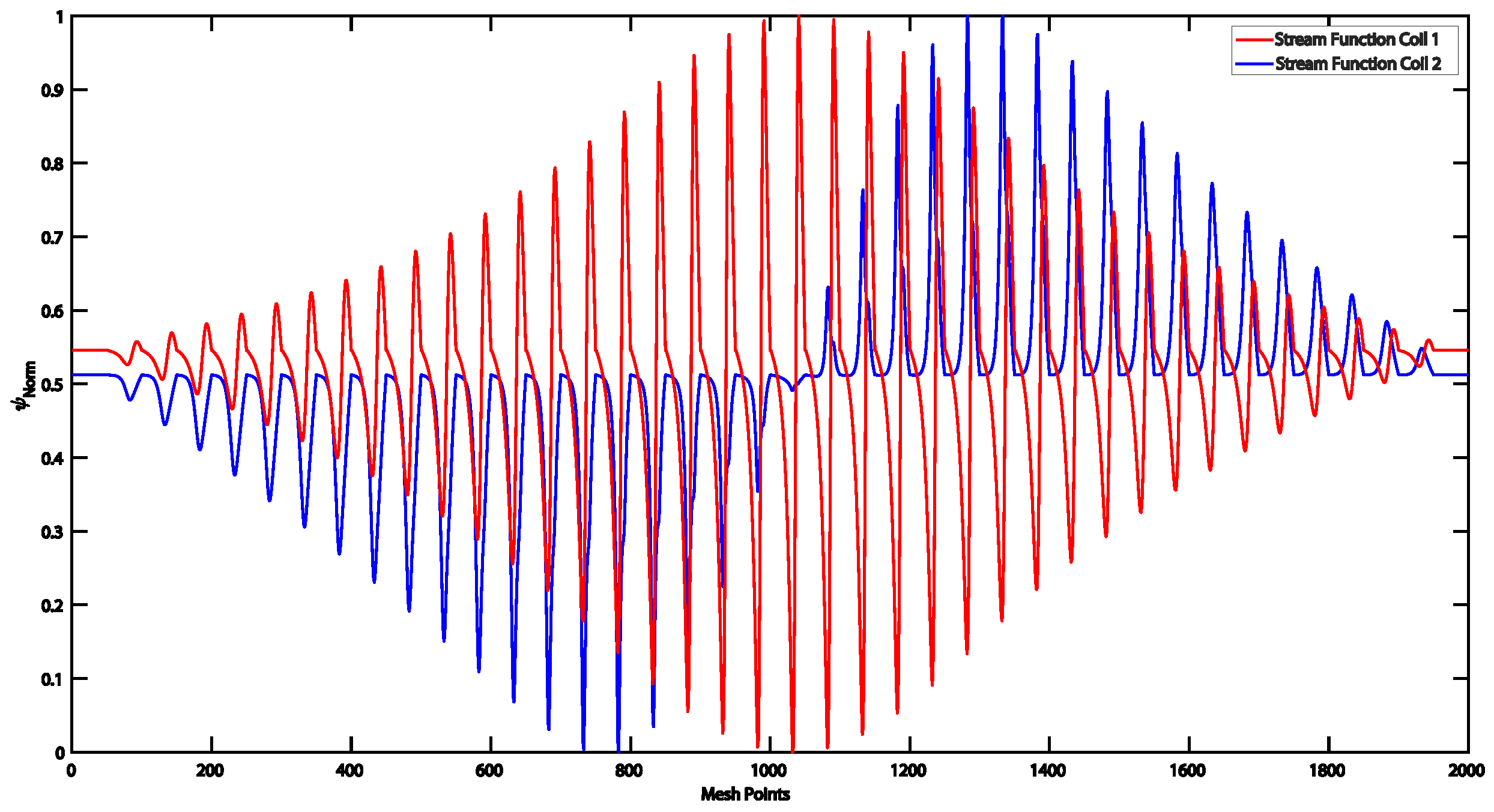
Appendix A.2. Design of Maximal Bx and By Coil for Magnetic Measurement Systems in a Space Missions

In the following, for the purpose of illustrating an application of the obtained theoretical results in this manuscript, we present the design of a planar coil over a (34 × 17 mm) PCBfor magnetic measurement systems in space missions. This coil was constructed with the aim of maximizing the magnetic field in a small and near region where a magnetic sensor capable of measuring the X and Y components of the B field is located. At the same time, resistance was minimized in order to avoid power dissipation.
Hence, the initial requirement that the coil had to satisfy was that it had to produce a maximal magnetic field in a region of interest (ROI) that was located in the same position as that of the sensor ( x = 22 mm , y = 6.5 mm , z = 1.25 mm ) , with its same dimensions (5.8 × 3.5 mm), formed by 200 points. Figure A1 illustrates the available surface for the coil design along with the ROI.
Figure A1. Representation of planar coil surface and region of interest (ROI) where optimal stream function φ is calculated.
Symmetry 13 00661 g0a1
In order to obtain stream function φ , which simultaneously maximizes B x and B y while minimizing power dissipation at the ROI, previously presented MOPs (16) and (17) were applied. Consequently, the current coil-design problem can be expressed as the following MOPs:
max B x C 1 φ 2 , min φ 2 , φ R n , max B y C 1 φ 2 , min φ 2 , φ R n , max B z C 1 φ 2 , min φ 2 , φ R n .
max α B x C 1 φ 2 2 + β B y C 1 φ 2 2 + γ B z C 1 φ 2 2 , min φ 2 , φ R n .
where B i R m × n stands for the matrix of the magnetic field in the i-th direction ( i = x , y , z ); R R n × n is the resistance matrix; n is the number of mesh points ( n = 2000 ); m is the number of ROI points ( m = 200 ); and α , β , and γ are constants that provide specific weights for maximizing each component of the field ( B x , B y , B z ). Due to the fact that it is only necessary to maximize the B x and B y components in the current case, weights were chosen such that α = β < γ (in concrete α = β = 1 and γ = 10 2 ).
Figure A2 shows the stream function solution from the (A1) and (A2) MOPs (red and blue functions, respectively) computed by using the theoretical model developed in [4,18,19]. Three different optimal stream functions were obtained from (A1) MOP ( φ x , φ y , φ z ). Consequently, the final φ 1 solution was calculated as linear combination φ 1 = α φ x + β φ y + γ φ z . However, stream function φ 2 is the final solution obtained from the (A2) MOP. As expected from the conclusions of the manuscript, the stream functions were not equal.
Figure A2. Stream functions obtained from Problems (A1) (Coil 1) and (A2) (Coil 2).
Symmetry 13 00661 g0a2
Furthermore, stream function contours over the coil surface can be considered to be the current wire path [30,31]. Accordingly, coil wires were designed as the stream function contour, as is depicted in Figure A3 and Figure A4, where the designed coils are different depending on the MOP.
Figure A3. Obtained wire paths from Problem (A1) over PCBsurface.
Symmetry 13 00661 g0a3
Figure A4. Obtained wire paths from Problem (A2) over the PCB surface.
Symmetry 13 00661 g0a4
In conclusion, as expected from the proposed theoretical model in this manuscript, the solutions of (A1) and (A2) were different; consequently, we could not conclude any relation between the two MOPs.

References

  1. Bishop, E.; Phelps, R.R. A proof that every Banach space is subreflexive. Bull. Am. Math. Soc. 1961, 67, 97–98. [Google Scholar] [CrossRef] [Green Version]
  2. Bishop, E.; Phelps, R.R. The support functionals of a convex set. In Sympos. Pure Mathematics; American Mathematical Society: Providence, RI, USA, 1963; Volume VII, pp. 27–35. [Google Scholar]
  3. Aizpuru, A.; García-Pacheco, F.J. A short note about exposed points in real Banach spaces. Acta Math. Sci. Ser. B (Engl. Ed.) 2008, 28, 797–800. [Google Scholar] [CrossRef]
  4. Cobos-Sánchez, C.; García-Pacheco, F.J.; Moreno-Pulido, S.; Sáez-Martínez, S. Supporting vectors of continuous linear operators. Ann. Funct. Anal. 2017, 8, 520–530. [Google Scholar] [CrossRef]
  5. García-Pacheco, F.J.; Naranjo-Guerra, E. Supporting vectors of continuous linear projections. Int. J. Funct. Anal. Oper. Theory Appl. 2017, 9, 85–95. [Google Scholar] [CrossRef]
  6. James, R.C. Characterizations of reflexivity. Stud. Math. 1964, 23, 205–216. [Google Scholar] [CrossRef] [Green Version]
  7. Lindenstrauss, J. On operators which attain their norm. Isr. J. Math. 1963, 1, 139–148. [Google Scholar] [CrossRef]
  8. García-Pacheco, F.J.; Rambla-Barreno, F.; Seoane-Sepúlveda, J.B. Q-linear functions, functions with dense graph, and everywhere surjectivity. Math. Scand. 2008, 102, 156–160. [Google Scholar] [CrossRef] [Green Version]
  9. García-Pacheco, F.J.; Puglisi, D. Lineability of functionals and operators. Stud. Math. 2010, 201, 37–47. [Google Scholar] [CrossRef]
  10. García-Pacheco, F.J. Lineability of the set of supporting vectors. Rev. R. Acad. Cienc. Exactas Fís. Nat. Ser. A Mat. RACSAM 2021, 115, 41. [Google Scholar] [CrossRef]
  11. Mititelu, C. Optimality and duality for invex multi-time control problems with mixed constraints. J. Adv. Math. Stud. 2009, 2, 25–34. [Google Scholar]
  12. Mititelu, C.; Treanţă, S. Efficiency conditions in vector control problems governed by multiple integrals. J. Appl. Math. Comput. 2018, 57, 647–665. [Google Scholar] [CrossRef]
  13. Treanţă, S.; Mititelu, C. Duality with (ρ,b)-quasiinvexity for multidimensional vector fractional control problems. J. Inf. Optim. Sci. 2019, 40, 1429–1445. [Google Scholar] [CrossRef]
  14. Treanţă, S.; Mititelu, C. Efficiency for variational control problems on Riemann manifolds with geodesic quasiinvex curvilinear integral functionals. Rev. R. Acad. Cienc. Exactas Fís. Nat. Ser. A Mat. RACSAM 2020, 114. [Google Scholar] [CrossRef]
  15. Choi, J.W.; Kim, M.K. Multi-Objective Optimization of Voltage-Stability Based on Congestion Management for Integrating Wind Power into the Electricity Market. Appl. Sci. 2017, 7, 573. [Google Scholar] [CrossRef] [Green Version]
  16. Susowake, Y.; Masrur, H.; Yabiku, T.; Senjyu, T.; Motin Howlader, A.; Abdel-Akher, M.; Hemeida, A.M. A Multi-Objective Optimization Approach towards a Proposed Smart Apartment with Demand-Response in Japan. Energies 2019, 13, 127. [Google Scholar] [CrossRef] [Green Version]
  17. Zavala, G.R.; García-Nieto, J.; Nebro, A.J. Qom—A New Hydrologic Prediction Model Enhanced with Multi-Objective Optimization. Appl. Sci. 2019, 10, 251. [Google Scholar] [CrossRef] [Green Version]
  18. Cobos Sánchez, C.; Garcia-Pacheco, F.J.; Guerrero Rodriguez, J.M.; Hill, J.R. An inverse boundary element method computational framework for designing optimal TMS coils. Eng. Anal. Bound. Elem. 2018, 88, 156–169. [Google Scholar] [CrossRef]
  19. Garcia-Pacheco, F.J.; Cobos-Sanchez, C.; Moreno-Pulido, S.; Sanchez-Alzola, A. Exact solutions to max‖x‖=1i=1Ti(x)‖2 with applications to Physics, Bioengineering and Statistics. Commun. Nonlinear Sci. Numer. Simul. 2020, 82, 105054. [Google Scholar] [CrossRef]
  20. Moreno-Pulido, S.; Garcia-Pacheco, F.J.; Cobos-Sanchez, C.; Sanchez-Alzola, A. Exact Solutions to the Maxmin Problem max‖Ax‖ Subject to ‖Bx‖ ≤ 1. Mathematics 2020, 8, 85. [Google Scholar] [CrossRef] [Green Version]
  21. Wassermann, E.; Epstein, C.; Ziemann, U.; Walsh, V. Oxford Handbook of Transcranial Stimulation (Oxford Handbooks), 1st ed.; Oxford University Press: New York, NY, USA, 2008. [Google Scholar]
  22. Romei, V.; Murray, M.M.; Merabet, L.B.; Thut, G. Occipital Transcranial Magnetic Stimulation Has Opposing Effects on Visual and Auditory Stimulus Detection: Implications for Multisensory Interactions. J. Neurosci. 2007, 27, 11465–11472. [Google Scholar] [CrossRef]
  23. Sánchez, C.C.; Rodriguez, J.M.G.; Olozábal, Á.Q.; Blanco-Navarro, D. Novel TMS coils designed using an inverse boundary element method. Phys. Med. Biol. 2016, 62, 73–90. [Google Scholar] [CrossRef]
  24. Marin, L.; Power, H.; Bowtell, R.W.; Cobos Sanchez, C.; Becker, A.A.; Glover, P.; Jones, I.A. Numerical solution of an inverse problem in magnetic resonance imaging using a regularized higher-order boundary element method. In Boundary Elements and Other Mesh Reduction Methods XXIX, WIT Trans. Model. Simul.; WIT Press: Southampton, UK, 2007; Volume 44, pp. 323–332. [Google Scholar] [CrossRef] [Green Version]
  25. Marin, L.; Power, H.; Bowtell, R.W.; Cobos Sanchez, C.; Becker, A.A.; Glover, P.; Jones, A. Boundary element method for an inverse problem in magnetic resonance imaging gradient coils. CMES Comput. Model. Eng. Sci. 2008, 23, 149–173. [Google Scholar]
  26. Mateos, I.; Ramos-Castro, J.; Lobo, A. Low-frequency noise characterization of a magnetic field monitoring system using an anisotropic magnetoresistance. Sens. Actuators A Phys. 2015, 235, 57–63. [Google Scholar] [CrossRef] [Green Version]
  27. Mateos, I.; Patton, B.; Zhivun, E.; Budker, D.; Wurm, D.; Ramos-Castro, J. Noise characterization of an atomic magnetometer at sub-millihertz frequencies. Sens. Actuators A Phys. 2015, 224, 147–155. [Google Scholar] [CrossRef] [Green Version]
  28. Mateos, I.; Sánchez-Mínguez, R.; Ramos-Castro, J. Design of a CubeSat payload to test a magnetic measurement system for space-borne gravitational wave detectors. Sens. Actuators A Phys. 2018, 273, 311–316. [Google Scholar] [CrossRef] [Green Version]
  29. Mateos, I.; Díaz-Aguiló, M.; Ramos-Castro, J.; García-Berro, E.; Lobo, A. Interpolation of the magnetic field at the test masses in eLISA. Class. Quantum Gravity 2015, 32, 165003. [Google Scholar] [CrossRef] [Green Version]
  30. Peeren, G. Stream function approach for determining optimal surface currents. J. Comput. Phys. 2003, 191, 305–321. [Google Scholar] [CrossRef] [Green Version]
  31. Brideson, M.; Forbes, L.; Crozier, S. Determining complicated winding patterns for Shim coils using stream functions and the target-field method. Concepts Magn. Reson. 2002, 14, 9–18. [Google Scholar] [CrossRef]
Publisher’s Note: MDPI stays neutral with regard to jurisdictional claims in published maps and institutional affiliations.

