The Additive Input-Doubling Method Based on the SVR with Nonlinear Kernels: Small Data Approach

Abstract

The problem of effective intellectual analysis in the case of handling short datasets is topical in various application areas. Such problems arise in medicine, economics, materials science, science, etc. This paper deals with a new additive input-doubling method designed by the authors for processing short and very short datasets. The main steps of the method should include the procedure of data augmentation within the existing dataset both in rows and columns (without training), the use of nonlinear SVR to implement the training procedure, and the formation of the result based on the author’s procedure. The authors show that the developed data augmentation procedure corresponds to the principles of axial symmetry. The training and application procedures of the method developed are described in detail, and two algorithmic implementations are presented. The optimal parameters of the method operation were selected experimentally. The efficiency of its work during the processing of short datasets for solving the prediction task was established experimentally by comparison with other methods of this class. The highest prediction accuracy based on both proposed algorithmic implementations of a method among all of the investigated ones was defined. The main areas of application of the developed method are described, and its shortcomings and prospects of further research are given.

1. Introduction

The effectiveness of prediction or classification using artificial intelligence tools depends heavily on the quality and quantity of training data [1]. A large amount of noisy data reduces the classification or prediction accuracy [2]. On the other hand, a short set of data makes it impossible to use machine learning to solve such tasks. Similar situations arise in economics during the promotion of a new product on the market, in materials science during the long and very expensive collection of observations of a specific object of study, in medicine during the collection of data from patients with rare diseases, and in many other areas [3]. If there are a sufficient number of observations for the implementation of training procedures and validation of the corresponding machine learning model, there are several advantages to using artificial intelligence to solve a specific applied task. In some cases, it saves material and time resources; in others, it provides the ability to establish an accurate diagnosis by an inexperienced doctor; and in others, it provides the ability to simulate a specific phenomenon or event without great expense. However, in most cases, it is not possible to collect more data samples of a specific short dataset [4]. If we talk about the need to process a limited set of data by artificial intelligence tools, there is a problem of finding and selecting the optimal method or algorithm. This is where problems of prediction accuracy, training speed, model overfitting, inability to validate the model, etc., arise due to lack of data [5].

If we talk about the application of simple data mining methods, they do not always provide the required efficiency. This significantly depends on the dataset, its volume, the number of attributes, the interconnections between them, etc. In cases of complex, nonlinear interconnections between a large numbers of short dataset input attributes, the use of simple linear models will not provide the necessary prediction accuracy [6]. That is why the use of simple models is limited to a very narrow class of tasks when processing short datasets. The situation can be corrected with the use of artificial intelligence tools: machine learning algorithms or artificial neural networks. Prediction by existing artificial intelligence tools in such cases can provide a significant increase in predicted accuracy. However, their use is accompanied by the need for a sufficient number of samples for training. In most such cases, the implementation of the training procedure is not possible due to the limited dataset. In cases where it is physically possible to perform, short datasets for training do not make this procedure effective at the appropriate level. This imposes several restrictions on the use of existing tools to solve several practical tasks in various fields. This situation is typical for both numerical data and other input information (e.g., images [7]).

A small data approach is topical area of research today for several reasons, presented, analyzed in detail and proven in [8]. However, a small number of practical tools based on artificial intelligence to effectively solve the problem have been developed to date.

Therefore, the aim of this paper is to design a new method for the effective processing of short datasets, which will provide high prediction accuracy with the minimum possible resources required for the implementation of the training procedure.

The main contribution of this paper can be summarized as follows:

• the design of an SVR-based additive input-doubling method, which provides increase of the prediction accuracy of regression modeling in case of processing short and very short sets of medical data; procedures for its training and application are developed;
• two algorithmic implementations of the developed method are investigated based on the use of two different nonlinear SVR kernels (rbf and polynomial);
• the optimal parameters of the developed algorithms are experimentally determined; the highest prediction accuracy of the proposed algorithms is established compared to other machine learning methods of this class.

The remainder of this paper is organized as follows: Section 2 contains the review and analysis of related works; mathematical descriptions of the classical SVR methods are described in Section 3. Section 4 contains basic provision of the axial symmetry of the response surface that forms the basis of the proposed method, as well as the mathematical formulations of the designed method. The results of the experimental modeling of two proposed algorithmic implementations of the designed method are shown in Section 5. Comparison results and discussion are presented in Section 6. The last section contains the conclusions and prospects for further research.

2. Related Works

A review of existing methods indicates two main areas of research in this field [9]:

-

ensemble learning;

-

numerical data augmentation.

The first of them is ensemble learning. The idea of the methods in this class is to use several models that are different from each other (either with respect to the type of algorithm or to one of the parameters of the same algorithm) to predict or classify based on the available dataset. As a result, the most accurate result is chosen from those obtained by voting or averaging. This approach is justified in areas where obtaining a large dataset is either very hard or impossible. In [4], the authors worked with just such a task. The study of single machine learning models did not provide sufficient accuracy, but the ensemble approach showed significantly better results. This is because each member of the ensemble is characterized by low bias but high variance, and the results of their work are averaged.

Another approach in this direction is study reported in [10]. The method of “multiple runs” developed by the authors consists of carrying out a large number of neural network runs with fixing of weight coefficients at each run and the selection of the most accurate result from among those obtained. It can also be interpreted as a kind of ensemble learning with a huge number of members. Each of them is characterized by unique (randomly selected) initial parameters, which provides a significant difference between them. The results in this case are not averaged, and the best value is chosen from among those obtained. The advantage of this approach is the ability to obtain a highly accurate result when processing short datasets. Fixing the weights of an artificial neural network provides the possibility to repeat the results of the experiment, thus opening up several possibilities for the practical application of the method. The disadvantage of methods of this class is the large amount of computing and energy resources required to implement such approaches. This is due to the need for parallel processing of the dataset by a large number of ensemble members (for example, [6]), or a large number of runs of the neural network to obtain the best value. In particular, in [10], 10,000 runs of an artificial neural network were performed to select the most accurate result.

The second large class of methods are methods of artificial expansion of the available short dataset (data augmentation methods). This approach involves artificially increasing the training dataset in order to increase the generalization properties of the machine learning algorithms or artificial neural networks that will be trained on it. This can increase the accuracy when solving specific application tasks. The authors in [11] divide these methods into two major subclasses: columnar methods and row-wise methods. Each of them has several groups that combine common features.

If we talk about a simple method of artificial expansion of the training set of numerical data [12], then it is necessary to know the laws of distribution in the middle of the set, which is not a trivial task in the case of a limited set of data. That is why such methods do not always show a significant increase in the accuracy of regressors or classifiers, but significantly increase the resources required for the operation of the latter [13]. If we talk about the use of artificial neural networks to generate new observations based on a set of existing ones, this approach has paid off in the image processing field [14]. Recognition or classification tasks based on deep learning are only effective if there is a large learning set. Otherwise, it makes no sense to use, for example, Deep Convolutional Neural Networks. In recent years, Generative Adversarial Networks (GAN) have been used quite frequently with this aim. They are able to generate a large number of artificial images, thus increasing the accuracy of neural network classifiers. However, if we talk about numerical data, then there are not many developments in this direction. One of the most recent studies is that reported in [15]. The authors developed a method of combining GAN and vector Markov Random Field. The latter tool generates synthetic data according to the concept of the method, and GAN analyzes the similarity of that data with the real data. The GAN stops working when it cannot distinguish the synthesized vector from the real data. The proposed approach showed higher performance compared to existing approaches on synthetic and real data. The authors of [16] developed a new numerical data generator based on the training of GAN. Experimental studies confirmed the effectiveness of this method, which increases the accuracy of machine learning algorithms, but not in all cases. Simulation of this method was performed on large datasets. This condition provided the opportunity for effective GAN training to generate new data, and, accordingly, good results. However, in the case of very small datasets, this method did not show an improvement, due to the insufficient number of samples for training.

In [17,18], the authors developed a new method of processing short and very short datasets that combines the advantages of the two classes of methods described above. The idea of the approach is to artificially expand the training dataset using a very simple procedure proposed by the authors, which provides an increase in the generalization properties of nonlinear classifiers or regressors. This is typical of the data augmentation methods class. The application procedure involves the implementation of the author’s prediction procedure based on vectors, which contains the attributes of the input vector and all vectors of the initial training dataset. Here, we are talking about averaging the predicted results based on the extended vectors fed to the input. This procedure is typical of the ensemble approach. In [17,18], the authors demonstrated an increase in the accuracy of SVR prediction based on a very short set of medical data.

In [19], an improved version of the developed method was presented. First, the authors used the RBF neural network as a basic nonlinear artificial intelligence tool to implement the training procedure. Actually, the algorithm for artificial expansion of the training set remained the same as in [17,18]; however, the application procedure was changed. Where [17,18] had formed only one temporary dataset, the results of which were averaged using a special procedure, the advanced method involved the formation of two such datasets, using the attributes of the input vector with unknown output, and all vectors of the initial training dataset. The difference between the two temporary samples is the order of combining the above vectors and the formation of the resulting variable. The authors demonstrated a significant increase in the prediction accuracy compared with [17,18] compared to the basic regressor. However, this method requires the selection of a large number of additional parameters in the model, and it is quite time-consuming and resource-intensive.

3. Support Vector Machine

The method for effectively processing short datasets developed in this paper is based on the use of the classical machine learning algorithm, Support Vector Machine (SVM) [20], in the case of solving the classification task, or Support Vector Regression (SVR) [21], in the case of solving the regression task. The principles of SVM and SVR are the same. That is why this section provides an explanation of the classical SVM. SVR is the basis for the proposed algorithmic implementations of the proposed method. Its only difference is the use of nonlinear kernels: rbf or polynomial kernels.

Therefore, let’s consider the basic mathematical foundation of the classic SVM.

The prominent scientists V. N. Vapnik and A. Ya Chervonenkis developed the classical SVM in 1963. The main features of its implementation were presented in several works, in particular in [20,21]. Let’s consider the basics of this machine learning method.

Let observations for training D be given, consisting of n objects with p parameters [22]:

$$\mathrm{D}={\left\{\left(x_i,y_i\right)|x_i\in R^p,y_i\in \left\{-1,1\right\}\right\}}_{i=1^n},$$

(1)

where y is binary class for $x_i$.

Each point $x_i$ is a vector of p dimensionality.

It is required to find the hyperplane of maximum difference that separates the observations $y_i=1$ and observations$y_i=-1$.

Any hyperplane is defined as a set of points x satisfying the condition: w * x − b = 0, where * is the scalar product of the normal to the hyperplane by the vector x.

Parameter $\frac{b}{\parallel w\parallel }$ defines the displacement of the hyperplane relative to the origin along the normal w.

Two hyperplanes can be chosen if the training data is linearly separable. They must separate the data without intersection and the distance between them must be maximized.

The area bounded by two hyperplanes is called the “difference (margin)”. These hyperplanes are given by the equations:

$$\begin{array}{l}w*x-b=1,\\ w*x-b=-1.\end{array}$$

(2)

Using geometric interpretation, the distance between these hyperplanes is defined as $\frac{2}{\parallel w\parallel }$.

In order for the distance to be maximum, we minimize $\parallel w\parallel$.

To exclude all points from the strip, we must make sure for all observations that it is true:

$$w*x_i-b\ge 1,$$

(3)

for $x_i$ from the first class,

$$w*x_i-b\le -1,$$

(4)

$x_i$ from the second class.

Respectively:

$$y_i\left(w*x_i-b\right)\ge 1,$$

(5)

for $0\le i\le n$.

Next, we solve the optimization problem analytically: $\parallel w\parallel \to min$.

The optimization problem presented above is difficult to solve, since it depends on the norm w in square root. Then, $\frac{1}{2}{\parallel w\parallel }^2$is used without changing the solution (at least the original and modified equations have the same w and b).

The quadratic optimization problem is formed as a result of the previous transformations.

More precisely, we need to find the minimum:

$$\frac{1}{2}{\parallel w\parallel }^2\to min,$$

(6)

with restrictions:

$$y_i\left(w*x_i-b\right)\ge 1,$$

(7)

for $0\le i\le n$.

By introducing Lagrange multipliers, a constrained problem can be expressed as an unconstrained problem:

$$\underset{w,b}{\min } \underset{a\ge 0}{\max }\left\{\frac{1}{2}{\parallel w\parallel }^2-{\displaystyle \sum }_{i=1}^n{a}_i*\left[y_i\left(w*x_i-b\right)-1\right]\right\}.$$

(8)

Describing the classification rules in their unconditional form shows that the maximum margin of the hyperplane and, therefore, the classification problem is only a function of support vectors.

Observations for learning are on the edge. If $\parallel w\parallel =w\ast w$ and $={\displaystyle \sum }_{i=1}^n{a}_i{y}_i{x}_i$, it can be shown that the second form of support vector machine solves the optimization problem:

Maximization for $a_i$ is given as:

$$L\left(a\right)={\displaystyle \sum }_{i=1}^n{a}_i-\frac{1}{2}{\displaystyle \sum }_{i,j}^n{a}_i{a}_j{y}_i{y}_j{x}_i^T{x}_i={\displaystyle \sum }_{i=1}^n{a}_i-\frac{1}{2}{\displaystyle \sum }_{i,j}^n{a}_i{a}_j{y}_i{y}_{j}k\left(x_i,x_i\right), a_i\ge 0.$$

(9)

Limitation from minimization for b: ${\displaystyle \sum }_{i=1}^n{a}_i{y}_i=0$. The kernel is defined as: $k\left(x_i,x_i\right)=x_i{x}_j$. W can be calculated due to the conditions:

$$w={\displaystyle \sum }_{i,j}^n{a}_{i}a{y}_i{x}_i.$$

(10)

Support vector machine belongs to the family of general linear classifiers, but it can solve different nonlinear tasks using different kernels. In our case, this is very important, because the designed method will provide good results using only nonlinear kernels ([19]).

A special feature is that SVM can simulate the minimum empirical classification error and maximize the geometric difference (margin).

Let’s consider the designed method based on the SVR with nonlinear kernels.

4. Proposed Method

4.1. Machine Learning in the Case of Short Datasets Using Axial Symmetry of the Response Surface

In [8,10,23], the problems of modeling the nonlinear response surfaces of multidimensional functions that are represented by short data samples using machine learning is described in detail. Existing data augmentation methods for solving this task are characterized by several shortcomings, described in the first section of the paper. The authors of this study designed a method for creating extended data samples based on the principles of forming a dataset that corresponds to the principles of axial symmetry. The essence of this procedure is to mirror the half of the formed response surface relative to the axial plane (straight) itself. This procedure consists of the specular reflection of half of the response surface in a plane (line).

To better understand the developed procedure, we will demonstrate the results of its visual representation by example of a one-dimensional task of function reproduction $y=x^2$, where $x=0\to 1$ with step equal 0.1. It should be noted that this example was chosen for simplicity, and the method itself retains its versatility regardless of the dimension of the task. We believe that the number of specified interpolation points (in this example 11) is insufficient to permit the use of known procedures for training, testing and validation by machine learning methods, such as SVR. Let’s perform the following operations: $y_1={x_1}^2,y_2={x_2}^2,z=y_1-y_2$ for $x_1,x_2=0\to 1$ with step 0.1.

Let’s plot (Figure 1) the function of two variables $z=F(x_1,x_2)$ where $y_1={x_1}^2,y_2={x_2}^2,$ for all possible pairs of combined vectors $x_1,x_2=0\to 1$ with step 0.1, the output of which is formed as $z=y_1-y_2$.

As can be seen from Figure 1, the response surface, which is represented by 121 interpolation points, is mirror symmetric with respect to the line $x_1=x_2$, and we consider 121 vectors $x_1,x_2,z$ sufficient for the implementation of machine learning procedures.

Let us present the formulation and solution of the task for an arbitrary dimension of the data space, where the principle of axial symmetry is always preserved.

4.2. SVR-Based Additive Input-Doubling Method

The classic version of SVR, in particular in the implementation of [24], is quite fast, provides an unambiguous solution, and demonstrates several practical applications when processing small datasets [25,26]. However, when it comes to very short datasets, which is typical for medicine, its accuracy is not satisfactory. The developed method is based on the introduction of new variables:

$$z_{k,i}=(y_k-y_i);z_{i,k}=(y_i-y_k),$$

(11)

where $y_i$ is the output signal for the i-th vector of the training sample, $i=\overline{1,N}$; and $y_k$ is the output signal for the current k-th vector.

After performing simple identical transformations, and taking the sums from both parts of Equation (11), we obtain:

$${\displaystyle \sum _{i=1}^N{z}_{k,i}}=N{y}_k-{\displaystyle \sum _{i=1}^N{y}_i},$$

(12)

$${\displaystyle \sum _{i=1}^N{z}_{i,k}}={\displaystyle \sum _{i=1}^N{y}_i}-N{y}_k.$$

(13)

Subtracting Equation (13) from Equation (12), we obtain:

$$y_k=\frac{{\displaystyle \sum _{i=1}^N{Z}_{k,i}-{\displaystyle \sum _{i=1}^N{Z}_{i,k}}}}{2N}+\frac{{\displaystyle \sum _{i=1}^N{y}_i}}{N}.$$

(14)

The obtained expression (14) is the basis of the developed SVR-based additive input-doubling method. This method provides an opportunity to increase the accuracy of the nonlinear machine learning method (only nonlinear [19]) with satisfactory results in terms of the speed of its work (because it is about processing short datasets). In addition, data augmentation, as one of the steps in the developed method, increases its generalization properties.

Like the classic SVR [24], and existing methods [17,18] the developed method works in two modes: learning and application.

4.2.1. Training Mode

The first step of the iterative training mode is the formation of a new, artificially expanded dataset (by both rows and columns). It will contain N² pairs of vectors ${\overline{x}}_i{\overline{x}}_j\to z_{i,j}^{augm},i=1,N;j=1,N;t=1,N^2$ (extensions by columns) that will be formed by combining all available vectors of the training dataset, where N is the number of existing observations (extensions by rows).

The output signal for each new vector will be formed as follows: $z_{i,j}=(y_i-y_j)$.

The second step is to implement the SVR training procedure with a pre-selected kernel of the method based on the thus-formed training dataset. It should be noted that the first algorithmic implementation of the method requires the use of an rbf kernel. The second algorithmic implementation uses a polynomial kernel. In both cases, it is necessary to choose the optimal values of the required parameters.

4.2.2. Application Mode

The peculiarity of this mode is that the output signal for a particular k observation is unknown. It must be predicted. The main stages of the procedure of application of the developed method, in contrast to [17,18], include the implementation of such steps.

In the first step of the procedure, it is necessary to form a set of N extended vectors, each of which will contain a set of features of both the input k vector and each of the N vectors of the initial training dataset: ${\overline{x}}_k{\overline{x}}_i$, where $i=1,N$. In addition, in contrast to [17,18], another set of N extended vectors is formed in this step. In this case, in the first place will be each of the N vectors of the initial dataset, and in the second, the current vector, the output signal of which must be predicted: ${\overline{x}}_i{\overline{x}}_k$, where $i=1,N$. As a result, we obtain two temporary datasets.

The aim of forming two additional datasets in this step is the possibility of compensating for errors of different signs in the final procedure of forming the output signal of the developed method [19].

The next step of the procedure involves the use of a pre-trained SVR with a corresponding core to predict the output signals $z_{i,k}^{pred},z_{k,i}^{pred}$ for each temporary vector of both generated datasets in the previous step: ${\overline{x}}_i{\overline{x}}_k\to z_{i,k}^{pred},{\overline{x}}_k{\overline{x}}_i\to z_{k,i}^{pred}$, where $i=1,N$.

The last step of the application procedure is to substitute the obtained values of $z_{i,k}^{pred},z_{k,i}^{pred}$ into expression (15) to form the searched-for value of the output signal $y^{pred}$ for the k-th input vector:

$$y^{pred}=\frac{{\displaystyle \sum _{i=1}^N{z}_{k,i}^{pred}-{\displaystyle \sum _{i=1}^N{z}_{i,k}^{pred}}}}{2N}+\frac{{\displaystyle \sum _{i=1}^N{y}_i}}{N}.$$

(15)

It should be noted that the first term of the right-hand side of Equation (11) provides:

• the mutual compensation of errors of various signs;
• the principles of ensemble learning by averaging the result.

This provides a significant increase in the prediction accuracy of the SVR when processing small-sized and middle-sized datasets.

5. Modeling and Results

Modeling of the SVR-based additive input-doubling method was performed on a computer with the following parameters: DELL, Intel Core i7-10510U (1.8–4.9), 8 Gb RAM. Performance evaluation was conducted based on Mean Absolute Error (MAE), Root Mean Square Error (RMSE) and training time [27,28].

The task of the prediction of calcium concentration (millimoles per liter) in the analysis of human urine was solved in the paper. This analysis is important for assessing calcium metabolism when examining a patient with breast cancer, myeloma, hypoalbuminemia, hypomagnesaemia, chronic renal failure, and in monitoring the treatment of vitamin D deficiency (rickets) in pediatrics [29]. The semi-quantitative method for determining this parameter [29] requires the presence of several reagents and is quite time consuming [30].

Experimental studies were performed on a short medical dataset [31]. It contains 79 vectors, each of which is characterized by six independent attributes (indicator of the presence of calcium oxalate crystals; the urea concentration; the specific gravity of the urine; the osmolality of the urine; the conductivity of the urine; the pH reading of the urine).

Table 1. Short dataset.

Variable’s Title	MIN Value	MEAN Value	MAX Value
The pH reading of the urine	4.76	6.042	7.94
The osmolarity of the urine	187.00	613.61	1236.00
Indicator of the presence of calcium oxalate crystals	0.00	0.436	1.00
The urea concentration in millimoles per liter	10.00	264.141	620.00
The conductivity of the urine	5.10	20.901	38.00
The specific gravity of the urine	1.01	1.018	1.04
The calcium concentration in millimoles per liter	0.17	4.161	14.34

summarizes the basic characteristics of the dataset. A detailed analysis of the dataset is given in [31].

After preprocessing procedures, two vectors were removed from the set as they contained gaps. As a result, modeling was performed on 77 vectors, 80% of which were randomly selected for training and 20% for testing procedures.

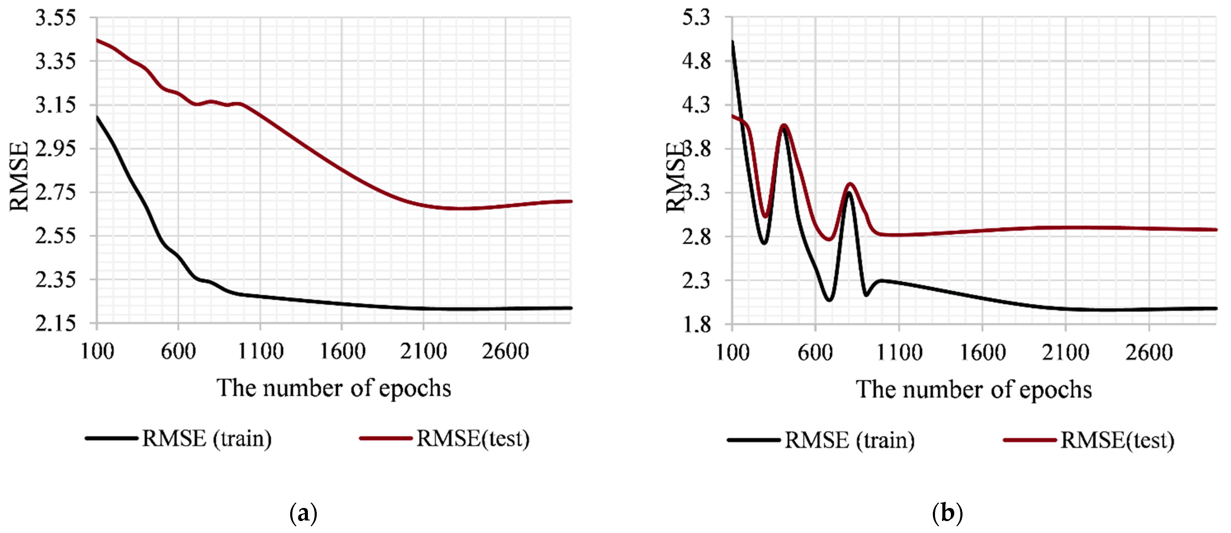
To easily reproduce the results of the developed method by other researchers, the authors chose a known and available implementation of SVR [24] with two nonlinear kernels (rbf and polynomial). Since SVR, which is the basis of the developed method, involves the implementation of an iterative training procedure, this paper investigated the influence of the number of epochs on the results of the method. The experiment was performed by changing the number of epochs from 100 to 3000 for both algorithmic implementations of the developed SVR-based additive input-doubling method. The results of this study are shown in Figure 2.

As can be seen from Figure 2, increasing the number of epochs of the training procedure reduces the errors of both algorithmic implementations of the method in both the training and the application modes. It should be noted that the additive input-doubling method based on SVR with the rbf kernel shows a more stable result compared to the algorithmic implementation based on the polynomial kernel (the interval of 100–800 epochs was taken into account). The stage of error saturation of the first algorithm begins from 2000 epochs, while the second begins from 1000 epochs. This statement is true for both MAE and RMSE (Figure 1). Further increase in the number of epochs of algorithms does not increase the accuracy of their work, but increases the duration of the training procedure. Accordingly, these values are selected as optimal for the operation of each of the proposed algorithmic implementations of the developed method during the processing of the investigated dataset.

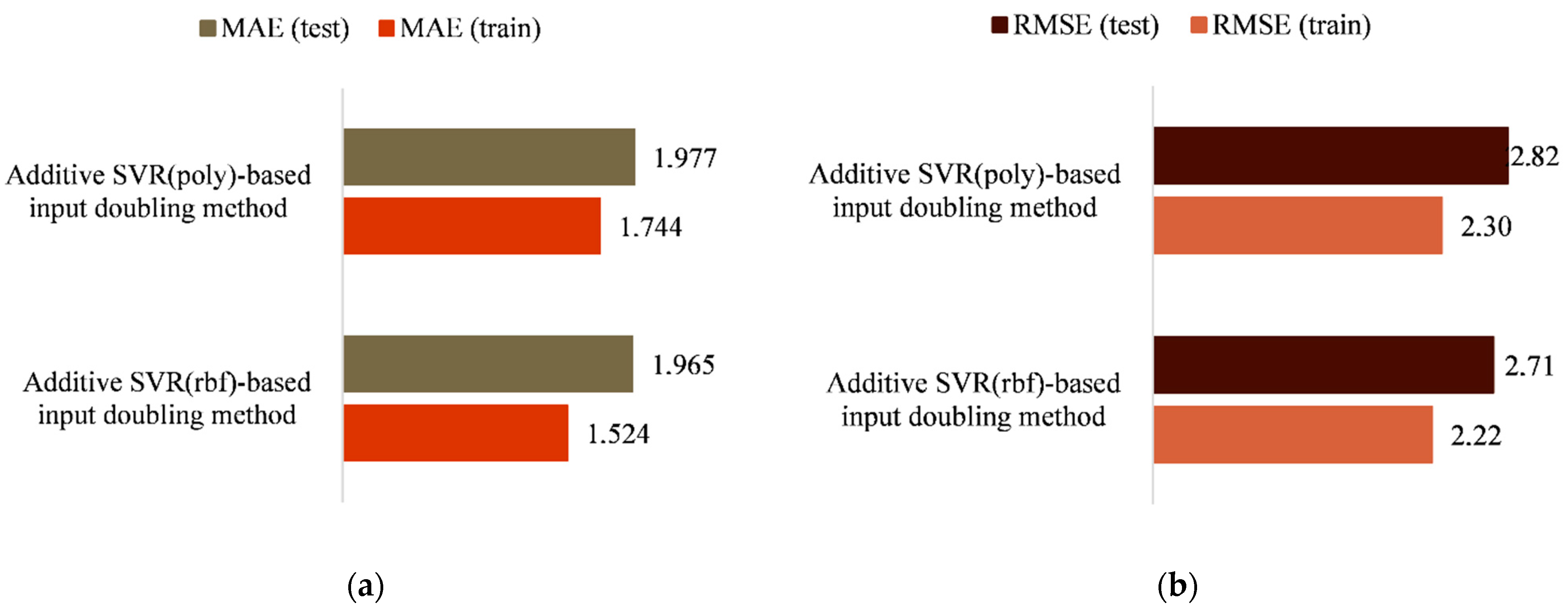
The software implementation of SVR from [24], which is taken as a basis in this study, does not provide for the possibility of changing the number of rbf centers when training the first proposed algorithm. Therefore, this option is selected by default. The advantage of this situation is the ability for other researchers to easily reproduce the results of the proposed algorithm [32,33]. With regard to the second algorithmic implementation of the developed method, the high values of the degree of the polynomial cause a significant increase in the duration of the training procedure, in particular by increasing the dimension of the input data space. In addition, experimental studies have shown that such an increase does not provide the expected increase in prediction accuracy. In particular, for the third-degree polynomial (the default parameter), with other things being equal, the errors in the application mode were MAE = 1.97, RMSE = 2.82. When choosing the second-degree polynomial, the errors were MAE = 2.65, RMSE = 3.46, and when this parameter was equal to 4, MAE = 2.24, RMSE = 2.93. That is why the third-degree polynomial was chosen as the optimal value of the second algorithmic implementation of the proposed method. A visualization of the results obtained for both algorithms using RMSE and MAE can be seen in Figure 3.

By choosing the optimal parameters for both algorithms, the time required for their training can be determined. Specifically, the duration of the training procedure for the first and second algorithmic implementation of the method was 0.624 and 0.178 s, respectively.

In this work, we also tested the developed method on another short set of medical data. This is available in [10]. The task was to predict the compressive strength of the trabecular bone. The dataset consists of only 35 vectors. The results of the modeling for the two algorithmic implementations of the designed method, as well as a comparison with existing methods, are given in Appendix A, Figure A1.

6. Comparison and Discussion

A comparison of the efficiency of both algorithmic implementations of the additive input-doubling method was carried out with several existing methods in this class. Specifically, these were:

• SVR(rbf)-based input-doubling method [17];
• SVR(poly)-based input-doubling method [18];
• Support Vector Regression with rbf kernel [24];
• Support Vector Regression with polynomial kernel [24];
• Adaptive Boosting [24];
• Stochastic Gradient Descent [24].

The comparison was based on MAE, RMSE and training time. The operating parameters of the existing methods were the same as those developed. It should be noted that methods 3 and 4 used the initial dataset to implement the training procedure (61 vector). Methods 1 and 2 used an extended dataset according to the procedures described for the developed method.

The results of experimental modeling of all investigated methods for both the training and application modes are summarized in

Table 2. Performance indicators for all methods investigated.

Method	MAE	RMSE	Training Time, Seconds
Additive SVR(rbf)-based input-doubling method	Training mode
	1.524	2.219	0.624
	Test mode
	1.965	2.707	-
Additive SVR(poly)-based input-doubling method	Training mode
	1.744	2.296	0.178
	Test mode
	1.977	2.823	-
SVR(rbf)-based input-doubling method	Training mode
	1.524	2.219	0.624
	Test mode
	2.315	3.057	-
SVR(poly)-based input-doubling method	Training mode
	1.775	2.413	0.178
	Test mode
	2.187	3.093	-
SVR(poly)	Training mode
	2.065	2.815	0.001
	Test mode
	2.937	3.728	-
SVR(rbf)	Training mode
	2.029	2.810	0.002
	Test mode
	2.662	3.449	-
Adaptive Boosting *	Training mode
	0.449	0.603	0.239
	Test mode
	2.317	3.06	-
Stochastic Gradient Descent **	Training mode
	2.883	4.075	0.002
	Test mode
	2.578	4.115	-

* the results obtained for the next parameters of the AdaBoost algorithm: DecisionTreeRegressor (max_depth = 4), n_estimators = 300 of the scikit-learn library when the others parameters were equal; ** the results obtained for the next parameters of the SGD algorithm: loss = ‘huber’, alpha = 0.0001 of the scikit-learn library when the others parameters were equal.

. For better illustration, the results are also presented in Figure 4.

As can be seen from Table 2 and Figure 4, the least accurate results for the studied dataset were obtained by the SGD and AdaBoost algorithms. In both cases, there is an overfitting, which is a typical issue when processing short datasets. SGD demonstrates the highest training speed, but the least accurate results.

Similar results were obtained using the classical SVR. The experimental results showed the largest errors when using both kernels (rbf and polynomial) of this classical machine learning algorithm in comparison with all other methods.

Significantly better results were obtained for the algorithms of the existing input-doubling method [17,18]. In particular, when using the polynomial kernel of the existing method [18], the difference between the errors of MAE and RMSE compared to the corresponding implementation of the classical SVR were 0.75 and 0.635, respectively. For algorithms based on rbf kernel, these differences were MAE = 0.347, RMSE = 0.392. If we compare the increase in accuracy when applying the developed method in comparison with [17,18], then the corresponding error differences are: MAE = 0.35, RMSE = 0.35 for the rbf kernel and MAE = 0.21, RMSE = 0.27 for the polynomial kernel. In summary, both algorithmic implementations of the developed method show a significant increase in accuracy compared to the classical SVR [24]. In particular, the use of the rbf kernel shows differencess in the errors of both methods MAE = 0.697, RMSE = 0.742, and the use of the polynomial kernel shows MAE = 0.96, RMSE = 0.905. At first glance, this may seem like a small result, but when it comes to small and very small datasets, it is a good result.

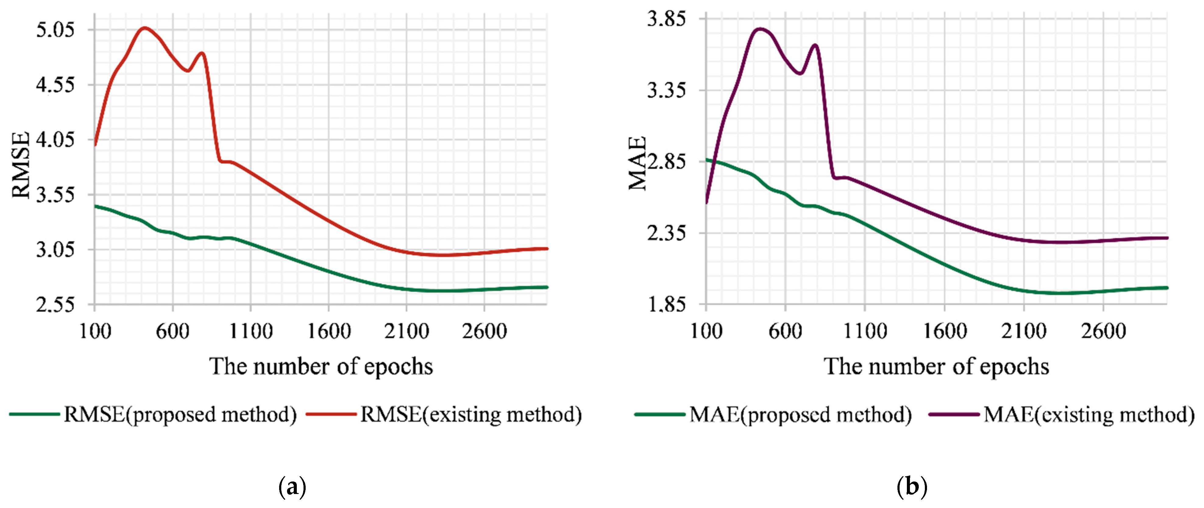
Since the developed method and the algorithms [17,18] of the existing method are very similar, let us consider the results in more detail. Training took place on the same extended dataset, and the only significant difference was the different procedures of the application mode and the forming of the output signal. Figure 2 shows the dynamics of changes in the accuracy of the four algorithmic implementations of the studied methods (the two developed algorithms and the two existing algorithms [17,18]) when changing the number of epochs of the training algorithm under otherwise-equal conditions.

Let us consider the case of using the rbf kernel as a basis for the developed and existing methods (Figure 5a,b). As can be seen from Figure 5, the existing algorithm shows a significantly higher error value with a number of epochs <800. Then, the decreasing stage begins (800–2000 epochs), which, starting from 2000 epochs, goes into the stage of saturation. The latter is characterized by the fact that the increase in the number of epochs and therefore the increasing duration of the training procedure does not increase the prediction accuracy. If we consider the errors of the application mode for the proposed algorithm, then, first, both errors of the proposed algorithm are significantly lower than those for the existing one throughout the investigated interval. Secondly, in the interval of 100–800 epochs, there are no such significant “jumps” of errors in comparison with the existing method. This is due to the possibility of compensating for errors of different signs, which is provided by the procedure (15) of generating the output signal of the developed method. The stage of saturation of the error, as for the existing method, begins at 2000 epochs. However, within the interval of 2000–3000 epochs, the method shows a lower error that is within the value of 0.3 for RMSE and 0.35 for MAE.

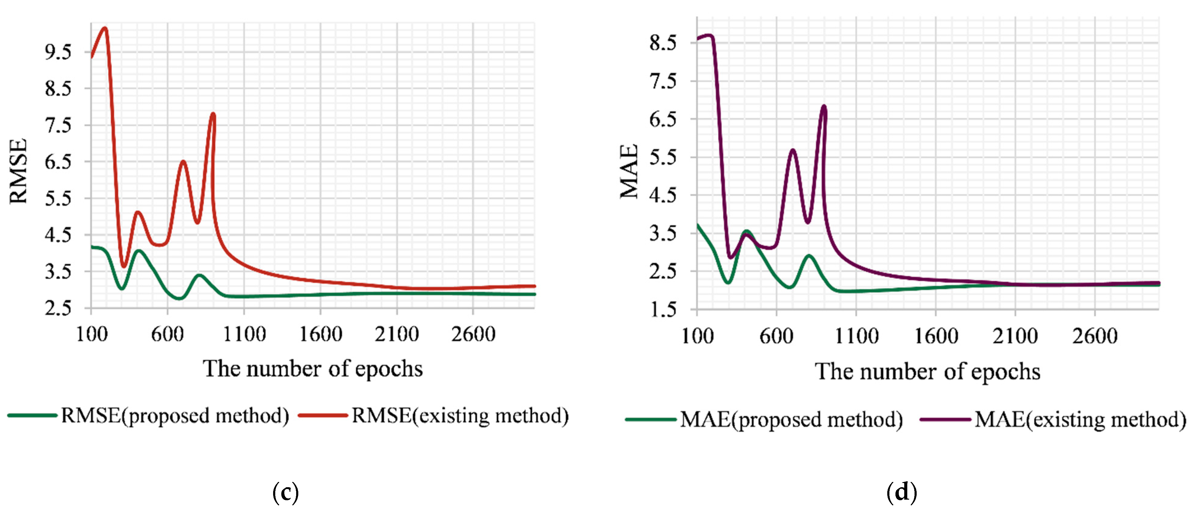
The algorithmic implementation of the developed and existing [18] methods based on the polynomial kernel showed slightly different results (Figure 5c,d). In the interval of 300–800 epochs, the existing method showed sharp fluctuations in both errors, and here the general trend of error growth (MAE and RMSE) can be observed. In the case of the developed algorithm, these fluctuations were not so sharp, and the general trend was a decrease in error. At the saturation stage (2000–3000 epochs), both algorithms showed very close prediction accuracy, although the developed algorithm demonstrated slightly smaller error values.

The initial training dataset for modeling contained 61 vectors. It was used when applied to the classic SVR with the polynomial and rbf kernels [24]. According to data augmentation procedures, which were the same for the developed Additive SVR-based input-doubling method and for the existing SVR-based input-doubling method [17,18], training took place on an extended set of 3712 data vectors. It is obvious that such an increase of data will significantly affect the duration of the training procedure. In addition, the features of each vector were doubled, according to the two methods. This increase in the dimension of the input data space also affected the duration of the training procedure. If we talk about the duration of training of algorithmic implementations of both the developed methods and the existing ones [17,18], then for both corresponding algorithms it will be the same. However, at the same time, higher indicators of the prediction accuracy of both of the proposed algorithms in comparison with the existing were obtained.

If we compare the duration of the training procedure of the developed method and the classical SVR, there is a significant increase for the proposed method. However, this is because the training set in this case has grown by 61 times and is characterized by double the dimensions of the input data space. In addition, because the method is designed to process short datasets, provides a significant increase in prediction accuracy, and the time of its training does not exceed 1 s, this shortcoming can be ignored. The proposed approach can be used in different application areas, as in [34,35,36,37].

7. Conclusions

Effective small data mining is an important issue today. This paper presents a new approach to solving this task. The authors developed an additive input-doubling method to improve prediction accuracy based on a limited dataset. SVR with nonlinear kernels is the basis of its work. Algorithmic implementation of the method involves the use of a data augmentation procedure in rows and columns to form a new training dataset, the use of SVR to implement the training procedure on such a set, calculating the required value according to the developed procedure (15). A feature of this method, in contrast to the existing ones, is a new application procedure that involves the creation of two temporary datasets from the current vector and all available vectors of the training dataset. In addition, the paper develops and mathematically substantiates a new procedure for generating the output signal, which differs significantly from the existing ones [17,18]. The introduction of additional elements in (15) provides the possibility of correcting errors of different signs of this equality, and as a consequence, increases the prediction accuracy.

Experimental modeling was performed using a short set of medical data. The initial training sample contained only 61 vectors. The authors described the procedures for selecting the parameters of the method, experimentally determining its optimal values. The comparison was made using SVR-based methods of this class. The developed method in both of its algorithmic implementations demonstrated a significant increase in prediction accuracy compared to the classical SVR with two nonlinear kernels, which was the aim of this study. In particular, the increase in accuracy for the algorithm based on the rbf kernel was MAE = 0.697, RMSE = 0.742, and for the algorithm with the polynomial kernel, MAE = 0.96, RMSE = 0.905.

The method described in the paper and its results are also important from a theoretical point of view. First, it opens up a new direction in the development of effective methods for processing short datasets using existing machine learning tools. Secondly, it is possible to construct different algorithmic implementations of the proposed method using nonlinear artificial neural networks. Third, further development and modification of the method will provide high-precision processing of datasets of different volumes. Fourth, the practical value of such developments will be reflected in various areas of human activity, from economics to materials science.

The main limitation of this study is the evaluation of the results of the method on only two datasets. However, the designed method demonstrated the highest prediction accuracy on both short datasets. The disadvantage of the designed method is a significant increase in the duration of the training procedure compared to the parent regressor due to a significant increase in the training dataset in terms of both columns and rows. To avoid this, we plan to conduct further research in the following directions:

• the development of input-doubling methods and additive input-doubling methods based on the use of a high-speed RBF-SGTM neural-like structure and its modifications [38]. This will reduce the duration of the training procedure of the developed methods;
• the development of a weighted input-doubling method and additive input-doubling method by replacing expression (15) with a neural network, in particular a non-iterative, corrective SGTM neural-like structure. This will allow the implementation of the procedure for weighing the results (15) instead of the usual summation, which will increase the prediction accuracy;
• the application of clustering and input doubling methods for efficient processing of middle-sized datasets;
• the evaluation of the designed method for the solution of other real tasks in different application areas using a large number of short datasets.