
Control Charts for Joint Monitoring of the Lognormal Mean and Standard Deviation


Department of Statistics, Feng Chia University, Taichung 40724, Taiwan
Symmetry 2021, 13(4), 549; https://doi.org/10.3390/sym13040549
Submission received: 27 January 2021
/
Revised: 9 March 2021
/
Accepted: 23 March 2021
/
Published: 26 March 2021
(This article belongs to the Special Issue New Advances and Applications in Statistical Quality Control)
Abstract
:The Shewhart - and S-charts are most commonly used for monitoring the process mean and variability based on the assumption of normality. However, many process distributions may follow a positively skewed distribution, such as the lognormal distribution. In this study, we discuss the construction of three combined - and S-charts for jointly monitoring the lognormal mean and the standard deviation. The simulation results show that the combined lognormal - and S-charts are more effective when the lognormal distribution is more skewed. A real example is used to demonstrate how the combined lognormal - and S-charts can be applied in practice.
1. Introduction
Control charts are widely used in statistical process control (SPC) for monitoring and detecting out-of-control processes. The research on constructing control charts for monitoring normal processes has been extensively studied. Most control charts are designed to monitor either the process mean or the process variability, but it is usually desirable to simultaneously monitor the process mean and the process variability because both may change at the same time. A change in the standard deviation usually leads to out-of-control signals on the mean chart. When the distribution of quality characteristics is normal, the Shewhart -chart [1] is one of the most commonly used control charting techniques for monitoring the process mean, while the Shewhart S-chart is commonly used to monitor the process variability. However, in many manufacturing applications, the quality variable typically follows a positively skewed distribution, such as the lognormal distribution. For example, the percent viscosity increase (PVI) of an engine oil after it has been put to an accelerated aging test for a specific period of time is a critical quality dimension of engine oil in the automotive industry. Engineering experience indicates that the PVI follows a lognormal distribution. In this case, it is very important to simultaneously monitor the mean and the standard deviation of the PVI based on a lognormal distribution.
In general, the implementation of a control chart is done in two stages, also known as Phase I control and Phase II monitoring. In Phase I control, in order to evaluate the variation of the process over time, assess the process stability, and estimate the in-control process parameters, one collects and analyzes certain amounts of historical data. In Phase II monitoring, one collects data sequentially and monitors the process in real time to quickly detect changes in the process parameters.
In the literature, there have been several studies on constructing control charts for monitoring the lognormal mean or the lognormal standard deviation. In monitoring the lognormal mean, a modified control chart using the sample ratio was proposed by Morrison [2]. A control chart for monitoring the “geometric midrange” of a lognormal distribution was developed by Ferrell [3]. A control chart for sequentially testing the arithmetic mean of a lognormal distribution was constructed by Joffe and Sichel [4]. A simple heuristic method for constructing the - and R- charts using the weighted variance (WV) method with no assumption on the form of the distribution was proposed by Bai and Choi [5]. Castagliola [6] proposed a new control chart devoted to the monitoring of skewed populations. Huang et al. [7] discussed the control charts for the lognormal mean based on the confidence intervals of the lognormal mean. In monitoring the standard deviation, Abu-Shawiesh [8] presented a simple approach for robustly estimating the process standard deviation based on the median absolute deviation. Adekeye and Azubuike [9] derived the limits for control charts using the median absolute deviation for monitoring non-normal processes. Adekeye [10] proposed modified control limits based on the median absolute deviation. Huang et al. [11] proposed a control chart for monitoring the standard deviation of a lognormal process based on an approximate confidence interval of the lognormal standard deviation. Karagöz [12] proposed an asymmetric control limit for a range chart under a non-normal distributed process. Liao and Pearm [13] presented a modified weighted standard deviation index for the capability of a lognormal process. Shaheen et al. [14] presented a monitoring control chart based on lognormal process variation using a repetitive sampling scheme. Omar et al. [15] proposed an efficient approach for monitoring a positively skewed process. The control charts for jointly monitoring the mean and the standard deviation of a lognormal distribution are not as well established as those for a normal distribution. McCracken and Chakraborti [16] gave an overview of control charts for joint monitoring of the mean and variance. Yang [17] proposed a single-average loss control chart to monitor a process’s mean and variability. Chen and Lu [18] proposed a new sum-of-squares exponentially weighted moving average (SSEWMA) chart using auxiliary information—called the AIB-SSEWMA chart—for jointly monitoring the process mean and variability .
In this study, we discuss three combined - and S-charts for jointly monitoring the mean and the standard deviation of a lognormal process: (1) The first combined charts are the conventional combined Shewhart - and S-charts. (2) The second combined charts are constructed based on the median absolute deviation method. (3) The third combined charts are the combined lognormal - and S-charts based on the methodologies studied in Huang et al. [7] and Huang et al. [11], respectively. The performances of these combined control charts are evaluated and compared in terms of the average run length (ARL), where the run length is defined as the number of samples taken before the first out-of-control signal alerts on a control chart [19].
The rest of this paper is organized as follows. The aforementioned combined - and S-charts for jointly monitoring the lognormal mean and standard deviation are discussed in Section 2. Section 3 is devoted to assessing the performance of the combined - and S-charts. A real example from the automotive industry is given in Section 4 to demonstrate how the aforementioned combined - and S-charts can be used in practice. Concluding remarks are given in Section 5.
2. The Methodologies
In this section, we discuss three combined - and S-charts for jointly monitoring the lognormal mean and the standard deviation. Let , , , be m samples, each with size n, following the lognormal distribution with parameters and , with a probability density function
and, consequently, , which follow a normal distribution with the mean, , and variance, . Let and denote the mean and the standard deviation of the lognormal distribution such that and .
2.1. The Combined Shewhart - and S-Charts
The Shewhart - and S-charts are based on the assumption that the distribution of the quality characteristic is normal. The upper control limit (UCL) and lower control limit (LCL) of the combined Shewhart - and S-charts are given by
and
respectively, where and are multipliers chosen to satisfy a specific in-control chart performance and [1,19].
If the parameters and are unknown, they can be estimated by and using data obtained from Phase I control data. Let and be the sample mean and sample standard deviation of the ith sample, , that is, and , respectively. The sample grand mean is , and the average of the m standard deviations is . Then, the parameters and are estimated by and , respectively. Therefore, the control limits of the combined Shewhart - and S-charts are estimated by
and
respectively, where and are multipliers that depend on n and the desired in-control average run length (ARL).
When Phase II joint monitoring begins, independent samples, each of size n, are repeatedly taken from the process. Assume that the true in-control parameter and are equal to and , respectively, for each sample, ; one calculates and and plots and against the sampling sequence, respectively. An out-of-control signal is detected when is below or above , or when is below or above .
2.2. The Combined Median Absolute Deviation - and S-Charts
The median absolute deviation (MAD), which measures the deviation of the data from the sample median, was first studied by Hampel [20]. It is a more robust scale estimator than the sample standard deviation and is often used as an initial value for computing more efficient and robust estimators. The MAD for a random sample, , is defined as follows:
where b is a constant used to make the estimator consistent for the parameter of interest and is the sample median of , . If the sample observations are normally distributed, the constant b is equal to 1.4826, and the statistic is an unbiased estimator of the standard deviation (Rousseeuw and Croux ) [21], where is a function of the sample size n; the values of were derived and tabulated in Abu-Shawiesh [8].
Based on the conventional Shewhart principle, when the parameters and are unknown, they can be estimated by and using data obtained from Phase I control data. Let be the average median absolute deviation, where MAD is the median absolute deviation of the ith sample, . The parameter and can be estimated by and , respectively. Hence, the control limits of the combined - and S-charts based on MAD are estimated by
and
respectively, where and are multipliers that depend on n and the desired ARL.
When Phase II joint monitoring begins, independent samples, each of size n, are repeatedly taken from the process. For each sample, , one calculates and and plots and against the sampling sequence, respectively. An out-of-control signal is detected when is below or above , or when is below or above .
2.3. The Combined Lognormal - and S-Charts
Based on the conventional Shewhart -chart, if the parameters and are unknown, they can be replaced by the estimators and obtained from Phase I in-control data. According to Huang et al. [7], let and be the sample mean and the sample standard deviation of the ith sample, , respectively. The grand sample mean of Y is , and the average of the m standard deviations is . The parameters and can be estimated by and , respectively. Therefore, the control limits of the lognormal -chart are estimated using
where is set to satisfy a desired ARL.
According to Huang, et al. [11], there are two cases for the standard deviation. For the first case of , the control limits of the lognormal S-chart are estimated using
where is a multiplier that depends on n and the desired ARL. For the second case of , the control limits of the lognormal S-chart are estimated using
When Phase II joint monitoring begins, independent samples, each of size n, are repeatedly taken from the process. For each sample, , in the case of , one calculates and plots and against the sampling sequence, where and . An out-of-control signal is detected if the plotting statistic is below or above , or when the plotting statistic falls below or above . For the case of , one computes and plots and against the sampling sequence. An out-of-control signal is detected if the plotting statistic is below or above , or when the plotting statistic falls below or above .
Remark 1.
The population standard deviation σ is usually unknown and needs to be estimated in practice. It can be estimated by utilizing data collected from Phase I control, when the process was in control. Based on the estimate, one can then decide whether to use Case I or Case II to construct the lognormal S-chart.
3. Chart Performance Evaluations and Comparisons
In this section, we conduct a simulation study to compare the performance of the combined lognormal - and S-charts with the combined MAD - and S-charts and the conventional Shewhart - and S-charts in terms of the ARL.
3.1. Simulated Settings
Since , we set such that the mean of the lognormal distribution remains unchanged. Let be the value of the in-control parameter. As discussed earlier, the control limits need to be determined using Phase I observations and will depend on , the subgroup size n, and the number of Phase I samples m. Therefore, we approximate the control limits of the three combined - and S-charts using simulations for various values of and combinations of and 100, as well as and 10. The value of is set to be between 0.2 and 2.0, with an increment of 0.2. The multipliers of the three combined control charts are calibrated to have an overall ARL that is approximately equal to 370. Note that the considered ARL for the three combined control charts is conditional on the estimated UCL and LCL. Here, we describe how the simulation is conducted for the combined lognormal - and S-charts, as it is similar for the other two combined charts. Given , m, and n, the following steps are carried out:
Step 1: Choose a value of and a value of , and generate m independent samples of n observations each from a lognormal distribution with a mean of 1 and a standard deviation of . Compute the and , and calculate the and using either Equation (1) if or Equation (2) if .
Step 2: Repeatedly generate samples of n observations each from a lognormal distribution with a mean of 1 and standard deviation of . For each sample, calculate the two plotting statistics for the -chart and S-chart, respectively. Then, evaluate whether the plotting statistic for the -chart exceeds or goes below ; next, evaluate whether the plotting statistic for the S-chart exceeds or goes below . Stop when it does, and denote the number of samples generated by RL.
Step 3: Repeat Step 2 times, resulting in RL, . Calculate the simulated in-control average run length .
Step 4: If , stop. If , return to Step 1. Choose a larger if and a smaller if .
The multipliers of the three combined - and S-charts are given in Table 1 and Table 2 for different values of . Note that the multipliers of these three combined - and S-charts increase when () increases.
Denote the out-of-control process parameters by and , where . Given , we simulated the ARL for the three combined charts in the same way as in Steps 2 and 3, which were mentioned earlier. The out-of-control ARLs (ARLs) of the three combined - and S-charts are summarized in Table 3 and Table 4 () and Table 5 and Table 6 ().
3.2. Discussion of Results
According to the assessment of the numerical results summarized in Table 3, Table 4, Table 5 and Table 6, the combined lognormal - and S-charts perform better than the other two combined - and S-charts when . Nevertheless, the ARLs of the combined lognormal - and S-charts are larger than those of the other two combined - and S-charts when . Note that smaller values of correspond to smaller values of , under which the lognormal distribution is more symmetric. Therefore, when is small, which means that the data are more symmetric, the combined lognormal - and S-charts are less effective than the combined Shewhart - and S-charts and the combined MAD - and S-charts. On the other hand, as becomes larger, the lognormal distribution becomes more skewed, thus making the combined lognormal - and S-charts more effective in detecting changes in and than the other two combined control charts.
4. Example from the Automotive Industry
In this section, we present a real example to illustrate the applicability of the combined lognormal - and S-charts. The ASTM D7320 Ref Oil Data were provided by the Test Monitoring Center [22]. In order to assess the engine oil quality, especially for new vehicles, the percent viscosity increase (PVI), which follows a lognormal distribution, needs to be tested. In this dataset, the quality of three reference oils—Ref Oils 434, 435, and 438—needs to be tested. We collected 50 samples, each of size 10, for each of these three reference oils, and used them to construct the Phase I control charts.
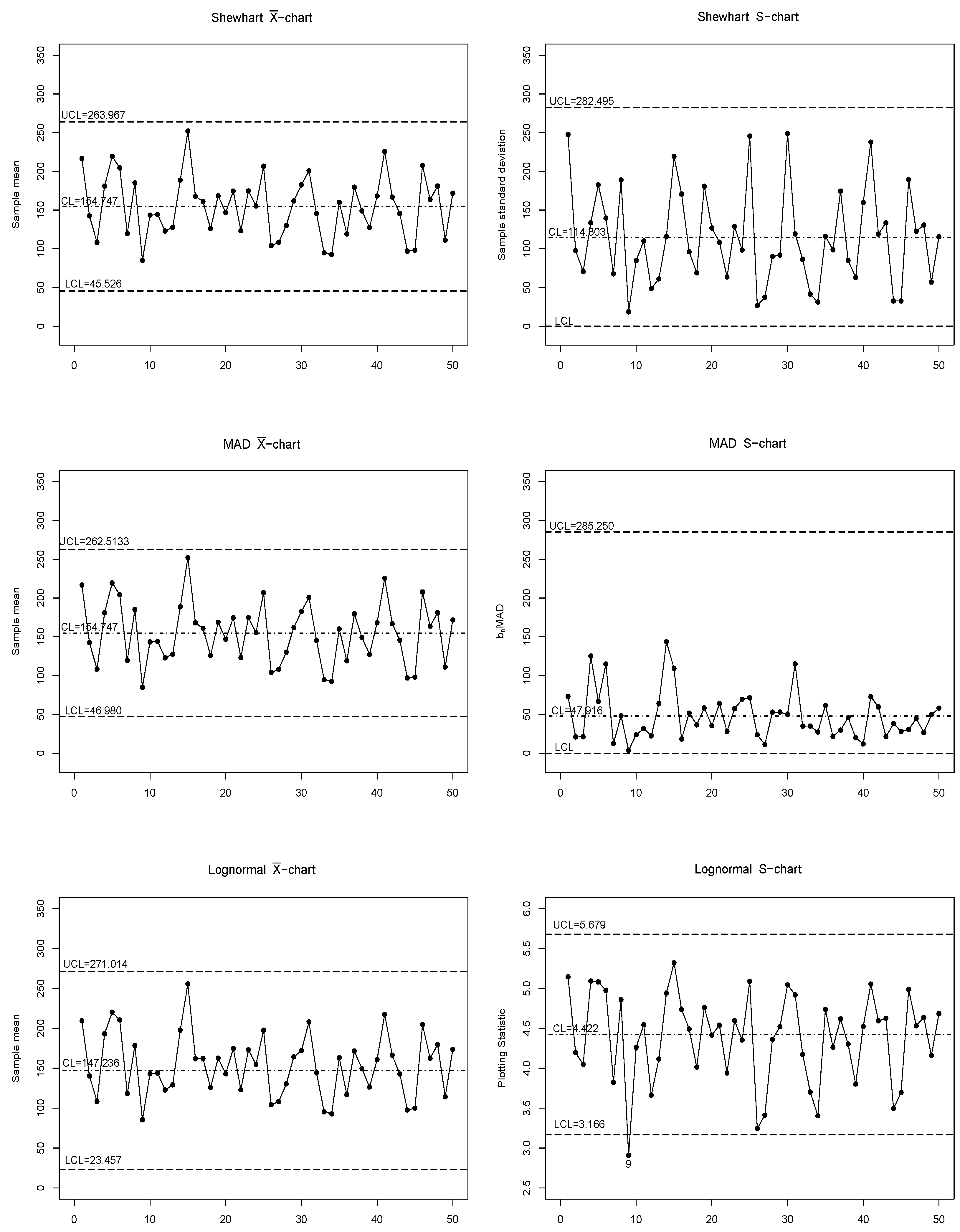
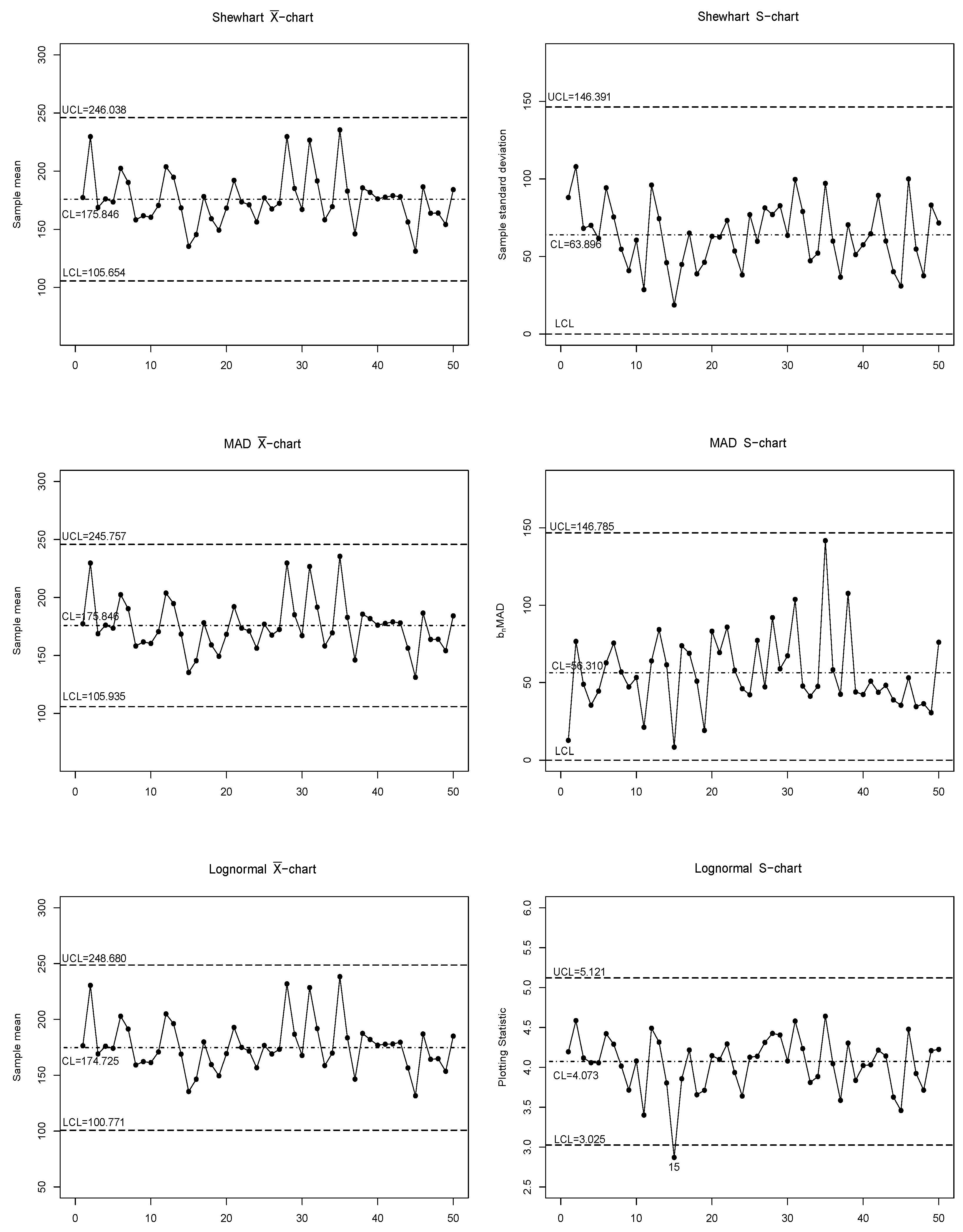
The multipliers of the three combined - and S-charts were calibrated to have a Type I error approximately equal to 0.0027 in order to have a fair comparison. Summarized in Table 7 are the upper and lower control limits of the three combined - and S-charts, the estimated means, and the estimated standard deviations of the PVI for the three reference oils. Figure A1, Figure A2 and Figure A3 show the three combined - and S-charts for Ref Oils 434, 435, and 438, respectively.
Neither the combined Shewhart - and S-charts nor the combined MAD - and S-charts showed any out-of-control samples for Ref Oil 434 (Figure A1). On the other hand, sample 9 was outside the control limits of the lognormal S-chart. Consequently, the control limits were recalculated without sample 9 for the Phase II joint monitoring of the combined lognormal - and S-charts for Ref Oil 434. Similarly, there were no out-of-control samples in the combined Shewhart - and S-charts or the combined MAD - and S-charts for Ref Oil 435 (Figure A2), while sample 15 was out of control on the lognormal S-chart. Hence, the control limits of the combined lognormal - and S-charts for Ref Oil 435 were recalculated without sample 15 for the Phase II joint monitoring. As for Ref Oil 438 (Figure A3), none of the three combined -charts and S-charts showed any out-of-control samples.
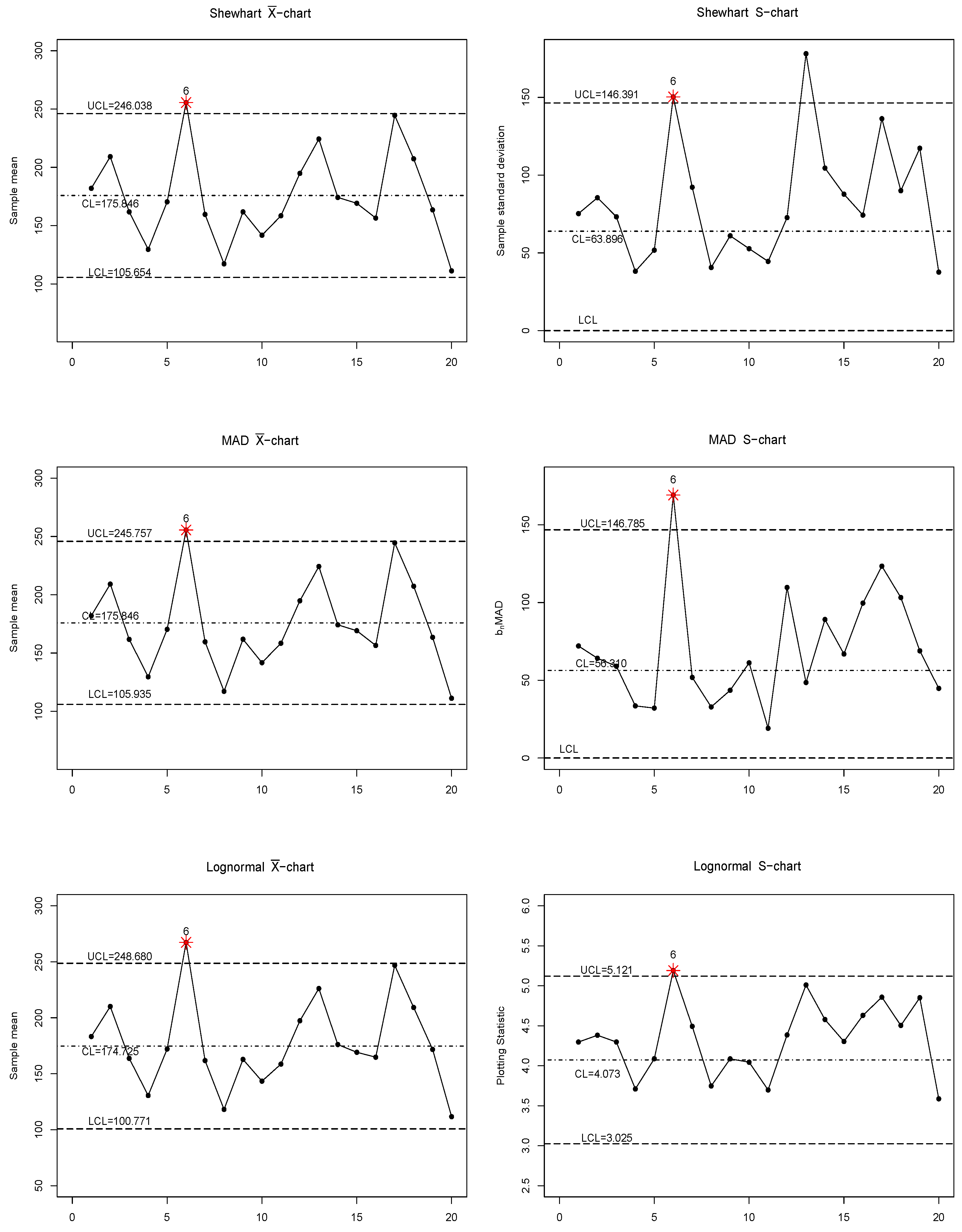
The sample mean and the sample standard deviation of the PVI calculated based on the Phase I samples were used as the “true mean" and the “true standard deviation", respectively, in the simulation process because the true population mean and population standard deviation were unknown. The mean and the standard deviation of the PVI were respectively assumed to be 154.747 and 127.376, 175.846 and 66.963, and 94.647 and 20.828 for Ref Oils 434, 435, and 438, respectively. For Phase II monitoring, 20 new samples with a subgroup size of 10 were generated when changed from to and changed from to . Note that the 20 new samples were computer simulated, not obtained from additional samples using the ASTM test method. All combined - and S-charts were tuned to produce an overall ARL that was approximately equal to 370. The resulting control charts for Ref Oils 434, 435, and 438 are shown in Figure A4, Figure A5 and Figure A6, respectively.
For Ref Oil 434 (Figure A4), the combined lognormal - and S-charts detected out-of-control signals at samples 5 and 4 in the - and S-charts, respectively, while the combined Shewhart - and S-charts triggered at samples 8 and 11 in the - and S-charts, respectively. In addition, out-of-control signals were detected at sample 8 in both the MAD - and S-charts. For Ref Oil 435 (Figure A5), out-of-control signals were detected on sample 6 in both the Shewhart - and S-charts and both the MAD - and S-charts. At the same time, out-of-control signals also appeared at sample 6 in both the lognormal - and S-charts. As for Ref Oil 438 (Figure A6), the combined Shewhart - and S-charts detected out-of-control signals at samples 6 and 2 in the - and S-charts, respectively, while the combined MAD - and S-charts detected at sample 6 in both charts. In addition, out-of-control signals were detected at sample 6 in both the lognormal - and S-charts.
5. Conclusions
In this study, we discuss the construction of three combined - and S-charts for jointly monitoring the mean and the standard deviation of the lognormal distribution. The simulation studies show that the combined lognormal - and S-charts have good performance when the underlying lognormal distribution is more skewed. The practical application of the combined lognormal - and S-charts is also demonstrated in a real example.
The numerical results of the current work indicate that for skewed non-normal processes, it is possible to construct more effective control charts for monitoring the process mean, process variability, or both based on the actual process distribution. This is at least the case for lognormal processes. It would be worth it to investigate how to construct more effective control charts for other skewed non-normal processes.
Remark 2.
As for other skewed non-normal processes, the process mean or process variability may need to be approximated first, and these can be estimated using Phase I in-control data. Based on the conventional Shewhart - and S-charts, one can construct the control limits of - and S-charts for monitoring the process mean or process variability under other skewed non-normal processes.
Funding
This research was funded by by Ministry of Science and Technology, MOST 108-2118-M-035-005-MY3, Taiwan.
Institutional Review Board Statement
Not applicable.
Informed Consent Statement
Not applicable.
Data Availability Statement
The data presented in this study are available on request from the corresponding author.
Acknowledgments
The author would like to thank the editor and the reviewers for their valuable suggestions and constructive comments. The author also wants to thank Arthur B. Yeh at Bowling Green State University for his help and insightful suggestions.
Conflicts of Interest
The author declares no conflict of interest.
Appendix A
For Phase I, the three combined - and S-charts are shown in Figure A1, Figure A2 and Figure A3 for Ref Oils 434, 435, and 438, respectively. For Phase II monitoring, the resulting control charts for Ref Oils 434, 435, and 438 are shown in Figure A4, Figure A5 and Figure A6, respectively.
Figure A1.
The three combined - and S-charts for the PVI of Ref Oil 434 in Phase I.

Figure A2.
The three combined - and S-charts for the PVI of Ref Oil 435 in Phase I.

Figure A3.
The three combined - and S-charts for the PVI of Ref Oil 438 in Phase I.

Figure A4.
The three combined - and S-charts for the PVI of Ref Oil 434 in Phase II.

Figure A5.
The three combined - and S-charts for the PVI of Ref Oil 435 in Phase II.

Figure A6.
The three combined - and S-charts for the PVI of Ref Oil 438 in Phase II.

References
- Shewhart, W.A. Economic quality control of manufactured product. Bell Syst. Tech. J. 1930, 9, 364–389. [Google Scholar] [CrossRef]
- Morrison, J. The lognormal distribution in quality control. Appl. Stat. 1958, 7, 160–172. [Google Scholar] [CrossRef]
- Ferrell, E.D. Control charts for lognormal universe. Ind. Qual. Control 1958, 15, 4–6. [Google Scholar]
- Joffe, A.D.; Sichel, H.S. A chart for sequentially testing observed arithmetic means from lognormal populations against a given standard. Technometrics 1968, 10, 605–612. [Google Scholar] [CrossRef]
- Bai, D.S.; Choi, I.S. X¯ and R control charts for skewed populations. J. Qual. Technol. 1995, 27, 120–131. [Google Scholar] [CrossRef]
- Castagliola, P. X¯ control chart for skewed populations using a scale weighted variance method. Int. J. Reliab. Qual. Saf. Eng. 2000, 7, 237–252. [Google Scholar] [CrossRef]
- Huang, W.H.; Wang, H.; Yeh, A.B. Control charts for the log-normal mean. Qual. Reliab. Eng. Int. 2016, 32, 1407–1416. [Google Scholar] [CrossRef]
- Abu-Shawiesh, M.O.A. A simple robust control chart based on MAD. J. Math. Stat. 2008, 4, 102–107. [Google Scholar]
- Adekeye, K.S. Modified simple robust control chart based on median absolute deviation. Int. J. Stat. Probab. 2012, 1, 91–95. [Google Scholar] [CrossRef] [Green Version]
- Adekeye, K.S.; Azubuike, P.I. Derivation of the limits for control charts using the median absolute deviation for monitoring non-normal process. J. Math. Stat. 2012, 8, 37–41. [Google Scholar]
- Huang, W.H.; Yeh, A.B.; Wang, H. A control chart for the log-normal standard deviation. Qual. Technol. Quant. Manag. 2018, 15, 1–36. [Google Scholar] [CrossRef]
- Karagöz, D. Asymmetric control limits for range chart with simple robust estimator under the non-normal distributed process. Math. Sci. 2018, 12, 249–262. [Google Scholar] [CrossRef] [Green Version]
- Liao, M.Y.; Pearn, W.L. Modified weighted standard deviation index for adequately interpreting a supplier’s lognormal process capability. Proc. Inst. Mech. Eng. Part B J. Eng. Manuf. 2019, 233, 999–1008. [Google Scholar] [CrossRef]
- Shaheen, U.; Azam, M.; Aslam, M. A control chart for monitoring the lognormal process variation using repetitive sampling. Qual. Reliab. Eng. Int. 2020, 36, 1028–1047. [Google Scholar] [CrossRef]
- Omar, M.H.; Arafat, S.Y.; Hossain, M.; Riaz, M. Inverse Maxwell Distribution and Statistical Process Control: An Efficient Approach for Monitoring Positively Skewed Process. Symmetry 2021, 13, 189. [Google Scholar] [CrossRef]
- McCracken, A.K.; Chakraborti, S. Control charts for joint monitoring of mean and variance: An overview. Qual. Technol. Quant. Manag. 2013, 10, 17–36. [Google Scholar] [CrossRef]
- Yang, S.F. Using a Single Average Loss Control Chart to Monitor Process Mean and Variability. Commun. Stat. Simul. Comput. 2013, 42, 1549–1562. [Google Scholar] [CrossRef]
- Chen, J.H.; Lu, S.L. A New Sum of Squares Exponentially Weighted Moving Average Control Chart Using Auxiliary Information. Symmetry 2020, 12, 1888. [Google Scholar] [CrossRef]
- Montgomery, D.C. Statistical Quality Control, 8th ed.; John Wiley & Sons (Asia) Pte. Ltd.: Hoboken, NJ, USA, 2019. [Google Scholar]
- Hampel, F.R. The influence curve and its role in robust estimation. J. Am. Stat. Assoc. 1974, 69, 383–393. [Google Scholar] [CrossRef]
- Rousseeuw, P.J.; Croux, C. Alternatives to the median absolute deviation. J. Am. Stat. Assoc. 1993, 88, 1273–1283. [Google Scholar] [CrossRef]
- D02 Committee. ASTM D7320 Test Method for Evaluation of Automotive Engine Oils in the Sequence IIIG, Spark-Ignition Engine; ASTM International: West Conshohocken, PA, USA, 2018. [Google Scholar]

Table 1.
The multipliers of the three combined - and S-charts based on different values of when the sample with the subgroup size and 10. (ARL).
Table 1.
The multipliers of the three combined - and S-charts based on different values of when the sample with the subgroup size and 10. (ARL).
| n | Shewhart | MAD | Lognormal | |||||
|---|---|---|---|---|---|---|---|---|
| -Chart | S-Chart | -Chart | S-Chart | -Chart | S-Chart | |||
| 5 | 0.2 | 0.20 | 3.18 | 3.92 | 3.62 | 4.89 | 3.42 | 4.31 |
| 0.4 | 0.41 | 3.64 | 6.56 | 4.47 | 7.55 | 4.14 | 3.92 | |
| 0.6 | 0.65 | 4.41 | 10.43 | 5.86 | 12.68 | 5.31 | 3.58 | |
| 0.7 | 0.79 | 4.97 | 11.53 | 5.93 | 16.97 | 6.22 | 3.54 | |
| 0.8 | 0.95 | 5.51 | 12.41 | 7.19 | 22.76 | 7.43 | 3.49 | |
| 0.9 | 1.12 | 6.27 | 14.67 | 10.49 | 26.48 | 8.85 | 3.51 | |
| 1.0 | 1.31 | 7.10 | 17.30 | 13.13 | 33.17 | 9.04 | 4.07 | |
| 1.2 | 1.79 | 9.37 | 23.99 | 20.59 | 56.47 | 10.45 | 3.88 | |
| 1.4 | 2.47 | 11.70 | 34.12 | 34.33 | 93.66 | 11.23 | 3.74 | |
| 1.6 | 3.45 | 14.53 | 44.21 | 54.21 | 150.35 | 13.06 | 3.63 | |
| 1.8 | 4.95 | 19.82 | 52.31 | 85.53 | 256.64 | 24.56 | 3.51 | |
| 2.0 | 7.32 | 21.98 | 64.76 | 148.05 | 427.10 | 30.88 | 3.41 | |
| 10 | 0.2 | 0.20 | 3.28 | 4.33 | 3.45 | 4.50 | 3.44 | 3.78 |
| 0.4 | 0.41 | 3.66 | 6.62 | 4.12 | 7.97 | 3.86 | 3.60 | |
| 0.6 | 0.65 | 4.14 | 10.90 | 5.38 | 14.11 | 4.48 | 3.39 | |
| 0.7 | 0.79 | 4.28 | 11.20 | 5.92 | 16.88 | 5.17 | 3.56 | |
| 0.8 | 0.95 | 5.77 | 14.24 | 7.84 | 25.05 | 5.27 | 3.38 | |
| 0.9 | 1.12 | 6.88 | 16.74 | 9.98 | 32.49 | 6.00 | 3.31 | |
| 1.0 | 1.31 | 7.70 | 19.66 | 12.06 | 44.17 | 6.12 | 4.13 | |
| 1.2 | 1.79 | 8.31 | 32.31 | 22.67 | 73.78 | 9.75 | 3.25 | |
| 1.4 | 2.47 | 10.49 | 38.49 | 34.00 | 95.11 | 10.86 | 3.26 | |
| 1.6 | 3.45 | 15.70 | 48.70 | 59.27 | 161.38 | 13.18 | 4.48 | |
| 1.8 | 4.95 | 20.48 | 64.48 | 97.42 | 277.53 | 23.99 | 3.09 | |
| 2.0 | 7.32 | 24.28 | 71.28 | 175.14 | 485.25 | 29.96 | 2.96 | |
Table 2.
The multipliers of the three combined - and S-charts based on different values of when the sample with the subgroup size and 10. (ARL).
Table 2.
The multipliers of the three combined - and S-charts based on different values of when the sample with the subgroup size and 10. (ARL).
| n | Shewhart | MAD | Lognormal | |||||
|---|---|---|---|---|---|---|---|---|
| -Chart | S-Chart | -Chart | S-Chart | -Chart | S-Chart | |||
| 5 | 0.2 | 0.20 | 3.43 | 3.98 | 3.65 | 5.19 | 3.62 | 4.31 |
| 0.4 | 0.41 | 3.84 | 6.67 | 4.68 | 8.64 | 4.25 | 3.72 | |
| 0.6 | 0.65 | 4.61 | 10.53 | 6.16 | 14.28 | 5.81 | 3.68 | |
| 0.7 | 0.79 | 5.07 | 11.63 | 6.83 | 18.77 | 6.62 | 3.56 | |
| 0.8 | 0.95 | 5.61 | 12.81 | 7.49 | 26.56 | 7.63 | 3.69 | |
| 0.9 | 1.12 | 6.73 | 14.77 | 11.39 | 28.38 | 8.75 | 3.61 | |
| 1.0 | 1.31 | 7.20 | 17.50 | 13.43 | 43.17 | 9.04 | 4.02 | |
| 1.2 | 1.79 | 9.77 | 24.21 | 21.59 | 62.47 | 10.25 | 3.95 | |
| 1.4 | 2.47 | 11.80 | 35.12 | 35.33 | 98.66 | 11.45 | 3.76 | |
| 1.6 | 3.45 | 14.62 | 45.21 | 56.41 | 155.75 | 14.62 | 3.66 | |
| 1.8 | 4.95 | 19.89 | 53.51 | 86.73 | 266.46 | 24.21 | 3.44 | |
| 2.0 | 7.32 | 22.13 | 65.86 | 150.05 | 447.23 | 30.26 | 3.23 | |
| 10 | 0.2 | 0.20 | 3.48 | 4.67 | 3.25 | 5.52 | 3.64 | 3.48 |
| 0.4 | 0.41 | 3.97 | 6.94 | 4.32 | 8.17 | 3.84 | 3.67 | |
| 0.6 | 0.65 | 4.45 | 11.24 | 5.78 | 15.11 | 4.88 | 3.46 | |
| 0.7 | 0.79 | 4.97 | 12.40 | 6.72 | 17.88 | 5.47 | 3.23 | |
| 0.8 | 0.95 | 5.67 | 14.54 | 7.82 | 26.05 | 6.27 | 3.28 | |
| 0.9 | 1.12 | 6.98 | 17.24 | 11.78 | 33.49 | 7.00 | 3.51 | |
| 1.0 | 1.31 | 7.60 | 20.56 | 16.06 | 46.17 | 8.12 | 4.04 | |
| 1.2 | 1.79 | 8.21 | 31.31 | 32.67 | 75.78 | 11.45 | 3.63 | |
| 1.4 | 2.47 | 10.38 | 37.59 | 44.00 | 107.11 | 12.76 | 3.36 | |
| 1.6 | 3.45 | 15.60 | 47.60 | 63.27 | 159.38 | 18.38 | 4.25 | |
| 1.8 | 4.95 | 20.28 | 63.78 | 102.32 | 272.53 | 25.89 | 3.45 | |
| 2.0 | 7.32 | 25.38 | 72.38 | 165.14 | 485.25 | 31.66 | 3.99 | |
Table 3.
The ARLs of the three combined - and S-charts for different shift sizes when the sample with the subgroup size under various values of in-control (, ).
Table 3.
The ARLs of the three combined - and S-charts for different shift sizes when the sample with the subgroup size under various values of in-control (, ).
| b | Method | a | b | Method | a | ||||||||||
|---|---|---|---|---|---|---|---|---|---|---|---|---|---|---|---|
| 0 | 0.5 | 1.0 | 1.5 | 2.0 | 0 | 0.5 | 1.0 | 1.5 | 2.0 | ||||||
| 0.2 | 1 | Shewhart | 370.5876 | 33.1389 | 5.4409 | 1.7323 | 1.0933 | 0.7 | 1 | Shewhart | 370.3207 | 155.7740 | 33.7742 | 6.5182 | 1.9279 |
| MAD | 370.6514 | 33.0567 | 5.4974 | 1.7392 | 1.0953 | MAD | 370.3010 | 151.8658 | 32.7340 | 5.6943 | 1.2404 | ||||
| Lognormal | 370.6674 | 34.0549 | 5.5621 | 1.7687 | 1.1041 | Lognormal | 370.9756 | 155.4663 | 34.5119 | 6.3932 | 6.0618 | ||||
| 1.5 | Shewhart | 9.4106 | 6.8289 | 3.3947 | 1.8161 | 1.2299 | 1.5 | Shewhart | 44.9486 | 27.2042 | 16.4369 | 4.3916 | 2.0714 | ||
| MAD | 9.8232 | 6.8452 | 3.4130 | 1.8256 | 1.2240 | MAD | 32.0282 | 25.7571 | 11.1332 | 3.5526 | 1.8292 | ||||
| Lognormal | 25.4409 | 9.4809 | 3.6692 | 1.9173 | 1.2532 | Lognormal | 34.7829 | 33.3733 | 19.9915 | 9.1296 | 3.8278 | ||||
| 2 | Shewhart | 3.2328 | 3.1404 | 2.4388 | 1.7480 | 1.3173 | 2 | Shewhart | 22.2764 | 14.2369 | 7.7026 | 3.9024 | 2.1394 | ||
| MAD | 3.2727 | 3.1149 | 2.4467 | 1.7439 | 1.3165 | MAD | 17.8550 | 9.8207 | 5.0002 | 2.6065 | 1.5831 | ||||
| Lognormal | 8.9818 | 5.6787 | 3.0896 | 1.8960 | 1.3359 | Lognormal | 14.8546 | 13.7376 | 9.5722 | 5.6798 | 3.2390 | ||||
| 2.5 | Shewhart | 2.0104 | 2.0738 | 1.8742 | 1.6014 | 1.3234 | 2.5 | Shewhart | 15.8194 | 10.5024 | 6.2064 | 3.6811 | 2.2267 | ||
| MAD | 2.0080 | 2.0718 | 1.9071 | 1.5913 | 1.3477 | MAD | 13.6498 | 8.0096 | 6.4987 | 2.6282 | 1.7091 | ||||
| Lognormal | 4.9118 | 4.0865 | 2.7400 | 1.8789 | 1.4099 | Lognormal | 9.7387 | 7.9411 | 5.8226 | 2.5524 | 1.9664 | ||||
| 3 | Shewhart | 1.5383 | 1.6315 | 1.5952 | 1.4578 | 1.3135 | 3 | Shewhart | 13.4376 | 8.6236 | 5.5912 | 3.5186 | 2.3480 | ||
| MAD | 1.5413 | 1.6484 | 1.5961 | 1.4643 | 1.3094 | MAD | 11.5635 | 7.0947 | 5.3955 | 3.7033 | 1.8276 | ||||
| Lognormal | 3.2998 | 3.2510 | 2.5333 | 1.9262 | 1.4989 | Lognormal | 7.3832 | 6.9745 | 5.2248 | 3.4183 | 1.7068 | ||||
| 0.4 | 1 | Shewhart | 370.8525 | 57.4500 | 9.4631 | 2.3675 | 1.1967 | 0.8 | 1 | Shewhart | 370.9561 | 200.6194 | 51.7492 | 39.7897 | 5.5356 |
| MAD | 370.7704 | 59.3796 | 9.7455 | 2.4411 | 1.2127 | MAD | 370.1949 | 172.5236 | 45.8093 | 33.6037 | 4.4000 | ||||
| Lognormal | 370.4578 | 64.7503 | 12.6992 | 3.0439 | 1.3340 | Lognormal | 370.3930 | 89.4831 | 38.7071 | 28.6250 | 3.3813 | ||||
| 1.5 | Shewhart | 23.2063 | 13.0698 | 5.3308 | 2.3498 | 1.3732 | 1.5 | Shewhart | 48.5403 | 33.1507 | 24.7707 | 5.8389 | 2.4189 | ||
| MAD | 17.6266 | 11.9182 | 5.2832 | 2.3658 | 1.3923 | MAD | 40.1210 | 29.4552 | 17.8604 | 5.1750 | 2.6354 | ||||
| Lognormal | 30.8691 | 14.3416 | 5.8628 | 2.6144 | 1.4868 | Lognormal | 37.7890 | 19.6181 | 12.0974 | 3.6312 | 1.6426 | ||||
| 2 | Shewhart | 9.0517 | 6.7347 | 4.0695 | 2.3476 | 1.5085 | 2 | Shewhart | 25.9967 | 17.1290 | 9.1585 | 4.6981 | 2.4421 | ||
| MAD | 7.4380 | 5.9136 | 3.8270 | 2.2987 | 1.5223 | MAD | 23.7717 | 12.3919 | 8.1207 | 4.0455 | 1.9666 | ||||
| Lognormal | 12.3345 | 7.6288 | 4.2017 | 2.4229 | 1.5861 | Lognormal | 16.6343 | 11.2391 | 7.7895 | 3.5212 | 1.4357 | ||||
| 2.5 | Shewhart | 5.6074 | 4.7608 | 3.4066 | 2.3225 | 1.6056 | 2.5 | Shewhart | 19.3779 | 12.3220 | 7.4559 | 4.2395 | 2.5540 | ||
| MAD | 4.8728 | 4.2014 | 3.1759 | 2.2572 | 1.6220 | MAD | 18.1812 | 10.0862 | 5.3710 | 3.0231 | 1.8996 | ||||
| Lognormal | 7.6414 | 5.4351 | 3.6175 | 2.3523 | 1.6571 | Lognormal | 10.8657 | 9.3758 | 4.2406 | 2.5652 | 1.3031 | ||||
| 3 | Shewhart | 4.2780 | 3.8354 | 3.0153 | 2.2537 | 1.7097 | 3 | Shewhart | 16.6609 | 10.2463 | 6.6053 | 4.0743 | 2.4744 | ||
| MAD | 3.7098 | 3.4302 | 2.8059 | 2.1490 | 1.6486 | MAD | 15.8463 | 8.9725 | 5.1200 | 3.0391 | 1.7997 | ||||
| Lognormal | 5.5752 | 4.4662 | 3.2416 | 2.3127 | 1.7068 | Lognormal | 8.2814 | 8.4022 | 3.9498 | 2.3421 | 1.1035 | ||||
| 0.6 | 1 | Shewhart | 370.7858 | 107.6300 | 20.1744 | 4.1764 | 1.5040 | 0.9 | 1 | Shewhart | 370.8647 | 272.1883 | 86.9446 | 17.1402 | 3.7232 |
| MAD | 370.0903 | 98.9225 | 18.3133 | 3.9410 | 1.4588 | MAD | 370.9004 | 267.3391 | 82.7822 | 16.2753 | 3.6143 | ||||
| Lognormal | 370.9223 | 163.3991 | 48.2872 | 10.0419 | 2.6444 | Lognormal | 370.5228 | 254.0149 | 73.1266 | 14.1121 | 2.7163 | ||||
| 1.5 | Shewhart | 39.0469 | 21.9195 | 8.3676 | 3.4159 | 1.7065 | 1.5 | Shewhart | 57.4917 | 42.1448 | 20.2266 | 7.8431 | 3.1752 | ||
| MAD | 39.9318 | 20.3995 | 8.0336 | 3.3291 | 1.6461 | MAD | 58.5613 | 41.3647 | 19.5978 | 7.5968 | 3.1091 | ||||
| Lognormal | 42.2877 | 23.4891 | 12.0946 | 5.1926 | 2.3812 | Lognormal | 41.2614 | 40.0169 | 12.3985 | 6.2638 | 2.8720 | ||||
| 2 | Shewhart | 18.1314 | 11.7363 | 6.0349 | 3.2057 | 1.8352 | 2 | Shewhart | 32.8299 | 21.0701 | 11.7676 | 5.8344 | 3.0573 | ||
| MAD | 14.8473 | 10.3234 | 5.7272 | 3.0329 | 1.8043 | MAD | 33.0775 | 21.3152 | 11.6221 | 5.8441 | 2.9709 | ||||
| Lognormal | 13.7309 | 10.0470 | 6.8059 | 3.9859 | 2.3085 | Lognormal | 18.7614 | 19.2499 | 9.6325 | 4.6376 | 2.4841 | ||||
| 2.5 | Shewhart | 12.9515 | 8.4981 | 5.2365 | 3.1303 | 1.9703 | 2.5 | Shewhart | 24.9555 | 15.4599 | 9.0535 | 5.0748 | 2.9942 | ||
| MAD | 10.4468 | 7.4428 | 4.7616 | 2.9565 | 1.9278 | MAD | 24.7510 | 15.3980 | 8.9365 | 5.1398 | 2.9378 | ||||
| Lognormal | 8.8325 | 7.2478 | 4.1635 | 3.4308 | 2.2837 | Lognormal | 12.3057 | 14.1052 | 7.7054 | 4.2312 | 2.1702 | ||||
| 3 | Shewhart | 10.5233 | 7.2291 | 4.6484 | 3.0989 | 2.0432 | 3 | Shewhart | 21.5519 | 13.0571 | 8.0724 | 4.8944 | 3.0179 | ||
| MAD | 8.6382 | 6.3010 | 4.3445 | 2.9296 | 1.9929 | MAD | 21.7011 | 12.8185 | 7.8447 | 4.8321 | 2.9723 | ||||
| Lognormal | 6.5468 | 5.8288 | 4.1018 | 2.8463 | 2.2316 | Lognormal | 9.3971 | 10.4718 | 6.0702 | 3.4203 | 1.4492 | ||||
| 1.0 | 1 | Shewhart | 370.1082 | 352.5607 | 140.7904 | 29.4373 | 5.8323 | 1.6 | 1 | Shewhart | 370.6627 | 197.5850 | 137.9188 | 124.4284 | 35.2713 |
| MAD | 370.8587 | 340.7272 | 138.9174 | 28.9253 | 5.7747 | MAD | 370.8194 | 125.8934 | 112.2759 | 106.4028 | 39.2523 | ||||
| Lognormal | 370.8260 | 305.0791 | 108.3718 | 23.2703 | 5.1347 | Lognormal | 370.6201 | 96.0210 | 85.5027 | 77.2155 | 28.8118 | ||||
| 1.5 | Shewhart | 82.0592 | 53.1252 | 27.2081 | 10.5922 | 4.1476 | 1.5 | Shewhart | 188.0067 | 91.9555 | 57.2729 | 29.2764 | 19.8352 | ||
| MAD | 79.1992 | 51.8306 | 26.2795 | 10.6095 | 4.2097 | MAD | 168.6240 | 95.4633 | 61.9889 | 30.7608 | 18.8336 | ||||
| Lognormal | 62.2954 | 50.2297 | 24.6471 | 10.3423 | 4.0879 | Lognormal | 124.0627 | 61.1622 | 55.8386 | 28.3368 | 17.0085 | ||||
| 2 | Shewhart | 42.7011 | 26.3384 | 14.4086 | 7.3259 | 3.7441 | 2 | Shewhart | 139.7935 | 54.3841 | 28.7977 | 15.0900 | 14.5243 | ||
| MAD | 41.1443 | 26.4623 | 14.6683 | 7.3509 | 3.6969 | MAD | 126.9600 | 55.0958 | 30.5782 | 16.3860 | 14.0639 | ||||
| Lognormal | 35.1545 | 24.4176 | 13.6976 | 6.7383 | 3.5356 | Lognormal | 76.9825 | 44.5238 | 29.4728 | 13.2595 | 12.6282 | ||||
| 2.5 | Shewhart | 32.8655 | 19.6279 | 11.2450 | 6.2599 | 3.5027 | 2.5 | Shewhart | 120.0266 | 40.7964 | 21.0882 | 11.5571 | 9.2596 | ||
| MAD | 31.7344 | 18.6792 | 11.1421 | 6.1192 | 3.5155 | MAD | 109.6311 | 40.6920 | 22.2004 | 12.2555 | 8.7899 | ||||
| Lognormal | 26.7705 | 17.1480 | 10.6884 | 5.1928 | 3.4647 | Lognormal | 33.7981 | 19.2101 | 17.7653 | 10.9052 | 8.2451 | ||||
| 3 | Shewhart | 28.3724 | 16.4578 | 9.4951 | 5.6448 | 3.4626 | 3 | Shewhart | 108.8337 | 35.4507 | 17.7070 | 10.8780 | 7.8112 | ||
| MAD | 27.0354 | 15.7492 | 9.4560 | 5.6625 | 3.4579 | MAD | 99.7151 | 34.6422 | 18.3294 | 10.5207 | 7.1688 | ||||
| Lognormal | 22.8247 | 13.7855 | 8.2770 | 4.4195 | 3.3431 | Lognormal | 21.6028 | 14.6141 | 12.5705 | 9.0014 | 5.9512 | ||||
| 1.2 | 1 | Shewhart | 370.2070 | 127.1685 | 93.0347 | 58.4919 | 28.2132 | 1.8 | 1 | Shewhart | 370.0281 | 211.7618 | 194.6514 | 122.9319 | 44.5595 |
| MAD | 370.1579 | 112.9836 | 85.5007 | 50.8073 | 25.0635 | MAD | 370.7778 | 171.3655 | 114.8130 | 97.4993 | 46.4308 | ||||
| Lognormal | 370.5541 | 73.5001 | 69.0082 | 42.9366 | 18.9995 | Lognormal | 370.4372 | 104.2771 | 96.3862 | 84.3398 | 36.3830 | ||||
| 1.5 | Shewhart | 107.6791 | 80.8439 | 48.1836 | 31.0348 | 17.9942 | 1.5 | Shewhart | 228.2614 | 105.2041 | 69.0107 | 36.8851 | 25.1169 | ||
| MAD | 101.6682 | 74.3598 | 43.5487 | 28.9886 | 17.1623 | MAD | 215.5399 | 96.2680 | 63.2132 | 39.6925 | 27.9185 | ||||
| Lognormal | 91.8313 | 58.8524 | 41.3862 | 26.2482 | 15.6045 | Lognormal | 121.6934 | 67.5094 | 58.6162 | 35.5343 | 17.2989 | ||||
| 2 | Shewhart | 68.6448 | 39.7361 | 23.2139 | 15.1838 | 13.8145 | 2 | Shewhart | 179.7938 | 61.0501 | 35.1689 | 28.9061 | 19.3550 | ||
| MAD | 66.6215 | 38.4405 | 21.9905 | 14.2946 | 11.6379 | MAD | 170.6680 | 59.1682 | 34.5734 | 27.2855 | 16.0695 | ||||
| Lognormal | 58.8728 | 33.6829 | 18.0457 | 12.3029 | 10.8368 | Lognormal | 76.5758 | 44.8745 | 32.3269 | 22.3175 | 14.5751 | ||||
| 2.5 | Shewhart | 55.0992 | 28.8660 | 16.6221 | 13.2518 | 11.1436 | 2.5 | Shewhart | 161.9149 | 47.6491 | 25.1014 | 18.8123 | 9.5373 | ||
| MAD | 53.7369 | 27.4828 | 15.9406 | 12.8614 | 10.9320 | MAD | 151.0164 | 41.1177 | 23.1699 | 19.8495 | 10.2423 | ||||
| Lognormal | 43.8543 | 24.9547 | 14.9882 | 10.7131 | 9.4383 | Lognormal | 33.8813 | 26.5738 | 19.9272 | 17.5985 | 9.3929 | ||||
| 3 | Shewhart | 48.3724 | 23.9408 | 13.7399 | 8.1559 | 7.7497 | 3 | Shewhart | 146.2088 | 40.9759 | 20.7838 | 12.6363 | 6.7109 | ||
| MAD | 46.2084 | 23.3242 | 13.2061 | 7.7780 | 7.3648 | MAD | 137.6635 | 38.5105 | 16.2812 | 11.8535 | 6.9841 | ||||
| Lognormal | 31.2842 | 21.5299 | 10.7722 | 6.0039 | 5.1424 | Lognormal | 22.2045 | 17.4965 | 13.5542 | 10.9552 | 5.1279 | ||||
| 1.4 | 1 | Shewhart | 370.2804 | 234.3393 | 150.2702 | 96.7646 | 51.6362 | 2.0 | 1 | Shewhart | 370.9529 | 207.0595 | 192.4963 | 127.9295 | 56.2271 |
| MAD | 370.1446 | 186.6619 | 114.4979 | 92.8002 | 45.9106 | MAD | 370.7339 | 195.0250 | 139.9612 | 86.9680 | 50.1305 | ||||
| Lognormal | 370.3465 | 141.0920 | 93.7749 | 81.3092 | 34.1376 | Lognormal | 370.8155 | 101.2070 | 94.8611 | 82.6824 | 43.7312 | ||||
| 1.5 | Shewhart | 148.6589 | 88.8568 | 53.2927 | 24.8184 | 9.6825 | 1.5 | Shewhart | 244.1069 | 108.3417 | 67.3953 | 38.4738 | 27.4324 | ||
| MAD | 141.2181 | 98.1891 | 66.6576 | 32.9896 | 13.2180 | MAD | 254.0395 | 95.2738 | 64.1288 | 35.1422 | 25.9771 | ||||
| Lognormal | 96.1163 | 48.5422 | 33.8262 | 22.7247 | 8.5101 | Lognormal | 119.3429 | 65.0821 | 58.8626 | 33.8535 | 19.2322 | ||||
| 2 | Shewhart | 102.3473 | 48.4194 | 26.6202 | 13.7468 | 7.8379 | 2 | Shewhart | 206.3446 | 60.0536 | 37.8583 | 28.4061 | 18.0862 | ||
| MAD | 97.6310 | 51.9425 | 30.9965 | 17.0774 | 8.2794 | MAD | 215.9862 | 59.2243 | 33.1267 | 27.2283 | 16.9412 | ||||
| Lognormal | 57.3688 | 32.2964 | 25.0057 | 11.7694 | 6.9322 | Lognormal | 75.1197 | 45.7710 | 30.5755 | 22.2057 | 14.2517 | ||||
| 2.5 | Shewhart | 85.2871 | 35.6013 | 19.5332 | 10.6402 | 5.8483 | 2.5 | Shewhart | 187.0434 | 48.1952 | 24.8348 | 18.3137 | 9.7941 | ||
| MAD | 80.4928 | 37.7911 | 21.6191 | 12.3122 | 6.8970 | MAD | 195.5457 | 41.9829 | 22.0425 | 18.6588 | 9.5545 | ||||
| Lognormal | 43.4382 | 24.6000 | 14.8537 | 9.9589 | 5.2384 | Lognormal | 33.1885 | 25.7326 | 17.9497 | 16.0139 | 8.2033 | ||||
| 3 | Shewhart | 75.8918 | 30.5052 | 16.1662 | 9.0808 | 5.4607 | 3 | Shewhart | 174.7410 | 40.4570 | 21.2539 | 12.8095 | 6.8517 | ||
| MAD | 72.6004 | 31.5639 | 17.6427 | 10.3472 | 6.0633 | MAD | 186.5626 | 36.9426 | 15.0864 | 11.9275 | 6.4438 | ||||
| Lognormal | 31.3230 | 21.7687 | 10.8915 | 8.3807 | 4.8195 | Lognormal | 21.7899 | 16.6963 | 13.8620 | 10.0169 | 5.4363 | ||||
Table 4.
The ARLs of the three combined - and S-charts for different shift sizes when the sample with the subgroup size under various values of in-control (, ).
Table 4.
The ARLs of the three combined - and S-charts for different shift sizes when the sample with the subgroup size under various values of in-control (, ).
| b | Method | a | b | Method | a | ||||||||||
|---|---|---|---|---|---|---|---|---|---|---|---|---|---|---|---|
| 0 | 0.5 | 1.0 | 1.5 | 2.0 | 0 | 0.5 | 1.0 | 1.5 | 2.0 | ||||||
| 0.2 | 1 | Shewhart | 370.9081 | 19.3222 | 3.0885 | 1.1424 | 1.0014 | 0.7 | 1 | Shewhart | 370.2767 | 49.7335 | 4.6505 | 1.2710 | 1.0036 |
| MAD | 370.4250 | 19.2560 | 2.4100 | 1.0870 | 1.0004 | MAD | 370.4789 | 48.7692 | 4.7311 | 1.2712 | 1.0051 | ||||
| Lognormal | 370.7297 | 20.7056 | 3.2961 | 1.1897 | 1.0015 | Lognormal | 370.3414 | 180.6116 | 15.8844 | 2.2847 | 1.0673 | ||||
| 1.5 | Shewhart | 7.4076 | 5.1928 | 2.0826 | 1.2732 | 1.0185 | 1.5 | Shewhart | 28.7398 | 13.5346 | 3.6539 | 1.4543 | 1.0426 | ||
| MAD | 7.3296 | 5.0890 | 2.0758 | 1.2035 | 1.0163 | MAD | 28.3007 | 13.4169 | 3.6603 | 1.4607 | 1.0384 | ||||
| Lognormal | 30.4634 | 7.4018 | 2.1568 | 1.2972 | 1.0273 | Lognormal | 45.6241 | 23.1712 | 6.6534 | 2.1842 | 1.1719 | ||||
| 2 | Shewhart | 2.1828 | 2.2355 | 1.7981 | 1.3080 | 1.0793 | 2 | Shewhart | 13.4718 | 7.9900 | 3.3861 | 1.6153 | 1.1009 | ||
| MAD | 2.1541 | 2.1362 | 1.6753 | 1.2546 | 1.0509 | MAD | 13.1096 | 7.9343 | 3.3007 | 1.6141 | 1.1088 | ||||
| Lognormal | 5.7311 | 4.0887 | 2.0713 | 1.3100 | 1.0886 | Lognormal | 12.5832 | 6.6929 | 3.1316 | 2.1587 | 1.2745 | ||||
| 2.5 | Shewhart | 1.3869 | 1.4733 | 1.3829 | 1.2361 | 1.0973 | 2.5 | Shewhart | 9.3689 | 6.9686 | 3.1551 | 1.7195 | 1.1860 | ||
| MAD | 1.3181 | 1.4417 | 1.3563 | 1.2009 | 1.0765 | MAD | 9.3583 | 6.9769 | 3.1826 | 1.7160 | 1.1855 | ||||
| Lognormal | 2.4695 | 2.4231 | 1.8401 | 1.3491 | 1.1048 | Lognormal | 8.5567 | 6.0140 | 3.0690 | 1.4102 | 1.1690 | ||||
| 3 | Shewhart | 1.1758 | 1.2133 | 1.2073 | 1.1481 | 1.0861 | 3 | Shewhart | 7.6901 | 5.1861 | 3.0773 | 1.8125 | 1.2640 | ||
| MAD | 1.1713 | 1.2126 | 1.1908 | 1.1385 | 1.0701 | MAD | 7.6831 | 5.1278 | 3.0448 | 1.7879 | 1.2610 | ||||
| Lognormal | 1.6297 | 1.7096 | 1.5474 | 1.3299 | 1.1476 | Lognormal | 6.1854 | 4.9091 | 2.4611 | 1.4053 | 1.1318 | ||||
| 0.4 | 1 | Shewhart | 370.2767 | 33.4037 | 3.2156 | 1.1499 | 1.0016 | 0.8 | 1 | Shewhart | 370.2878 | 219.6113 | 27.2480 | 3.0930 | 1.1442 |
| MAD | 370.9081 | 32.7884 | 3.0868 | 1.1257 | 1.0015 | MAD | 370.9130 | 231.9436 | 11.7455 | 1.8489 | 1.0291 | ||||
| Lognormal | 370.3675 | 34.3551 | 3.3507 | 1.1621 | 1.0017 | Lognormal | 370.8994 | 126.8635 | 10.5180 | 1.4161 | 1.0111 | ||||
| 1.5 | Shewhart | 16.9536 | 8.8801 | 2.7310 | 1.3036 | 1.0224 | 1.5 | Shewhart | 47.6360 | 34.7741 | 9.8071 | 2.7904 | 1.2881 | ||
| MAD | 16.5707 | 8.7360 | 2.7237 | 1.2894 | 1.0218 | MAD | 46.3061 | 23.9643 | 6.2360 | 1.9596 | 1.1315 | ||||
| Lognormal | 33.9817 | 9.7627 | 2.7814 | 1.3231 | 1.0265 | Lognormal | 38.3655 | 22.4835 | 6.1672 | 1.2322 | 1.1139 | ||||
| 2 | Shewhart | 5.5229 | 4.5005 | 2.4701 | 1.4245 | 1.0749 | 2 | Shewhart | 23.3160 | 14.9901 | 7.0482 | 2.7521 | 1.3842 | ||
| MAD | 5.4136 | 4.4632 | 2.4676 | 1.4111 | 1.0748 | MAD | 22.1100 | 12.6533 | 4.9237 | 2.0922 | 1.2473 | ||||
| Lognormal | 8.3369 | 5.4050 | 2.5674 | 1.4385 | 1.0772 | Lognormal | 14.3060 | 11.3461 | 4.7131 | 2.0561 | 1.1392 | ||||
| 2.5 | Shewhart | 3.3396 | 2.9814 | 2.1863 | 1.5088 | 1.1405 | 2.5 | Shewhart | 15.3962 | 9.8542 | 5.5461 | 2.7333 | 1.5371 | ||
| MAD | 3.2846 | 2.9530 | 2.1720 | 1.4740 | 1.1401 | MAD | 15.2581 | 9.0520 | 4.4284 | 2.1882 | 1.3474 | ||||
| Lognormal | 4.1471 | 3.6042 | 2.3501 | 1.5247 | 1.1536 | Lognormal | 8.8853 | 7.4473 | 3.9501 | 2.1392 | 1.3141 | ||||
| 3 | Shewhart | 2.4718 | 2.4012 | 1.9537 | 1.5250 | 1.1983 | 3 | Shewhart | 13.1704 | 8.1301 | 4.7085 | 2.6973 | 1.6861 | ||
| MAD | 2.4456 | 2.3429 | 1.9471 | 1.5123 | 1.1909 | MAD | 12.2926 | 7.4219 | 4.1621 | 2.2708 | 1.4252 | ||||
| Lognormal | 2.8474 | 2.7256 | 2.1264 | 1.5519 | 1.1984 | Lognormal | 7.0435 | 5.7202 | 3.6646 | 2.0742 | 1.4081 | ||||
| 0.6 | 1 | Shewhart | 370.5135 | 52.0465 | 4.6072 | 1.2627 | 1.0034 | 0.9 | 1 | Shewhart | 370.0321 | 249.0215 | 33.4006 | 4.9541 | 3.5103 |
| MAD | 370.4250 | 57.4244 | 4.9432 | 1.2930 | 1.0045 | MAD | 370.8518 | 240.4069 | 15.0331 | 4.8766 | 3.3986 | ||||
| Lognormal | 370.4296 | 75.3478 | 6.7514 | 1.4739 | 1.0129 | Lognormal | 370.9942 | 206.4453 | 12.7513 | 3.7410 | 2.2861 | ||||
| 1.5 | Shewhart | 31.5803 | 13.3133 | 3.5249 | 1.4411 | 1.0423 | 1.5 | Shewhart | 58.7436 | 39.4739 | 16.5238 | 4.7206 | 3.6789 | ||
| MAD | 31.6280 | 14.1203 | 3.7293 | 1.4882 | 1.0489 | MAD | 61.1703 | 38.9699 | 15.7333 | 4.6883 | 3.5494 | ||||
| Lognormal | 33.7391 | 14.7977 | 4.1932 | 1.6408 | 1.0699 | Lognormal | 50.6196 | 23.7521 | 11.4119 | 3.4189 | 2.4456 | ||||
| 2 | Shewhart | 13.2349 | 7.6655 | 3.2550 | 1.5879 | 1.1067 | 2 | Shewhart | 27.2146 | 20.7901 | 10.3342 | 4.9975 | 3.8407 | ||
| MAD | 11.5893 | 7.6865 | 3.2483 | 1.5213 | 1.1011 | MAD | 31.9813 | 18.8158 | 8.7983 | 4.4567 | 3.6840 | ||||
| Lognormal | 10.5323 | 7.6301 | 3.3955 | 1.7064 | 1.1516 | Lognormal | 25.4479 | 12.2603 | 6.7844 | 3.9861 | 2.5404 | ||||
| 2.5 | Shewhart | 8.5239 | 5.6841 | 3.0766 | 1.6909 | 1.1764 | 2.5 | Shewhart | 23.1256 | 13.5208 | 7.8576 | 3.7030 | 2.9191 | ||
| MAD | 7.7860 | 5.5123 | 3.0867 | 1.7394 | 1.1980 | MAD | 21.5171 | 11.9236 | 6.6845 | 3.9491 | 2.7285 | ||||
| Lognormal | 6.0973 | 5.0923 | 3.0757 | 1.7682 | 1.2296 | Lognormal | 10.0244 | 9.0275 | 5.1902 | 2.7617 | 1.6205 | ||||
| 3 | Shewhart | 6.7565 | 4.8221 | 2.8942 | 1.8193 | 1.2609 | 3 | Shewhart | 18.6660 | 10.5044 | 6.4344 | 3.4826 | 2.0193 | ||
| MAD | 6.2130 | 4.5108 | 2.8719 | 1.8126 | 1.2415 | MAD | 16.4025 | 9.7620 | 5.1470 | 3.9268 | 1.8118 | ||||
| Lognormal | 4.5294 | 3.8448 | 2.7636 | 1.8035 | 1.2935 | Lognormal | 8.4741 | 7.6326 | 6.4502 | 2.6404 | 1.6675 | ||||
| 1.0 | 1 | Shewhart | 370.6166 | 332.8367 | 188.9562 | 14.3727 | 2.0394 | 1.6 | 1 | Shewhart | 370.3005 | 238.0582 | 115.4427 | 33.4474 | 13.5167 |
| MAD | 370.0342 | 322.5611 | 71.5062 | 8.4427 | 1.6568 | MAD | 370.0476 | 214.9566 | 105.5952 | 21.8773 | 12.6838 | ||||
| Lognormal | 370.0850 | 302.2157 | 50.4446 | 5.3961 | 1.3435 | Lognormal | 370.8943 | 118.1608 | 75.0212 | 17.6984 | 7.3762 | ||||
| 1.5 | Shewhart | 67.3707 | 68.0598 | 27.8241 | 6.7689 | 2.1004 | 1.5 | Shewhart | 154.0701 | 94.8094 | 42.0174 | 21.1098 | 11.0633 | ||
| MAD | 63.4231 | 39.5850 | 21.1149 | 4.0292 | 1.7226 | MAD | 149.5153 | 84.0922 | 34.7502 | 18.9286 | 8.5982 | ||||
| Lognormal | 50.4176 | 32.7854 | 12.1184 | 3.6601 | 1.4980 | Lognormal | 86.6869 | 67.1434 | 24.2182 | 15.6860 | 7.9335 | ||||
| 2 | Shewhart | 38.0298 | 26.5652 | 13.7881 | 5.2555 | 2.1974 | 2 | Shewhart | 106.3674 | 47.4599 | 20.4541 | 17.5517 | 9.9238 | ||
| MAD | 36.9797 | 19.9437 | 8.5620 | 2.9163 | 1.8728 | MAD | 99.3679 | 44.0346 | 17.9171 | 16.5748 | 7.5864 | ||||
| Lognormal | 22.8857 | 14.9519 | 7.1471 | 2.1647 | 1.5914 | Lognormal | 79.8444 | 35.4288 | 14.6199 | 12.7701 | 5.8412 | ||||
| 2.5 | Shewhart | 28.7747 | 17.2229 | 9.6787 | 4.6791 | 2.2443 | 2.5 | Shewhart | 83.6302 | 33.5085 | 15.1198 | 13.4812 | 8.8672 | ||
| MAD | 27.0439 | 14.2056 | 6.4149 | 3.9089 | 1.8873 | MAD | 82.9371 | 31.3471 | 13.2152 | 11.7166 | 6.6122 | ||||
| Lognormal | 15.3440 | 9.8909 | 5.5149 | 2.8982 | 1.6562 | Lognormal | 60.3090 | 26.7887 | 11.0548 | 8.7066 | 4.0178 | ||||
| 3 | Shewhart | 23.8529 | 13.3245 | 8.0833 | 4.2880 | 2.3511 | 3 | Shewhart | 74.5579 | 28.9458 | 12.4605 | 9.8249 | 7.8962 | ||
| MAD | 22.6212 | 12.0043 | 5.7307 | 3.8915 | 1.9994 | MAD | 71.5010 | 26.2747 | 11.4387 | 8.2252 | 5.6417 | ||||
| Lognormal | 12.0215 | 7.8531 | 4.6714 | 2.7470 | 1.7187 | Lognormal | 49.8441 | 20.0574 | 7.1552 | 5.0035 | 2.2546 | ||||
| 1.2 | 1 | Shewhart | 370.2590 | 119.4423 | 95.7040 | 46.7686 | 23.6387 | 1.8 | 1 | Shewhart | 370.7331 | 267.5101 | 139.7311 | 99.8356 | 81.5189 |
| MAD | 370.4981 | 102.2915 | 88.0626 | 39.5021 | 21.6952 | MAD | 370.9340 | 218.7282 | 111.2793 | 86.8288 | 73.7733 | ||||
| Lognormal | 370.1986 | 96.9861 | 75.1701 | 24.9985 | 15.2376 | Lognormal | 370.3471 | 152.8028 | 89.2766 | 76.3249 | 63.4091 | ||||
| 1.5 | Shewhart | 111.2461 | 96.7831 | 44.8211 | 31.5984 | 23.0701 | 1.5 | Shewhart | 169.2932 | 138.5298 | 105.3594 | 85.5992 | 78.5866 | ||
| MAD | 121.0704 | 85.5627 | 42.3401 | 25.6643 | 15.8411 | MAD | 162.7079 | 97.1963 | 83.1813 | 71.9104 | 63.1722 | ||||
| Lognormal | 100.0704 | 75.3427 | 35.5807 | 19.0272 | 11.5984 | Lognormal | 97.7623 | 86.3125 | 73.4812 | 61.2627 | 56.4756 | ||||
| 2 | Shewhart | 65.4779 | 39.9694 | 20.3181 | 7.6031 | 2.8969 | 2 | Shewhart | 121.7872 | 82.2942 | 79.4858 | 56.7287 | 36.0529 | ||
| MAD | 68.8580 | 31.5779 | 12.6512 | 4.5810 | 2.9623 | MAD | 116.4741 | 79.3296 | 61.7585 | 48.1303 | 21.0153 | ||||
| Lognormal | 49.8265 | 29.9561 | 11.1236 | 3.6387 | 1.9623 | Lognormal | 76.7656 | 51.3154 | 41.3677 | 31.4657 | 18.7674 | ||||
| 2.5 | Shewhart | 49.7859 | 25.9561 | 13.7870 | 6.1883 | 2.8980 | 2.5 | Shewhart | 98.8758 | 52.8025 | 35.0286 | 21.7636 | 15.1767 | ||
| MAD | 54.3320 | 22.5779 | 9.8930 | 4.2648 | 2.0798 | MAD | 95.6819 | 45.5839 | 25.5422 | 16.6144 | 12.9906 | ||||
| Lognormal | 37.6345 | 18.6019 | 8.0398 | 3.0701 | 1.6952 | Lognormal | 56.1755 | 39.4338 | 18.0370 | 9.2918 | 3.0296 | ||||
| 3 | Shewhart | 42.0431 | 20.3735 | 11.1236 | 5.5226 | 2.9128 | 3 | Shewhart | 87.5328 | 33.5427 | 18.7233 | 9.8025 | 4.7402 | ||
| MAD | 47.3320 | 18.7271 | 8.3936 | 4.0592 | 2.1918 | MAD | 83.1324 | 29.5000 | 13.0807 | 6.0418 | 3.9906 | ||||
| Lognormal | 32.5708 | 12.5413 | 7.9663 | 3.0015 | 1.2411 | Lognormal | 28.7711 | 17.0698 | 10.7923 | 4.6909 | 2.0893 | ||||
| 1.4 | 1 | Shewhart | 370.0141 | 224.6411 | 140.2278 | 93.7023 | 48.8145 | 2.0 | 1 | Shewhart | 370.6166 | 219.3423 | 125.3890 | 89.5021 | 61.6925 |
| MAD | 370.4412 | 176.7376 | 104.9514 | 90.5071 | 42.5477 | MAD | 370.0342 | 202.2915 | 108.0626 | 86.7686 | 52.6387 | ||||
| Lognormal | 370.6708 | 139.4238 | 95.2345 | 80.1542 | 32.1139 | Lognormal | 370.0850 | 149.8508 | 82.1701 | 64.9985 | 45.8041 | ||||
| 1.5 | Shewhart | 131.4391 | 88.0244 | 35.3004 | 19.1651 | 9.6493 | 1.5 | Shewhart | 111.2461 | 96.9861 | 74.8211 | 65.6643 | 51.8411 | ||
| MAD | 133.9885 | 82.2780 | 33.1199 | 18.5865 | 8.4798 | MAD | 100.0704 | 85.5627 | 68.3401 | 58.5984 | 43.0801 | ||||
| Lognormal | 125.4576 | 75.7924 | 30.3423 | 16.7329 | 7.9722 | Lognormal | 89.8256 | 60.9705 | 45.9802 | 39.3296 | 24.2376 | ||||
| 2 | Shewhart | 83.4962 | 42.6921 | 18.4730 | 6.7087 | 5.6159 | 2 | Shewhart | 65.4779 | 39.9694 | 20.3181 | 17.6031 | 8.9623 | ||
| MAD | 84.3445 | 41.3564 | 17.2405 | 6.2115 | 5.4942 | MAD | 58.8508 | 31.5779 | 12.6517 | 9.5810 | 6.8969 | ||||
| Lognormal | 49.2699 | 27.6760 | 16.0602 | 5.7510 | 4.4475 | Lognormal | 37.7009 | 22.5708 | 11.1236 | 5.0272 | 4.8957 | ||||
| 2.5 | Shewhart | 67.1804 | 29.8370 | 13.4529 | 5.6988 | 4.6192 | 2.5 | Shewhart | 49.7859 | 25.9561 | 13.7870 | 7.6031 | 6.0798 | ||
| MAD | 68.0016 | 28.4279 | 12.8530 | 5.3873 | 4.5376 | MAD | 44.3320 | 22.5779 | 9.8930 | 4.2648 | 3.9128 | ||||
| Lognormal | 38.8654 | 26.3912 | 11.1561 | 4.8850 | 3.9722 | Lognormal | 22.7507 | 18.6019 | 8.0398 | 3.9340 | 2.6015 | ||||
| 3 | Shewhart | 57.7019 | 24.3296 | 11.2959 | 5.2408 | 2.7001 | 3 | Shewhart | 42.0431 | 20.3735 | 11.1236 | 5.5226 | 4.1918 | ||
| MAD | 59.0947 | 23.7750 | 10.7698 | 5.0668 | 2.6163 | MAD | 37.6385 | 18.7271 | 9.3936 | 4.0592 | 2.9238 | ||||
| Lognormal | 17.4289 | 14.4565 | 8.1651 | 3.2356 | 2.1152 | Lognormal | 12.3872 | 10.5413 | 6.1883 | 3.0592 | 1.6532 | ||||
Table 5.
The ARLs of the three combined - and S-charts for different shift sizes when the sample with the subgroup size under various values of in-control (, ).
Table 5.
The ARLs of the three combined - and S-charts for different shift sizes when the sample with the subgroup size under various values of in-control (, ).
| b | Method | a | b | Method | a | ||||||||||
|---|---|---|---|---|---|---|---|---|---|---|---|---|---|---|---|
| 0 | 0.5 | 1.0 | 1.5 | 2.0 | 0 | 0.5 | 1.0 | 1.5 | 2.0 | ||||||
| 0.2 | 1 | Shewhart | 370.9016 | 55.3650 | 7.9903 | 2.1497 | 1.1600 | 0.7 | 1 | Shewhart | 370.5071 | 190.4507 | 40.8053 | 7.8322 | 2.1362 |
| MAD | 370.8395 | 36.4077 | 5.8171 | 1.7933 | 1.1031 | MAD | 370.5397 | 121.7739 | 25.1164 | 5.1980 | 1.6975 | ||||
| Lognormal | 370.9886 | 45.0588 | 7.0902 | 2.0323 | 1.1483 | Lognormal | 370.6082 | 136.8815 | 44.3188 | 7.5337 | 2.3633 | ||||
| 1.5 | Shewhart | 10.6802 | 8.0056 | 4.0935 | 2.0777 | 1.3079 | 1.5 | Shewhart | 46.4995 | 30.4028 | 12.7228 | 4.8621 | 2.2102 | ||
| MAD | 11.1129 | 7.6972 | 3.6433 | 1.8904 | 1.2454 | MAD | 44.7339 | 24.7369 | 9.8757 | 3.8546 | 1.8598 | ||||
| Lognormal | 33.4088 | 11.6091 | 4.2257 | 1.9996 | 1.2921 | Lognormal | 39.6129 | 41.5392 | 26.6182 | 12.3581 | 5.2618 | ||||
| 2 | Shewhart | 3.4710 | 3.3237 | 2.6542 | 1.9040 | 1.4031 | 2 | Shewhart | 23.2218 | 15.1449 | 8.4345 | 4.1378 | 2.2363 | ||
| MAD | 3.6531 | 3.4362 | 2.5617 | 1.7970 | 1.3341 | MAD | 23.1127 | 13.6708 | 7.0070 | 3.5382 | 1.9994 | ||||
| Lognormal | 10.3974 | 6.5554 | 3.4482 | 2.0129 | 1.3937 | Lognormal | 16.0156 | 15.3495 | 11.7225 | 6.8655 | 3.9728 | ||||
| 2.5 | Shewhart | 2.1017 | 2.1687 | 1.9707 | 1.6746 | 1.3802 | 2.5 | Shewhart | 16.7204 | 10.8594 | 6.5921 | 3.7849 | 2.3460 | ||
| MAD | 2.1433 | 2.2185 | 1.9741 | 1.6567 | 1.3601 | MAD | 16.5863 | 10.2585 | 5.8961 | 3.3682 | 2.1043 | ||||
| Lognormal | 5.5567 | 4.5314 | 3.0373 | 2.0122 | 1.4773 | Lognormal | 10.1440 | 9.1308 | 5.6368 | 2.2542 | 2.4445 | ||||
| 3 | Shewhart | 1.6306 | 1.7165 | 1.6569 | 1.5019 | 1.3519 | 3 | Shewhart | 13.5188 | 9.2179 | 5.8614 | 3.6914 | 2.4272 | ||
| MAD | 1.6248 | 1.7218 | 1.6921 | 1.5281 | 1.3418 | MAD | 13.6560 | 8.6257 | 5.4303 | 3.3449 | 2.1905 | ||||
| Lognormal | 3.6375 | 3.5284 | 2.7008 | 2.0385 | 1.5424 | Lognormal | 7.7164 | 7.2359 | 5.2297 | 3.2255 | 1.1370 | ||||
| 0.4 | 1 | Shewhart | 370.9314 | 79.6328 | 12.2728 | 2.8266 | 1.2917 | 0.8 | 1 | Shewhart | 370.6176 | 226.2076 | 57.9894 | 10.9907 | 2.7017 |
| MAD | 370.6151 | 80.4118 | 12.2418 | 2.8465 | 1.2809 | MAD | 370.4988 | 190.5745 | 45.4455 | 8.5614 | 2.5818 | ||||
| Lognormal | 370.4528 | 69.9835 | 13.9338 | 3.3536 | 1.3719 | Lognormal | 370.0727 | 151.7156 | 41.9022 | 7.1019 | 2.3817 | ||||
| 1.5 | Shewhart | 24.6988 | 15.0483 | 6.0797 | 2.6283 | 1.4666 | 1.5 | Shewhart | 50.3043 | 35.4730 | 15.8658 | 6.0561 | 2.5915 | ||
| MAD | 24.3265 | 14.7810 | 6.1379 | 2.6162 | 1.4618 | MAD | 46.0280 | 22.7365 | 12.0570 | 5.6448 | 1.7684 | ||||
| Lognormal | 31.5471 | 15.2285 | 6.1915 | 2.7723 | 1.5222 | Lognormal | 41.8124 | 19.4677 | 10.9022 | 3.7974 | 1.5586 | ||||
| 2 | Shewhart | 9.5795 | 7.2927 | 4.4470 | 2.5435 | 1.6030 | 2 | Shewhart | 27.2826 | 18.0042 | 9.8194 | 4.9193 | 2.6158 | ||
| MAD | 9.5019 | 7.2179 | 4.3881 | 2.5176 | 1.6043 | MAD | 26.9406 | 13.8408 | 6.7650 | 3.3538 | 1.9191 | ||||
| Lognormal | 12.2790 | 7.8405 | 4.3608 | 2.5241 | 1.6365 | Lognormal | 16.6343 | 11.2391 | 7.7895 | 3.5212 | 1.4357 | ||||
| 2.5 | Shewhart | 5.9749 | 5.0762 | 3.5773 | 2.4551 | 1.6784 | 2.5 | Shewhart | 20.1774 | 12.9157 | 7.7880 | 4.4182 | 2.5975 | ||
| MAD | 5.9351 | 4.9181 | 3.5855 | 2.4407 | 1.6972 | MAD | 21.3340 | 11.2423 | 5.8643 | 3.2989 | 1.9985 | ||||
| Lognormal | 7.2373 | 5.5649 | 3.6287 | 2.4376 | 1.6918 | Lognormal | 10.8657 | 9.3758 | 4.2406 | 2.5652 | 1.3031 | ||||
| 3 | Shewhart | 4.5362 | 4.0379 | 3.1549 | 2.3704 | 1.7642 | 3 | Shewhart | 17.2413 | 10.7990 | 6.7531 | 4.1698 | 2.6189 | ||
| MAD | 4.4915 | 3.9163 | 3.1128 | 2.3344 | 1.7743 | MAD | 18.0876 | 9.7964 | 5.5839 | 3.2915 | 2.1099 | ||||
| Lognormal | 5.1366 | 4.4069 | 3.2418 | 2.3835 | 1.7602 | Lognormal | 9.1491 | 8.9575 | 4.4075 | 2.5652 | 1.9797 | ||||
| 0.6 | 1 | Shewhart | 370.5410 | 145.9308 | 27.0365 | 5.2673 | 1.7298 | 0.9 | 1 | Shewhart | 370.1778 | 217.3113 | 155.4664 | 30.3790 | 5.9278 |
| MAD | 370.1480 | 131.0920 | 24.6761 | 4.8723 | 1.6460 | MAD | 370.0360 | 244.3086 | 162.0598 | 31.4455 | 6.0325 | ||||
| Lognormal | 370.8481 | 277.0049 | 98.0339 | 19.4298 | 4.1632 | Lognormal | 370.0608 | 154.6369 | 73.1460 | 14.5291 | 4.2504 | ||||
| 1.5 | Shewhart | 42.4780 | 25.2664 | 10.0290 | 3.9044 | 1.8515 | 1.5 | Shewhart | 63.6406 | 52.4173 | 26.8709 | 10.7647 | 4.1776 | ||
| MAD | 38.4577 | 23.3232 | 9.4520 | 3.7450 | 1.8142 | MAD | 69.1315 | 54.5196 | 28.3967 | 11.0939 | 4.2536 | ||||
| Lognormal | 39.6396 | 32.7611 | 17.0642 | 7.1942 | 3.1687 | Lognormal | 41.7785 | 50.1331 | 22.4749 | 8.3712 | 2.5544 | ||||
| 2 | Shewhart | 19.2155 | 12.9257 | 6.7823 | 3.5195 | 1.9833 | 2 | Shewhart | 35.1643 | 24.4080 | 14.3996 | 7.2639 | 3.6934 | ||
| MAD | 17.6217 | 11.6009 | 6.5569 | 3.3824 | 1.9531 | MAD | 38.3506 | 25.2972 | 14.8797 | 7.5030 | 3.7330 | ||||
| Lognormal | 15.961 | 10.2909 | 8.5428 | 4.9031 | 2.8063 | Lognormal | 28.9982 | 19.3626 | 9.4104 | 4.6376 | 2.4841 | ||||
| 2.5 | Shewhart | 13.3861 | 9.1854 | 5.6161 | 3.2664 | 2.1017 | 2.5 | Shewhart | 26.1606 | 16.9973 | 10.4319 | 6.1394 | 3.4947 | ||
| MAD | 12.1451 | 8.5403 | 5.3802 | 3.2315 | 2.0240 | MAD | 28.1136 | 18.1060 | 10.8646 | 6.1737 | 3.5424 | ||||
| Lognormal | 9.4419 | 8.2474 | 4.1635 | 3.4308 | 2.2837 | Lognormal | 12.3057 | 14.1052 | 7.3149 | 4.4452 | 2.4151 | ||||
| 3 | Shewhart | 10.9107 | 7.6134 | 4.9626 | 3.2367 | 2.1613 | 3 | Shewhart | 22.3136 | 14.0040 | 8.8461 | 5.5431 | 3.3768 | ||
| MAD | 9.9914 | 7.0673 | 4.7658 | 3.1513 | 2.1580 | MAD | 24.1638 | 14.8069 | 9.2924 | 5.6140 | 3.4644 | ||||
| Lognormal | 6.9849 | 6.4789 | 4.1755 | 2.8635 | 2.5278 | Lognormal | 9.9144 | 10.3277 | 6.0999 | 3.0726 | 2.3151 | ||||
| 1.0 | 1 | Shewhart | 370.7898 | 265.2932 | 150.5660 | 71.5345 | 39.2700 | 1.6 | 1 | Shewhart | 370.2438 | 195.3295 | 132.0411 | 122.9400 | 33.3969 |
| MAD | 370.6102 | 222.7192 | 133.8872 | 70.0540 | 38.1148 | MAD | 370.1108 | 145.6593 | 110.9581 | 109.2558 | 45.6967 | ||||
| Lognormal | 370.6248 | 156.4460 | 110.8452 | 65.8481 | 30.0903 | Lognormal | 370.6363 | 101.4220 | 87.1537 | 70.8551 | 35.8838 | ||||
| 1.5 | Shewhart | 83.8116 | 65.2542 | 57.4986 | 41.1276 | 24.3316 | 1.5 | Shewhart | 181.9572 | 105.9072 | 62.0206 | 31.9808 | 19.8443 | ||
| MAD | 73.6919 | 61.5702 | 50.5961 | 42.1865 | 24.7968 | MAD | 179.8638 | 103.9975 | 61.2664 | 36.6212 | 18.8419 | ||||
| Lognormal | 64.0985 | 57.9965 | 44.4665 | 34.8421 | 21.9756 | Lognormal | 126.1263 | 69.1888 | 55.7130 | 30.7788 | 18.2854 | ||||
| 2 | Shewhart | 52.8113 | 36.6474 | 25.2491 | 17.5267 | 16.7747 | 2 | Shewhart | 135.7049 | 60.9735 | 31.2527 | 29.1956 | 14.8769 | ||
| MAD | 55.0756 | 30.6472 | 26.4545 | 18.1266 | 17.9899 | MAD | 136.4367 | 57.6048 | 33.2191 | 28.3719 | 14.3049 | ||||
| Lognormal | 47.5736 | 21.7852 | 20.9081 | 16.0748 | 15.9452 | Lognormal | 78.4343 | 47.1673 | 27.6061 | 25.7279 | 12.6375 | ||||
| 2.5 | Shewhart | 32.6805 | 19.9120 | 17.4336 | 14.3709 | 12.5456 | 2.5 | Shewhart | 119.0752 | 49.2554 | 25.7809 | 18.8969 | 9.9685 | ||
| MAD | 33.3603 | 22.3566 | 16.1030 | 14.6474 | 12.8234 | MAD | 115.8748 | 43.7291 | 24.4997 | 17.4337 | 8.4911 | ||||
| Lognormal | 31.3085 | 13.6388 | 12.4264 | 11.6088 | 9.7954 | Lognormal | 35.0446 | 27.7994 | 21.0268 | 20.8416 | 7.5749 | ||||
| 3 | Shewhart | 28.8769 | 16.4279 | 10.7290 | 8.8103 | 6.5993 | 3 | Shewhart | 104.2608 | 38.1536 | 16.2970 | 11.4921 | 6.5133 | ||
| MAD | 26.4679 | 18.7657 | 10.4680 | 8.0109 | 6.7217 | MAD | 104.6651 | 36.5088 | 16.4926 | 11.5669 | 6.6382 | ||||
| Lognormal | 19.8212 | 10.3306 | 9.0798 | 7.2923 | 5.5481 | Lognormal | 22.8515 | 18.7209 | 14.2866 | 10.7094 | 5.0796 | ||||
| 1.2 | 1 | Shewhart | 370.6953 | 125.9365 | 94.8224 | 57.3222 | 28.7561 | 1.8 | 1 | Shewhart | 370.5018 | 210.4511 | 189.5219 | 125.1391 | 52.1819 |
| MAD | 370.2559 | 126.2396 | 85.0125 | 47.5747 | 23.0003 | MAD | 370.7394 | 178.2020 | 135.8119 | 86.9995 | 48.8297 | ||||
| Lognormal | 370.3140 | 85.5085 | 71.6081 | 41.9300 | 20.3709 | Lognormal | 370.2277 | 106.4689 | 95.0906 | 82.0501 | 39.9855 | ||||
| 1.5 | Shewhart | 119.6618 | 89.3746 | 57.6442 | 36.4644 | 19.9191 | 1.5 | Shewhart | 232.4151 | 104.7997 | 67.8061 | 37.1922 | 27.8138 | ||
| MAD | 112.9011 | 90.2821 | 54.0151 | 33.9604 | 19.1557 | MAD | 219.6655 | 94.7731 | 65.6926 | 36.1519 | 28.2529 | ||||
| Lognormal | 90.8496 | 55.5713 | 42.7798 | 25.4305 | 17.6912 | Lognormal | 122.4212 | 68.7156 | 57.9764 | 33.0755 | 18.5322 | ||||
| 2 | Shewhart | 71.7199 | 43.1612 | 26.2276 | 18.5499 | 16.8099 | 2 | Shewhart | 186.2658 | 62.6488 | 34.2403 | 28.6898 | 19.2206 | ||
| MAD | 76.0665 | 44.2589 | 25.7059 | 17.9980 | 15.4376 | MAD | 178.9823 | 60.7335 | 35.4172 | 26.9040 | 16.2140 | ||||
| Lognormal | 58.0324 | 32.5689 | 24.0822 | 16.6669 | 14.0492 | Lognormal | 76.6721 | 44.4219 | 32.8877 | 24.7624 | 14.3078 | ||||
| 2.5 | Shewhart | 55.7860 | 30.9711 | 18.1577 | 10.4691 | 9.7772 | 2.5 | Shewhart | 164.6413 | 47.4567 | 24.6731 | 18.4738 | 9.4022 | ||
| MAD | 61.5567 | 31.8417 | 17.9295 | 10.9719 | 9.6001 | MAD | 153.0848 | 40.1385 | 21.4908 | 19.2426 | 9.5480 | ||||
| Lognormal | 43.5375 | 24.6017 | 14.0966 | 9.7004 | 8.5674 | Lognormal | 33.8951 | 26.7475 | 18.9042 | 17.9590 | 8.7293 | ||||
| 3 | Shewhart | 48.5523 | 25.0586 | 14.8890 | 8.9893 | 7.4467 | 3 | Shewhart | 150.8591 | 40.6577 | 20.9346 | 12.7442 | 6.5993 | ||
| MAD | 52.8461 | 26.1823 | 14.8473 | 8.6069 | 7.1718 | MAD | 142.6608 | 36.4662 | 16.5238 | 11.0332 | 6.1295 | ||||
| Lognormal | 31.1436 | 21.1622 | 10.2786 | 7.5985 | 6.5434 | Lognormal | 22.3327 | 17.4478 | 13.6536 | 10.4880 | 5.7888 | ||||
| 1.4 | 1 | Shewhart | 370.4344 | 223.8190 | 147.8086 | 96.4420 | 60.0654 | 2.0 | 1 | Shewhart | 370.6947 | 203.4288 | 191.9267 | 128.0003 | 56.1778 |
| MAD | 370.6994 | 166.2400 | 112.8536 | 92.0444 | 58.0154 | MAD | 370.6296 | 196.2946 | 137.0089 | 89.6702 | 52.0158 | ||||
| Lognormal | 370.8020 | 141.1156 | 94.1306 | 84.9857 | 42.8454 | Lognormal | 370.4300 | 105.8645 | 94.6337 | 82.1692 | 44.5951 | ||||
| 1.5 | Shewhart | 155.6119 | 93.9078 | 77.6937 | 57.8283 | 43.8482 | 1.5 | Shewhart | 241.0581 | 107.7327 | 67.7341 | 39.3981 | 29.4795 | ||
| MAD | 154.8240 | 110.4558 | 74.9751 | 58.4268 | 45.2447 | MAD | 261.1836 | 99.4651 | 66.5260 | 36.2654 | 26.2014 | ||||
| Lognormal | 96.5051 | 49.2596 | 75.3531 | 49.2179 | 33.8839 | Lognormal | 120.1582 | 65.4292 | 58.1263 | 32.4077 | 19.1157 | ||||
| 2 | Shewhart | 109.5455 | 50.4418 | 38.0207 | 24.7842 | 17.3182 | 2 | Shewhart | 208.6734 | 60.9465 | 37.8257 | 28.3495 | 19.0270 | ||
| MAD | 106.9295 | 55.7462 | 34.1242 | 28.4956 | 19.4324 | MAD | 225.2464 | 57.0337 | 34.8920 | 30.7169 | 15.1717 | ||||
| Lognormal | 57.2207 | 32.1005 | 25.3369 | 22.6862 | 17.2442 | Lognormal | 75.6851 | 43.7940 | 32.8101 | 24.6983 | 14.8541 | ||||
| 2.5 | Shewhart | 89.4818 | 37.2984 | 29.9738 | 16.0140 | 12.2008 | 2.5 | Shewhart | 186.1588 | 49.4534 | 24.7675 | 17.2946 | 9.8132 | ||
| MAD | 86.3784 | 40.6085 | 26.2499 | 16.1167 | 11.4734 | MAD | 205.6977 | 43.7180 | 21.3371 | 19.0919 | 9.7325 | ||||
| Lognormal | 43.5073 | 24.8701 | 19.0727 | 15.1669 | 10.3011 | Lognormal | 33.3589 | 26.6950 | 18.5956 | 17.6108 | 8.0072 | ||||
| 3 | Shewhart | 80.3441 | 32.0909 | 19.8886 | 9.4655 | 7.6233 | 3 | Shewhart | 178.3930 | 40.3065 | 23.1181 | 13.8196 | 6.8294 | ||
| MAD | 76.7373 | 33.6398 | 19.0677 | 9.0836 | 7.6451 | MAD | 191.8933 | 35.6211 | 16.3589 | 11.0241 | 6.5674 | ||||
| Lognormal | 31.6475 | 21.5948 | 15.8064 | 8.7031 | 5.5612 | Lognormal | 22.1292 | 17.3515 | 13.8677 | 10.8121 | 5.5185 | ||||
Table 6.
The ARLs of the three combined - and S-charts for different shift sizes when the sample with the subgroup size under various values of in-control (, ).
Table 6.
The ARLs of the three combined - and S-charts for different shift sizes when the sample with the subgroup size under various values of in-control (, ).
| b | Method | a | b | Method | a | ||||||||||
|---|---|---|---|---|---|---|---|---|---|---|---|---|---|---|---|
| 0 | 0.5 | 1.0 | 1.5 | 2.0 | 0 | 0.5 | 1.0 | 1.5 | 2.0 | ||||||
| 0.2 | 1 | Shewhart | 370.6249 | 19.2723 | 2.2109 | 1.0684 | 1.0008 | 0.7 | 1 | Shewhart | 370.3365 | 51.1671 | 4.7968 | 1.2913 | 1.0028 |
| MAD | 370.3850 | 21.2739 | 2.3487 | 1.0784 | 1.0006 | MAD | 370.0587 | 49.3659 | 4.7428 | 1.2640 | 1.0024 | ||||
| Lognormal | 370.4292 | 19.7756 | 2.2602 | 1.0735 | 1.0005 | Lognormal | 370.9749 | 180.5644 | 16.0972 | 2.2685 | 1.0657 | ||||
| 1.5 | Shewhart | 7.7160 | 5.0717 | 2.0934 | 1.1898 | 1.0170 | 1.5 | Shewhart | 28.5080 | 13.6460 | 3.7622 | 1.4479 | 1.0384 | ||
| MAD | 7.2093 | 4.9979 | 2.1467 | 1.2010 | 1.0173 | MAD | 28.1371 | 13.4143 | 3.6648 | 1.4611 | 1.0406 | ||||
| Lognormal | 30.1436 | 7.3406 | 2.2109 | 1.1998 | 1.0169 | Lognormal | 45.7943 | 23.3459 | 6.6040 | 2.1862 | 1.1875 | ||||
| 2 | Shewhart | 2.2345 | 2.1682 | 1.6763 | 1.2378 | 1.0501 | 2 | Shewhart | 13.7286 | 8.0436 | 3.3637 | 1.6053 | 1.1107 | ||
| MAD | 2.1743 | 2.0958 | 1.6699 | 1.2558 | 1.0532 | MAD | 13.5956 | 7.8584 | 3.3185 | 1.6046 | 1.1128 | ||||
| Lognormal | 5.7847 | 4.0258 | 2.0827 | 1.2928 | 1.0538 | Lognormal | 12.8804 | 6.9918 | 3.1759 | 2.1416 | 1.2866 | ||||
| 2.5 | Shewhart | 1.4276 | 1.4677 | 1.3677 | 1.2079 | 1.0731 | 2.5 | Shewhart | 9.5516 | 6.0713 | 3.2189 | 1.7216 | 1.1954 | ||
| MAD | 1.3995 | 1.4502 | 1.3642 | 1.1998 | 1.0730 | MAD | 9.2834 | 5.9171 | 3.2314 | 1.7164 | 1.1830 | ||||
| Lognormal | 2.4174 | 2.4373 | 1.8450 | 1.3555 | 1.1086 | Lognormal | 8.4591 | 5.5918 | 3.0770 | 1.4487 | 1.1772 | ||||
| 3 | Shewhart | 1.1857 | 1.2403 | 1.2088 | 1.1424 | 1.0741 | 3 | Shewhart | 7.8404 | 5.1923 | 3.0570 | 1.8395 | 1.2752 | ||
| MAD | 1.1632 | 1.2081 | 1.1947 | 1.1369 | 1.0713 | MAD | 7.7873 | 5.1356 | 3.0186 | 1.8081 | 1.2748 | ||||
| Lognormal | 1.6068 | 1.7071 | 1.5625 | 1.3151 | 1.1410 | Lognormal | 6.0719 | 4.2301 | 2.4887 | 1.4318 | 1.1206 | ||||
| 0.4 | 1 | Shewhart | 370.8823 | 31.1820 | 3.0210 | 1.1239 | 1.0016 | 0.8 | 1 | Shewhart | 370.0325 | 314.4624 | 28.2737 | 3.0755 | 1.1245 |
| MAD | 370.7238 | 31.8305 | 3.0978 | 1.1324 | 1.0018 | MAD | 370.8596 | 234.6784 | 11.7298 | 1.8416 | 1.0301 | ||||
| Lognormal | 370.6207 | 33.7048 | 3.3326 | 1.1633 | 1.0013 | Lognormal | 370.9259 | 165.4269 | 10.3596 | 1.3742 | 1.0721 | ||||
| 1.5 | Shewhart | 16.4781 | 8.6895 | 2.7061 | 1.2929 | 1.0212 | 1.5 | Shewhart | 45.3517 | 34.4682 | 9.9748 | 2.8761 | 1.2806 | ||
| MAD | 16.8106 | 8.8397 | 2.7370 | 1.2925 | 1.0233 | MAD | 47.0147 | 23.9918 | 6.2954 | 2.0153 | 1.1324 | ||||
| Lognormal | 32.7500 | 9.7097 | 2.7532 | 1.3071 | 1.0288 | Lognormal | 39.3592 | 22.7961 | 6.1386 | 1.2325 | 1.1107 | ||||
| 2 | Shewhart | 5.3745 | 4.3586 | 2.4642 | 1.4207 | 1.0804 | 2 | Shewhart | 21.2088 | 15.2076 | 6.7767 | 2.7338 | 1.4012 | ||
| MAD | 5.4550 | 4.3563 | 2.4816 | 1.4267 | 1.0788 | MAD | 21.8900 | 12.8129 | 4.9566 | 2.0659 | 1.2372 | ||||
| Lognormal | 8.0022 | 5.4040 | 2.5522 | 1.4012 | 1.0767 | Lognormal | 14.7824 | 10.8008 | 4.7131 | 2.0559 | 1.1397 | ||||
| 2.5 | Shewhart | 3.2714 | 2.9347 | 2.1543 | 1.4769 | 1.1337 | 2.5 | Shewhart | 14.6923 | 10.0534 | 5.4729 | 2.6409 | 1.5307 | ||
| MAD | 3.2665 | 3.0137 | 2.1695 | 1.4869 | 1.1417 | MAD | 15.0995 | 8.9875 | 4.5171 | 2.1702 | 1.3516 | ||||
| Lognormal | 4.0856 | 3.5677 | 2.3484 | 1.4954 | 1.1398 | Lognormal | 8.7293 | 7.2087 | 4.0410 | 2.1091 | 1.3169 | ||||
| 3 | Shewhart | 2.4250 | 2.3500 | 1.9627 | 1.4890 | 1.1919 | 3 | Shewhart | 12.1179 | 8.0784 | 4.8306 | 2.7187 | 1.6479 | ||
| MAD | 2.4673 | 2.3708 | 1.9495 | 1.5013 | 1.2025 | MAD | 12.6244 | 7.6972 | 4.1163 | 2.2483 | 1.4278 | ||||
| Lognormal | 2.8058 | 2.6781 | 2.0716 | 1.5476 | 1.1946 | Lognormal | 6.5449 | 5.5764 | 3.5752 | 2.1666 | 1.4626 | ||||
| 0.6 | 1 | Shewhart | 370.8767 | 49.1099 | 4.4552 | 1.2516 | 1.0043 | 0.9 | 1 | Shewhart | 370.1426 | 247.2320 | 32.1964 | 4.4373 | 3.6033 |
| MAD | 370.5655 | 56.6009 | 4.9419 | 1.2811 | 1.0047 | MAD | 370.4514 | 236.1081 | 12.8284 | 4.3373 | 3.6567 | ||||
| Lognormal | 370.9765 | 71.2961 | 6.4950 | 1.4460 | 1.0111 | Lognormal | 370.2022 | 206.9857 | 11.8998 | 3.9667 | 2.0657 | ||||
| 1.5 | Shewhart | 31.2774 | 13.1573 | 3.4987 | 1.4228 | 1.0377 | 1.5 | Shewhart | 59.3125 | 39.0145 | 11.6738 | 4.1813 | 3.7827 | ||
| MAD | 28.1526 | 13.6570 | 3.6870 | 1.4858 | 1.0456 | MAD | 66.0847 | 32.5375 | 11.9919 | 4.4183 | 3.7991 | ||||
| Lognormal | 32.1493 | 14.4554 | 4.0255 | 1.5842 | 1.0644 | Lognormal | 58.9318 | 22.6306 | 10.5491 | 3.8511 | 2.4525 | ||||
| 2 | Shewhart | 13.0624 | 7.5976 | 3.1838 | 1.5703 | 1.1053 | 2 | Shewhart | 28.6545 | 19.3920 | 9.2341 | 4.2331 | 3.9003 | ||
| MAD | 11.4052 | 7.5459 | 3.3309 | 1.6058 | 1.1172 | MAD | 31.4294 | 18.0718 | 9.8214 | 4.3866 | 3.9219 | ||||
| Lognormal | 10.3026 | 7.3274 | 3.3851 | 1.6939 | 1.1417 | Lognormal | 20.4988 | 12.7808 | 9.0811 | 3.1637 | 2.3557 | ||||
| 2.5 | Shewhart | 8.4986 | 5.6831 | 3.0432 | 1.6855 | 1.1817 | 2.5 | Shewhart | 20.3691 | 12.0838 | 8.6351 | 3.8659 | 2.0091 | ||
| MAD | 7.6801 | 5.5103 | 3.0827 | 1.7170 | 1.1947 | MAD | 22.0304 | 12.2530 | 8.4283 | 3.9274 | 2.0054 | ||||
| Lognormal | 5.9665 | 4.9054 | 2.9833 | 1.7595 | 1.2095 | Lognormal | 11.9950 | 10.1109 | 8.1045 | 3.1948 | 1.2632 | ||||
| 3 | Shewhart | 6.7745 | 4.6449 | 2.8974 | 1.7641 | 1.2630 | 3 | Shewhart | 16.7530 | 10.9342 | 6.9511 | 3.6762 | 2.0894 | ||
| MAD | 6.2363 | 4.4583 | 2.9600 | 1.8247 | 1.2862 | MAD | 17.8226 | 10.8734 | 7.0597 | 3.7613 | 2.1485 | ||||
| Lognormal | 4.4606 | 3.7618 | 2.7133 | 1.7707 | 1.2931 | Lognormal | 8.7775 | 7.4708 | 6.2498 | 2.7167 | 1.2442 | ||||
| 1.0 | 1 | Shewhart | 370.5876 | 332.1389 | 188.4409 | 14.7323 | 2.0933 | 1.6 | 1 | Shewhart | 370.0288 | 242.4147 | 116.2533 | 34.8732 | 14.7930 |
| MAD | 370.6514 | 322.0567 | 71.4794 | 8.7392 | 1.2240 | MAD | 370.9365 | 218.1352 | 106.3100 | 22.9605 | 12.2699 | ||||
| Lognormal | 370.6674 | 302.0549 | 50.3621 | 5.7687 | 1.0941 | Lognormal | 370.7202 | 116.2428 | 73.0415 | 18.7435 | 9.1231 | ||||
| 1.5 | Shewhart | 68.4106 | 65.0598 | 28.8241 | 7.7689 | 2.8004 | 1.5 | Shewhart | 157.7624 | 95.8841 | 44.0340 | 22.7117 | 12.1041 | ||
| MAD | 64.8232 | 41.5850 | 22.1149 | 5.0292 | 2.1226 | MAD | 147.0321 | 85.7616 | 34.5001 | 19.1279 | 9.7572 | ||||
| Lognormal | 50.4409 | 32.4809 | 12.2501 | 3.7400 | 1.5421 | Lognormal | 87.6566 | 68.0508 | 22.8179 | 15.8359 | 8.2282 | ||||
| 2 | Shewhart | 39.0298 | 28.5452 | 15.7581 | 6.2355 | 2.5974 | 2 | Shewhart | 108.3985 | 48.8425 | 21.4229 | 16.1369 | 9.8969 | ||
| MAD | 37.9797 | 21.9467 | 11.5620 | 4.9163 | 1.9728 | MAD | 98.0217 | 44.1004 | 18.0898 | 15.7391 | 8.0819 | ||||
| Lognormal | 22.8857 | 13.9519 | 8.1471 | 3.1647 | 1.6924 | Lognormal | 76.1466 | 34.0286 | 15.0956 | 12.7628 | 7.9336 | ||||
| 2.5 | Shewhart | 28.7747 | 18.2229 | 10.6787 | 4.6441 | 2.2333 | 2.5 | Shewhart | 81.6768 | 32.0144 | 14.7143 | 14.3718 | 8.0394 | ||
| MAD | 27.0439 | 15.2056 | 7.4149 | 3.9239 | 1.2373 | MAD | 82.7323 | 33.9494 | 14.1184 | 12.2187 | 7.7398 | ||||
| Lognormal | 15.3440 | 9.8569 | 5.5459 | 2.7882 | 1.2532 | Lognormal | 60.8896 | 25.5633 | 12.7188 | 9.2443 | 6.9013 | ||||
| 3 | Shewhart | 24.8429 | 15.1245 | 8.6733 | 4.3480 | 2.3341 | 3 | Shewhart | 72.1803 | 27.5704 | 13.5167 | 10.4651 | 7.6024 | ||
| MAD | 23.6412 | 13.0043 | 5.7356 | 3.3415 | 1.9344 | MAD | 71.8043 | 26.5740 | 12.1619 | 9.0030 | 6.6019 | ||||
| Lognormal | 12.0215 | 8.4531 | 4.6314 | 2.7450 | 1.7123 | Lognormal | 48.9878 | 21.6615 | 8.0125 | 7.9284 | 5.4146 | ||||
| 1.2 | 1 | Shewhart | 370.7639 | 118.7621 | 96.0941 | 44.2281 | 24.8636 | 1.8 | 1 | Shewhart | 370.9133 | 270.6285 | 138.2420 | 100.5837 | 80.5336 |
| MAD | 370.6381 | 102.5473 | 89.0725 | 40.7686 | 22.5156 | MAD | 370.7464 | 220.9564 | 116.6627 | 86.4779 | 73.0828 | ||||
| Lognormal | 370.6125 | 93.1757 | 78.2418 | 23.3026 | 16.5286 | Lognormal | 370.0479 | 155.7008 | 91.8479 | 76.8506 | 65.5048 | ||||
| 1.5 | Shewhart | 125.5238 | 93.3553 | 43.2413 | 32.4830 | 23.6877 | 1.5 | Shewhart | 167.7768 | 139.3215 | 106.4592 | 86.2866 | 78.3906 | ||
| MAD | 120.6421 | 87.5886 | 42.5784 | 26.3124 | 16.4305 | MAD | 160.5609 | 98.8299 | 83.9650 | 70.1705 | 62.8137 | ||||
| Lognormal | 107.2715 | 76.4650 | 36.2722 | 19.0092 | 11.2555 | Lognormal | 93.3113 | 87.8621 | 72.2333 | 63.2680 | 57.9860 | ||||
| 2 | Shewhart | 66.7972 | 38.4446 | 21.0246 | 8.8095 | 3.2671 | 2 | Shewhart | 121.4682 | 83.4297 | 78.8565 | 56.8938 | 36.0268 | ||
| MAD | 64.5466 | 30.3624 | 14.0514 | 5.9877 | 3.4222 | MAD | 117.3275 | 79.8040 | 62.9010 | 47.3086 | 22.7954 | ||||
| Lognormal | 47.4302 | 29.2963 | 12.5475 | 3.8293 | 2.0900 | Lognormal | 78.7948 | 52.8935 | 42.4785 | 30.0127 | 17.3813 | ||||
| 2.5 | Shewhart | 45.3974 | 26.7339 | 14.0651 | 6.8869 | 2.8287 | 2.5 | Shewhart | 97.1103 | 53.7600 | 35.3494 | 22.8285 | 15.2460 | ||
| MAD | 44.1852 | 23.6704 | 10.3006 | 4.8876 | 2.4922 | MAD | 96.3726 | 46.9754 | 26.9029 | 16.0954 | 12.7808 | ||||
| Lognormal | 38.5118 | 18.5447 | 9.3648 | 3.1981 | 1.9206 | Lognormal | 57.1573 | 40.2238 | 17.3344 | 10.7588 | 4.8566 | ||||
| 3 | Shewhart | 38.2804 | 20.5603 | 10.8400 | 5.0462 | 2.1198 | 3 | Shewhart | 87.3199 | 34.4839 | 19.6351 | 11.8637 | 5.7989 | ||
| MAD | 37.4674 | 18.1985 | 9.3016 | 4.2840 | 2.2265 | MAD | 82.1231 | 29.6127 | 14.5544 | 7.5768 | 4.8026 | ||||
| Lognormal | 30.9059 | 12.0981 | 8.0468 | 3.0413 | 1.4839 | Lognormal | 27.2949 | 18.7639 | 12.9951 | 6.1110 | 3.8682 | ||||
| 1.4 | 1 | Shewhart | 370.4334 | 226.5348 | 142.8182 | 92.3615 | 47.5565 | 2.0 | 1 | Shewhart | 370.4574 | 216.7288 | 126.8258 | 88.7438 | 59.8440 |
| MAD | 370.6755 | 179.8435 | 106.0189 | 89.3577 | 43.1553 | MAD | 370.4761 | 203.4134 | 109.9837 | 85.4514 | 52.3166 | ||||
| Lognormal | 370.2762 | 135.9040 | 92.6311 | 82.8181 | 33.1501 | Lognormal | 370.6554 | 150.4155 | 85.0482 | 65.0028 | 46.2182 | ||||
| 1.5 | Shewhart | 135.4340 | 87.6885 | 36.7662 | 18.4473 | 9.4632 | 1.5 | Shewhart | 113.6621 | 97.8254 | 76.3943 | 66.1226 | 52.6319 | ||
| MAD | 130.8541 | 82.6396 | 34.9382 | 17.5380 | 8.1937 | MAD | 100.7551 | 88.0618 | 66.7885 | 57.2075 | 44.5197 | ||||
| Lognormal | 120.2205 | 74.7948 | 31.7334 | 15.8090 | 7.3406 | Lognormal | 86.6885 | 61.9292 | 46.1987 | 40.1851 | 26.1696 | ||||
| 2 | Shewhart | 83.6016 | 43.1796 | 18.9066 | 7.2501 | 6.4774 | 2 | Shewhart | 66.0187 | 39.6510 | 21.1841 | 18.4362 | 9.6132 | ||
| MAD | 82.6732 | 42.4938 | 17.8597 | 7.8359 | 6.7944 | MAD | 59.8590 | 32.3301 | 13.6341 | 10.8040 | 7.6654 | ||||
| Lognormal | 49.8582 | 28.0273 | 16.6549 | 6.3655 | 5.6999 | Lognormal | 37.9804 | 23.7264 | 11.6771 | 8.9980 | 6.1990 | ||||
| 2.5 | Shewhart | 65.2459 | 29.6119 | 13.6478 | 6.4716 | 5.5629 | 2.5 | Shewhart | 48.3473 | 27.3936 | 13.8589 | 9.5331 | 7.2107 | ||
| MAD | 64.6933 | 28.3466 | 12.0279 | 6.0511 | 5.3396 | MAD | 45.2306 | 23.5541 | 10.0507 | 8.7218 | 4.8000 | ||||
| Lognormal | 35.6569 | 26.0764 | 11.1939 | 5.0032 | 4.4837 | Lognormal | 24.7504 | 19.7866 | 8.9662 | 7.5446 | 2.7688 | ||||
| 3 | Shewhart | 56.5420 | 24.3761 | 11.9033 | 5.0789 | 4.5688 | 3 | Shewhart | 41.6550 | 21.1342 | 11.3953 | 7.1948 | 3.0252 | ||
| MAD | 53.7485 | 23.0139 | 11.4725 | 5.1401 | 4.4483 | MAD | 36.2235 | 17.8810 | 8.9821 | 6.7534 | 2.9346 | ||||
| Lognormal | 19.3947 | 17.4814 | 9.0136 | 4.7861 | 3.9554 | Lognormal | 14.7591 | 11.8353 | 7.7627 | 3.5694 | 1.9153 | ||||
Table 7.
The control limits, estimated means, and estimated standard deviations of percent viscosity increase (PVI) for the three reference oils in the Phase I control.
Table 7.
The control limits, estimated means, and estimated standard deviations of percent viscosity increase (PVI) for the three reference oils in the Phase I control.
| Reference | (, ) | Method | -Chart | S-Chart | ||
|---|---|---|---|---|---|---|
| LCL | UCL | LCL | UCL | |||
| Oil-434 | (154.747, 127.376) | Shewhart | 45.526 | 263.967 | 0.000 | 282.495 |
| MAD | 46.980 | 262.513 | 0.000 | 285.250 | ||
| Lognormal | 23.457 | 271.014 | 3.166 | 5.679 | ||
| Oil-435 | (175.846, 66.963) | Shewhart | 105.654 | 246.038 | 0.000 | 146.391 |
| MAD | 105.935 | 245.757 | 0.000 | 146.785 | ||
| Lognormal | 100.771 | 248.680 | 3.025 | 5.121 | ||
| Oil-438 | (95.088, 20.828) | Shewhart | 73.406 | 116.771 | 0.000 | 41.155 |
| MAD | 73.228 | 116.948 | 0.608 | 40.910 | ||
| Lognormal | 73.229 | 116.897 | 2.003 | 3.985 | ||
Publisher’s Note: MDPI stays neutral with regard to jurisdictional claims in published maps and institutional affiliations. |
© 2021 by the author. Licensee MDPI, Basel, Switzerland. This article is an open access article distributed under the terms and conditions of the Creative Commons Attribution (CC BY) license (http://creativecommons.org/licenses/by/4.0/).
Share and Cite
MDPI and ACS Style
Huang, W.-H. Control Charts for Joint Monitoring of the Lognormal Mean and Standard Deviation. Symmetry 2021, 13, 549. https://doi.org/10.3390/sym13040549
AMA Style
Huang W-H. Control Charts for Joint Monitoring of the Lognormal Mean and Standard Deviation. Symmetry. 2021; 13(4):549. https://doi.org/10.3390/sym13040549
Chicago/Turabian StyleHuang, Wei-Heng. 2021. "Control Charts for Joint Monitoring of the Lognormal Mean and Standard Deviation" Symmetry 13, no. 4: 549. https://doi.org/10.3390/sym13040549
Note that from the first issue of 2016, this journal uses article numbers instead of page numbers. See further details here.