Kernel Partial Least Square Regression with High Resistance to Multiple Outliers and Bad Leverage Points on Near-Infrared Spectral Data Analysis

Abstract

Multivariate statistical analysis such as partial least square regression (PLSR) is the common data processing technique used to handle high-dimensional data space on near-infrared (NIR) spectral datasets. The PLSR is useful to tackle the multicollinearity and heteroscedasticity problem that can be commonly found in such data space. With the problem of the nonlinear structure in the original input space, the use of the classical PLSR model might not be appropriate. In addition, the contamination of multiple outliers and high leverage points (HLPs) in the dataset could further damage the model. Generally, HLPs contain both good leverage points (GLPs) and bad leverage points (BLPs); therefore, in this case, removing the BLPs seems relevant since it has a significant impact on the parameter estimates and can slow down the convergence process. On the other hand, the GLPs provide a good efficiency in the model calibration process; thus, they should not be eliminated. In this study, robust alternatives to the existing kernel partial least square (KPLS) regression, which are called the kernel partial robust GM6-estimator (KPRGM6) regression and the kernel partial robust modified GM6-estimator (KPRMGM6) regression are introduced. The nonlinear solution on PLSR was handled through kernel-based learning by nonlinearly projecting the original input data matrix into a high-dimensional feature mapping that corresponded to the reproducing kernel Hilbert spaces (RKHS). To increase the robustness, the improvements on GM6 estimators are presented with the nonlinear PLSR. Based on the investigation using several artificial dataset scenarios from Monte Carlo simulations and two sets from the near-infrared (NIR) spectral dataset, the proposed robust KPRMGM6 is found to be superior to the robust KPRGM6 and non-robust KPLS.

1. Introduction

In vibrational spectroscopic techniques, multivariate statistical analysis is the common method used in the pre-treatment screening, processing, and interpreting of near-infrared (NIR) spectral data. It allows a huge number of spectral to be processed in relation to the amount of chemical quantities. However, with the high-dimensional and irregular data space problem in the NIR dataset, the use of classical multivariate analysis is sometimes not appropriate. Moreover, with its dataset complexity, it suffers from contamination of multiple outliers and high leverage points (HLPs). These are important factors that can contribute to inaccurate interpretation and can be computationally intensive. The outliers are observations that produce high residual or outlying in the $y$ -coordinate while the HLPs are outlying in the $X$ -coordinate. The HLPs comprise good leverage points (GLPs) and bad leverage points (BLPs). The GLPs, in this case, are not significant because they are still near the fitted regression line, and they can increase the efficiency of an estimate [1,2]. On the other hand, the BLPs are far from the majority pattern of the data; hence, they are highly significant on the computed values of various estimates [2,3]. To prevent serious damage to the parameter estimate, only the affected outliers and BLPs should be eliminated during the model fitting process. In relation to this, there are many studies [4,5,6,7] related to identifying the outliers and HLPs that have been conducted, and none of them has classified the HLPs into good or bad. Therefore, it seems timely to introduce some alternatives to the nonlinear robust multivariate method that can handle irregular data space problems and are able to identify outliers and BLPs in the dataset.

A recent well-known multivariate method that is used to downscale the high-dimensional dataset is the partial least square regression (PLSR) method [8]. It is used by projecting a large set of the $n\times m$ matrix $X$ into a smaller set of uncorrelated variables called latent variables that correspond to the $n\times 1$ vector $y$. This has been beneficial to overcome the multicollinearity and heteroscedasticity problem in the variables. Theoretically, PLSR is known as a class of linear methods with the basic assumption that such linearity serves both relationships between observed variables and modeling in the latent variables [9]. With the irregular space in the NIR spectral dataset, the nonlinear PLSR is preferred as it has shown its superiority to the linear method [10,11]. Furthermore, the nonlinear solution for PLSR is conducted by mapping the original input data matrix into the high-dimensional nonlinear feature space through a nonlinear mapping function. Among all the existing nonlinear methods, the kernel method is the most powerful method due to its flexibility and efficiency in the computational aspect [12,13,14,15,16]. Additionally, in the class of kernel mapping, to reach the nonlinear optimization procedure, using the reproducing kernel Hilbert spaces (RKHS) [17] is the most suggested procedure [13,18]. It produces a consistent solution through its unique functional spaces into kernel partial least square (KPLS) regression [13]. However, not much attention has been given to making a robust procedure on the KPLS regression method.

To address the issue, improvements on bounded influence and high breakdown point (with close to 50%) robust procedure of the GM6-estimator [19] are introduced in the KPLS. In the GM6-estimator, the initial estimator uses the least trimmed of squares (LTS) [20]. To detect the outliers and HLPs, the initial weight function is used by using robust Mahalanobis distance (${\mathrm{RM}}_i^2$) based on the minimum volume ellipsoid (MVE) [21]. However, it has been reported that the suggested initial weight function is not resistant to the swamping effects and not able to classify the HLPs into good or bad [3].

Another robust method was introduced by Rousseeuw and Leroy [22] called reweighted least squares (RLS), based on the least median of squares (LMS). This RLS-LMS is an improvement to the inefficiency of classical LMS [23], which yields a better high breakdown point to identify outliers [24,25]. However, the LMS is sensitive to the contamination of multiple HLPs [24]; therefore, the diagnostic robust generalized potential (DRGP) method [26,27] is suggested to overcome this limitation. The DRGP calculates the generalized potential criteria of each observation to examine whether the suspected observations contain potential HLPs. In addition, further improvement of the efficiency of DRGP that is known as DRGP(ISE) was also introduced by replacing the ${\mathrm{RM}}_i^2$ based on MVE with index set equality (ISE) [28]. The DRGP(ISE) calculates the initial location and scale in parameter estimates through robust procedures. To make DRGP(ISE) more efficient, only outliers and BLPs are down-weighted since it has been proven that the least square (LS) estimates can only be damaged by the BLPs [26]. This is conducted by classifying the observations using diagnostic criteria of modified generalized studentized residuals (${\mathrm{MGT}}_i$) [3] against the DRGP to prevent the swamping and masking effects. In this case, only the regular observations and GLPs will be given a weight of 1, while the weight for outliers and BLP observations will be assigned a weight of 0.

In this study, the new robust methods called the kernel partial robust GM6-estimator (KPRGM6) regression and the kernel partial robust modified GM6-estimator (KPRMGM6) are presented. The KPRGM6 is the extension work of the kernel partial robust M-estimator (KPRM) [7], which employs generalized weight $w_i$, which contains both row and column weights to remove the outliers and BLPs in the nonlinear kernel. The KPRMGM6 improves the initial weight in the GM6-estimator by applying several steps to classify the outliers and BLPs using diagnostic criteria of ${\mathrm{MGT}}_i$ and the generalized potential values of DRGP. The desirability indices use several statistical measures to assess the performance of the methods, which are: root mean square error (RMSE), coefficient of determination (R²), and standard error (SE). The RMSE measures the absolute error of the predicted model; R² is the proportion of variation in the data summarized by the model and indicates the reliability of the goodness of fit for the model; and SE measures the uncertainty in the prediction. In this case, the RPD parameter is no longer significant since it is not different from R² in evaluating the quality of the model [29]. To evaluate the performance, the non-robust KPLS is also included in comparison to the proposed robust methods.

The main objectives of this study are: (1) to formulate a robust nonlinear solution to the PLSR method using kernel-based learning of RKHS with the modified GM6-estimator in handling the irregular data space in the input data matrix; (2) to evaluate the performance of the proposed robust methods KPRGM6 and KPRMGM6 in classifying the outliers and BLPs during the model fitting process; and (3) to apply the proposed methods on several artificial dataset scenarios with Monte Carlo simulations and sets of NIR spectral of oil palm (Elaeis guineensis Jacq.) fruit mesocarp (fresh and dried ground). We limit the study by applying only the PLSR method as the principal solution to reduce the dimension in NIR spectral dataset into smaller new latent variables. The solutions also deal with the robust procedures and kernel method to downgrade the influence of outliers and BLPs and to figure out the nonlinear behavior in the dataset. The significance of this study is that it can contribute to the development of big data analysis, particularly for the process control in the NIR spectral data analysis.

2. Kernel Partial Least Square Regression

With the high-dimensional and irregular data space in the raw NIR spectral dataset, the kernel-based learning solution using the RKHS procedure is proposed. In general, each point in the original input data matrix is mapped nonlinearly to a higher dimensional feature space $F$ that corresponds to a RKHS space. The theory and some general description on this can be found in Aronszajn [17]. For convenience, denote $x\in X\subset {\Re }^m$, where $m$ is the number of predictor variables, and $y\in Y\subset {\Re }^p$, where $p$ is the number of response variables. Let $X$ be the centered matrix of $X$ -space and $y$ the centered matrix of $Y$ -space. The mixed relation in the PLSR [30] can be formed by integrating the linear inner relation $\left\{X=V{P}^T+E\right\}$ between $X$ and $y$ block score and the outer relation $\left\{y=u{q}^T+f\right\}$ for the $n\times 1$ vector $y$ as:

$$y=V a^T+ \stackrel{⏝}{f}$$

(1)

where $V$ is a $n\times l$ (for$l\le m$) matrix of the $n\times 1$ vector $v_g$ ${\left\{v_g=\left(X{w}_j\right)/\left(w_j{}^T{w}_j\right)\right\}}_{ g=1}^{ l}$, $a$ $\left\{a^T=b_{inner}{q}^T\right\}$ is the $l\times 1$ vector of the coefficient, and $\stackrel{⏝}{f}$ $\left\{\stackrel{⏝}{f}=g{q}^T+f\right\}$ denotes the $n\times 1$ vector of residual in the mixed relation where $f$ is a $n\times 1$ vector of residual in outer relation for response $y$. $w_j$ ${\left\{w_j=\left(X^{T}u\right)/\left(u^{T}u\right)\right\}}_{ j=1}^{ m}$ is a $m\times 1$ vector of weight for $X$, $b_{inner}$ ${\left\{b_g=u_{}^T{v}_g/\left(v_g^T v_g^{}\right)\right\}}_{g=1}^l$ is a $l\times 1$ vector of regression coefficient as LS solution on the decomposition of vector $u$ ${\left\{u= b_g{v}_g\right\}}_{g=1}^l$ of inner relation, $g$ is a $n\times 1$ vector of residual in the inner relation of $u$ and $V$, and $q$ ${\left\{q_g=\left( y^T{v}_g\right)/\left(v_g{}^T{v}_g \right)\right\}}_{ g=1}^{ l}$ is the loading $l\times 1$ vector of outer relation for the response $y$. Equation (1) holds $a=V^{T}y$, and without loss of generality $X=V{P}^T$ as the outer relation for predictor $X$, the formulation in Equation (1) can be reconstructed as:

$$\begin{gathered} y=X{W}^{\ast }a+\stackrel{⏝}{f} \\ y=XW{(P^{T}W)}^{-1}a+\stackrel{⏝}{f} \end{gathered}$$

(2)

where $V=X{W}^{\ast }$ and $W^{\ast }=W(P^{T}W{)}^{-1}$. Define $b_{PLSR}=W {(P^{T}W)}^{-1}a$ as $m\times 1$ vector coefficient of mixed relation in the PLSR, then Equation (2) is equivalent to:

$$y=X{b}_{PLSR}+\stackrel{⏝}{f}$$

(3)

the residual $\stackrel{⏝}{f}$ has to be minimized. Applying the relation between inner and outer relation both in $X$ and $y$, they can be calculated as $W=X^{T}u$, $P=X^{T}V{(V^{T}V)}^{-1}$. The estimator for the parameter $b_{PLSR}$ in Equation (3) then can be calculated as:

$${\widehat{b}}_{PLSR}=X^{T}u {(V^{T}X X^{T}u)}^{-1} V^{T}y,\hspace{1em}{\widehat{b}}_{PLSR}\in {\Re }^{mx1}$$

(4)

${\widehat{b}}_{PLSR}$ denotes the $m$ dimensional vector of regression coefficient in the PLSR model.

The computation of the PLSR model uses the PLSR general algorithm called the nonlinear iterative partial least squares (NIPALS) algorithm [31]. This algorithm allows an iterative procedure to solve the singular value decomposition problems. In relation to the integration of kernel mapping function on the original input of the NIPALS algorithm, the modification in the algorithm is needed to extract the new latent variables from the kernel matrices. This new latent variable is calculated efficiently in the feature space $F$ by using the nonlinear kernel functions.

Using the RKHS space $H$ to correspond to a kernel function $K$, any kernel function as a sequence of linearly independent functions can be stated as a connection between the RKHS space $H$ defined by $K$ and space of feature mapping $F$. Let $K\left(x ,y\right)$ be defined as any positive definite kernel following Mercer’s theorem [17] on a compact domain $X\times X$, and it can be written as:

$$K\left(x,y\right)={\displaystyle \sum _{i=1}^s{\lambda }_i{\phi }_i\left(x\right){\phi }_i\left(y\right)}, S\le \infty$$

(5)

where ${\left\{{\lambda }_i>0\right\}}_{i=1}^S$ is the positive eigenvalue with ${\lambda }_1\ge {\lambda }_2\ge \dots \ge {\lambda }_s$ of $K\left(x ,y\right)$, ${\left\{{\phi }_i\right\}}_{i=1}^s$ is the sequence of eigenfunctions, and $S$ is the dimension of the space $H$. Renormalize Equation (5), then:

$$K\left(x,y\right)={\displaystyle \sum _{i=1}^s\sqrt{{\lambda }_i}{\phi }_i\left(x\right)\sqrt{{\lambda }_i}{\phi }_i\left(y\right)}=\left(\mathsf{\phi }{\left(x\right)}^T\cdot \mathsf{\phi }\left(y\right)\right)=〈 \mathsf{\phi }\left(x\right)\cdot \mathsf{\phi }\left(y\right)〉$$

(6)

It is obvious to see that any kernel $K\left(x,y\right)$ in Equation (6) also corresponds to a canonical (Euclidean) dot product in a possibly higher dimensional feature space $F$, with the mapping function $\mathsf{\phi }$ written as:

$$\begin{array}{ll}\mathsf{\phi }:& X\to F\\ & x\to \mathsf{\phi }\left(x\right)=\left(\sqrt{{\lambda }_1}{\phi }_1\left(x\right),\sqrt{{\lambda }_2}{\phi }_2\left(x\right),\dots ,\sqrt{{\lambda }_S}{\phi }_S\left(x\right)\right)\end{array}$$

where the $\left\{{\left\{\sqrt{{\lambda }_i}{\phi }_i\left(x\right)\right\}}_{i=1}^{ S},x\in X\right\}$ represents the feature mapping.

Assuming a nonlinear transformation of the original input matrix ${\left\{x_i\right\}}_{i=1}^n$ into the feature mapping $F$ in the form of:

$$\mathsf{\phi }:x_i\in X\subset {\Re }^m\to \mathsf{\phi }\left(x_i\right)\in F$$

where the mapping $\mathsf{\phi }$ replaces $x_i$ with the sequence of eigenfunctions $\mathsf{\phi }\left(x_i\right)$ and produces the high-dimensional and can even be infinite feature space $F$. Define $\mathsf{\phi }$ as the $n\times S$ matrix of mapped space data where the $i$th row is the vector $\mathsf{\phi }\left(x_i\right)$ in the feature space $F$, rather than using an explicit nonlinear mapping, the use of nonlinear kernel function is preferred. Recall Equation (6) in which the deflation is obtained as:

$$K=\mathsf{\phi }{\mathsf{\phi }}^T$$

(7)

where $K$ is represented as $n\times n$ kernel Gram matrix of the cross dot products among all mapped input data points ${\left\{\mathsf{\phi }\left(x_i\right)\right\}}_{i=1}^n$. Now, recall the PLSR theorem whereby once the component score variable $n\times l$ matrix $V$ in the linear PLS is obtained, a nonlinear PLS is determined as the new input matrix. Applying ${\left\{v_g\right\}}_{g=1}^l$ as the new extraction of the normalized latent variables, the deflation of the matrix $K$ and vector $y$ is formulated as:

$$\begin{array}{l}{\mathsf{\phi }}_g{\mathsf{\phi }}_g^T\leftarrow \left({\mathsf{\phi }}_g-v_g{v}_g^T{\mathsf{\phi }}_g\right) {\left({\mathsf{\phi }}_g-v_g{v}_g^T{\mathsf{\phi }}_g\right)}^{ T}\\ \hspace{1em}{K}_g\leftarrow \left(I-v_g{v}_g^T\right)K_g\left(I-v_g{v}_g^T\right)\end{array}$$

and

$$y_g\leftarrow y_g-v_g{v}_g^T{y}_g=y_g\left(I-v_g{v}_g^T\right)$$

Thus, the coefficient matrix of the KPLS regression model feature space $F$ can be obtained from:

$${\widehat{b}}_{KPLS}={\mathsf{\phi }}^{T}u {\left(V^T{K}^{T}u\right)}^{-1} V^{T}y,\hspace{1em}{\widehat{b}}_{KPLS}\in {\Re }^{S }$$

the final prediction of the PLSR model is given as:

$$\begin{array}{l}\widehat{y} =\mathsf{\phi } {\widehat{b}}_{KPLS}=Ku({\mathbf{V}}^{T}Ku)-1 V^{T}y\\ {\widehat{y}}_v ={\mathsf{\phi }}_v{\widehat{b}}_{KPLS}=K_{v}u(V^{T}Ku)-1 V^{T}y\end{array}$$

(8)

where $\widehat{y}$ and ${\widehat{y}}_v$ are the prediction of the training set and validation set, respectively. $K_v$ is the $n_v\times n$ kernel matrix of the validation set with each element composed of $K_{ij}=K\left(x_i ,x_j\right)$. ${\left\{x_i\right\}}_{i=n+1}^{n+n_v}$ is the input vectors of the validation set whereby $n_v$ is the number of samples in the validation set and ${\left\{x_j\right\}}_{j=1}^n$ is the input vectors of the training set. As mentioned in Rosipal [13], centering the kernel $K_{ij}$ is necessary to produce the bias term to be zero. Centralization on the mapped data in $F$ can be calculated as:

$$\begin{array}{l}K =\left(I-\frac{1}{n}{1}_n{1}_n^T\right)K\left(I-\frac{1}{n}{1}_n{1}_n^T\right)\\ K_v =\left(K_v-\frac{1}{n}{1}_{n_v}{1}_n^T{K}_v\right)\left(I-\frac{1}{n}{1}_n{1}_n^T\right)\end{array}$$

(9)

where $I$ represents the $n$ -dimensional identity matrix and $1_n,1_{n_v}$ denotes the vectors with elements equal to 1, with lengths $n$ and $n_v$, respectively.

3. Proposed Methods

3.1. Kernel Partial Robust GM6-Estimator (KPRGM6)

Extending the work of Jia [7], which provides the robust version of KPLS using a modified robust M-estimator, here another kernel version using a robust GM6-estimator is introduced. The robust GM6-estimator proposed by Coakley and Hettmansperger [19] combines a high breakdown point (50%) of LTS [20] as the initial estimator and the LMS estimator [23] for the initial estimates of the scale, which provides 0.95 efficiency $\left\{{\widehat{\sigma }}_{LMS}=1.4826(1+5/(n-p-1\left)\right) \mathrm{Median} | {\stackrel{⏝}{f}}_i |\right\}$.

Let ${\widehat{b}}_{LTS}$ be the initial estimator obtained in LTS and ${\widehat{\sigma }}_{LMS}$ be the initial scale estimate in LMS. The initial solution for the partial robust GM6-estimator can be rewritten as:

$${\widehat{b}}_{PGM6}={\widehat{b}}_{LTS}+{\left[{\displaystyle \sum _{i=1}^n{\psi }^{\prime }\left(\frac{{\stackrel{⏝}{f}}_i\left({\widehat{b}}_{LTS}\right)}{{\widehat{\sigma }}_{LMS}{w}_i}\right)v_i{v}_i^T}\right]}^{-1}\times {\displaystyle \sum _{i=1}^n{\widehat{\sigma }}_{LMS} w_i\psi \left(\frac{{\stackrel{⏝}{f}}_i\left({\widehat{b}}_{LTS}\right)}{{\widehat{\sigma }}_{LMS}{w}_i}\right)v_i}$$

(10)

where ${\psi }^{\prime }\left(\frac{{\stackrel{⏝}{f}}_i\left({\widehat{b}}_{LTS}\right)}{{\widehat{\sigma }}_{LMS}{w}_i}\right)$ is the derivative of the re-descending score function, and ${\stackrel{⏝}{f}}_i\left({\widehat{b}}_{LTS}\right)$ is the residual using the initial LTS estimator $\left\{{\stackrel{⏝}{f}}_i =y_i-v_i^T{\widehat{b}}_{LTS}\right\}$. To identify outliers and HLPs in the dataset, the classical threshold value of suitable chi-square distribution ${\chi }_{0.95,m}^2$ with ${\mathrm{RM}}_i^2$ is used:

$$w_i\propto \min \left(1,\frac{{\chi }_{0.95,p}^2}{{\mathrm{RM}}_i^2}\right)$$

(11)

$${\mathrm{RM}}_i^2={\left(v_i-m_v\right)}^{ T}{C}_v^{-1}\left(v_i-m_v\right)$$

(12)

where $m_v$ and $C_v$ are robust estimates of multivariate location and covariance matrix of the minimum covariance determinant (MCD) estimator [21] calculated from the matrix of $V$. The improvement on KPRGM6 is now the modified M-estimator of Serneels [6] replaced with the GM6-estimator. Here, the final estimates are calculated iteratively rather than in the single-step (Newton Raphson). The final estimates for the partial robust GM6-estimator can be defined as:

$${\widehat{b}}_{PRGM6}=\underset{b}{\arg \min } \left({\displaystyle \sum _{i=1}^n{w}_i^r{w}_i^x{\stackrel{⏝}{f}}_i{}^{\ast 2}}\right)$$

where $w{ }_i^r$ and $w{ }_i^x$ are robust weights in row- and column-based, respectively. $w{ }_i^r$ uses slight modification on vertical weight in the $y$ direction using a re-descending score function ${\psi }_1\left(u\right)=\frac{\partial {\theta }_1\left(u\right)}{\partial u}$ with $u=\frac{y_i-v_i^T {\widehat{b}}_{PGM6}}{{\widehat{\sigma }}_{LTS}}$ and robust scale estimates ${\widehat{\sigma }}_{LTS}$ $\left\{\mathrm{MAD}\left({\stackrel{⏝}{f}}_1^{\ast },{\stackrel{⏝}{f}}_2^{\ast },\dots ,{\stackrel{⏝}{f}}_n^{\ast }\right)=\underset{i}{\mathrm{median}}| {\stackrel{⏝}{f}}_i^{\ast }-\underset{j}{\mathrm{median} {\stackrel{⏝}{f}}_j^{\ast }|}\right\}$ from residual ${\stackrel{⏝}{f}}_i^{\ast }=y_i-v_i^T{\widehat{b}}_{PGM6}$.

$$w{ }_i^r=\rho \left(\frac{{\stackrel{⏝}{f}}_i^{\ast }}{{\widehat{\sigma }}_{LTS}},c\right)$$

where $\rho \left(z ,c\right)$ is a fair weight function [32] $\left\{\rho \left(z,c\right)={1/\left(1+\left|\frac{z}{c}\right|\right)}^2\right\}$, and tuning constant c follows Huber’s function [33]. While $w_i^x$ is calculated using:

$$w{ }_i^x=\rho \left(\frac{\left|\right|v_i-{\mathrm{med}}_{L1}\left(V\right)\left|\right|}{\mathrm{median}\left|\right|v_i-{\mathrm{med}}_{L1}\left(V\right)\left|\right|},c\right)$$

$\left|\right|\cdot \left|\right|$ is Euclidean norm, ${\mathrm{med}}_{L1}(V)$ is a robust estimator of the center of the $l$ dimensional score vectors, and $v_i={(v_{i,1},\dots ,v_{i,\mathrm{l}})}^T$ is the vector of component score matrix $V$, which should be estimated.

The kernel version of PRGM6 is the input matrix $X$, which is subsequently replaced by the outer product $\mathsf{\phi }{\mathsf{\phi }}^T$ of the $n\times n$ kernel Gram matrix $K$. A particular concern in the KPRGM6 is to assign the generalized weight $w_i$ on the observations that are suspicious as outliers and HLPs. Let $\stackrel{⏝}{K}$ be defined as the new weighted matrix that is calculated using the remaining dataset of $X$, so that:

$$\stackrel{⏝}{K}=\left(\Omega \mathsf{\phi }\right){\left(\Omega \mathsf{\phi }\right)}^T=\Omega K\Omega$$

(13)

where $\Omega$ is said to be the diagonal weight matrix, with the $i$th elements in the diagonal matrix equal to the generalized weight $w_i$ in the PRGM6.

3.2. Kernel Partial Robust Modified GM6-Estimator

Another improvement in the robust procedure of GM6-estimator called the kernel partial robust modified GM6 regression (KPRMGM6) is introduced. This method accommodates several robust approaches on initial weight in the GM6-estimator to remove both outliers and BLPs in the dataset. Initially, we identify the suspected outliers using the high breakdown point of the RLS-MLS estimator. Thereafter, we observe the suspected potential HLPs using the DRGP(ISE) method, which is computationally faster. To prevent the swamping and masking effects, the diagnostic criteria using fast ${\mathrm{MGT}}_i$ (${\mathrm{FMGT}}_i$) and generalized potential DRGP are employed to re-confirm the suspicions into true outliers and BLPs in the dataset. Here, the outliers and BLPs will be weighted as 0, while the remaining observations will be weighted as 1. This weight is then applied as the initial weight $w_i$ in the GM6-estimator to determine the final estimates iteratively. The procedure uses several robust approaches, which are discussed in the following order.

3.2.1. Reweighted Least Squares Based on Least Median of Squares

The formulation of the robust procedure solution of the RLS-LMS estimator on the PLSR model can be written as [22]:

$${\widehat{b}}_{PRRLS}=\underset{b}{\arg \min } \left({\displaystyle \sum _{i=1}^n{w}_i^{}{\stackrel{⏝}{f}}_i{}^2}\right)$$

(14)

where ${\stackrel{⏝}{f}}_i =y_i-v_i^T{\widehat{b}}_{PLSR}$, the $w_i$ is determined from the LMS solution with criteria if $\left|{\stackrel{⏝}{f}}_i/s\right|\le 2.5$ ${\left\{s=1.4826\left(1+5/\left(n-m\right)\right)\sqrt{\underset{i}{\mathrm{median}}\left({\stackrel{⏝}{f}}_i^2\right)}\right\}}^{}$ the observation will be identified as a suspected outlier and is assigned as 0; otherwise assign $w_i$ as 1. Here, the suspected outliers will be placed in the deletion set $D_r$, while the remaining observations with no suspected outliers will be in the remaining set $R_r$.

3.2.2. Diagnostic Robust Generalized Potential Based on Index Set Equality

The DRGP(ISE) was introduced by Lim and Midi [28] as an improvement to the MVE [21] and fast minimizing covariance determinant (MCD) [34] in the initial weight of classical DRGP [26]. The method employs two steps. The first step is to determine the suspected multiple outliers and HLPs using ${\mathrm{RM}}_i^2$ based on ISE. Here, the suspected observations are placed in the deletion set $D_x$, while the remaining observations are in the remaining set $R_x$. In ISE, arbitrarily, let $T_{old}$ be a subset containing $h$ different observations matrix of $V$ using the same initial subset $T_{old}$ and the DRGP(ISE) will yield to the same final location and scale estimates as in fast MCD [28]. Define $m_{T_{old}}$ and $C_{T_{old}}$ as the mean vector and covariance matrix of the whole observations in $T_{old}$. In addition, let $I_{old}=\left\{{\pi }_{(1)}^{old},{\pi }_{(2)}^{old},\dots ,{\pi }_{(h)}^{old}\right\}$ be the index set related to the sample items in $T_{old}$ with their Mahalanobis distance squares denoted as $d_{old}^2(i)$ following Equation (12) and sorted in ascending order. Reconstruct the $I_{new}=\left\{{\pi }_{(1)}^{new},{\pi }_{(2)}^{new},\dots ,{\pi }_{(h)}^{new}\right\}$ as the index set that is affiliated to the sample items in $T_{new}=\left\{t_{\pi \left(1\right)},t_{\pi \left(2\right)},\dots ,t_{\pi \left(h\right)}\right\}$, where $T_{new}$ contains the $h$ different observations matrix with the first $h$ observations in increasing order of $d_{old}^2(i)$ and ${\pi }_{(i)}$ being the permutation on $\left\{1,2,\dots ,h\right\}$. The replacement procedure to fast MCD is if $I_{new}\ne I_{old}$, re-define $T_{old}:=T_{new}$ followed by the mean vector $m_{T_{old}}:=m_{T_{new}}$ and the covariance matrix $C_{T_{old}}:=C_{T_{new}}$ to recalculate $d_{old}^2(i)$. Otherwise, if $I_{new}=I_{old}$, then the process is converged. The second step is to re-confirm the suspected observations in $D_x$ into potential outliers and HLPs using the generalized potential $p_{ii}^{\ast }$ that is examined through the robust cut-off point $\left\{p_{ii}^{\ast }>\mathrm{Median} \left(p_{ii}^{\ast }\right)+3{\mathrm{Q}}_n \left(p_{ii}^{\ast }\right)\right\}$ [5]. ${\mathrm{Q}}_n$ is an order statistics of all pairwise distance proposed by Rousseeuw and Croux [35]. The formula for generalized potential $p_{ii}^{\ast }$ [5] can be written as:

$$p_{ii}^{\ast }=\left\{\begin{array}{c}\frac{w_{ii}^{-\left(D\right)}}{1-w_{ii}^{-\left(D\right)}}for i \in R_x\\ w_{ii}^{-\left(D\right)}\hspace{1em}for i \in D_x\end{array}\right.\begin{array}{c}\\ \end{array}$$

(15)

where $w_{ii}^{-\left(D\right)}$ is the $i$th diagonal element of matrix $V {\left(V_R^T{V}_R^{}\right)}^{-1}{V}_{}^T$. The remaining set $R_x$ consists of $(n-d)$ observations after $d<(n-k)$ observations in $D_x$ are deleted. $d$ is the number of deleted cases and $k$ is the number of regressors (including the intercept). The rule is that if $p_{ii}^{\ast }$ satisfies the criteria, then the suspicion $D_x$ in the first step is true. Otherwise, put back the observation and recalculate the $p_{ii}^{\ast }$ on the remaining subset $R_x$.

3.2.3. Fast Modified Generalized Studentized Residuals

The ${\mathrm{FMGT}}_i$ improves the efficiency of existing ${\mathrm{FMGT}}_i$ [3] by accommodating the RLS-LMS and DRGP(ISE) as initial estimators to remove the suspected outliers and HLPs in the calculation of parameter estimates. This method builds a deletion group $D$ based on the union of remaining sets of $R_r$ in RLS-LMS and $R_x$ in DRGP(ISE). Let $R$ be the remaining group in the dataset, and the estimated parameters of the PLSR model as in Equation (4) can be reformed as:

$${\widehat{b}}_{PLSR}{}_{(R)}=X_R^T{u}_R{(V_R^T{X}_R X_R^T{u}_R)}^{-1} V_R^T{y}_R,{\widehat{b}}_{PLSR(R)}\in {\Re }^{mx1}$$

where the residual of $i$th remaining observations is given by

$${\stackrel{⏝}{f}}_{i\left(R\right)} =y_i-v_i^T{\widehat{b}}_{PLSR \left(R\right)}$$

The formulation of the externally studentized residual denoted as $t_i^{\ast }$ for $i \in R$ is:

$$t_{i\in R}^{\ast } =\frac{y_i-v_i^T{\widehat{b}}_{PLSR \left(R\right)}}{{\widehat{\sigma }}_{R-i}\sqrt{1-w_{ii\left(R\right)}}}=\frac{{\stackrel{⏝}{f}}_{i\left(R\right)}}{{\widehat{\sigma }}_{R-i}\sqrt{1-w_{ii\left(R\right)}}}$$

(16)

where the $w_{ii\left(R\right)}$ is the $i$th diagonal element of hat matrix calculated using:

$$w_{ii \left(R\right)}=v_i^T{\left(V_R^T{V}_R^{}\right)}^{-1}{v}_i^{}$$

the additional point $i$ in the $R$ set is defined as:

$$w_{ii \left(R+i\right)}=v_i^T{\left(V_R^T{V}_R^{}+v_i^{} v_i^T\right)}^{-1}{v}_i^{}=\frac{w_{ii \left(R\right)}}{1+w_{ii \left(R\right)}}$$

Hence, the formulation of the externally studentized residual $t_i^{\ast }$ for $i\in D$ is given by:

$$t_{i\in D}^{\ast } =\frac{y_i-v_i^T{\widehat{b}}_{PLSR \left(R\right)}}{{\widehat{\sigma }}_R\sqrt{1-w_{ii\left(R+i\right)}}}=\frac{{\stackrel{⏝}{f}}_{i\left(R\right)}}{{\widehat{\sigma }}_R\sqrt{1+w_{ii\left(R\right)}}}$$

(17)

Following [3], the ${\mathrm{FMGT}}_i$ for all observations can be rewritten by combining Equations (16) and (17) as follows:

$${\mathrm{FMGT}}_i=\left\{\begin{array}{c}\frac{{\stackrel{⏝}{f}}_{i\left(R\right)}}{{\widehat{\sigma }}_{R-i}\sqrt{1-w_{ii\left(R\right)}}}\hspace{1em} for i \in R\\ \frac{{\stackrel{⏝}{f}}_{i\left(R\right)}}{{\widehat{\sigma }}_R\sqrt{1+w_{ii\left(R\right)}}}\hspace{1em}for i \in D\end{array}\right.\begin{array}{c}\\ \end{array}$$

(18)

where ${\stackrel{⏝}{f}}_{i\left(R\right)}$ is the residual of the $i$th observations in the remaining group $R$. The ${\widehat{\sigma }}_{R-1}$ is the scale estimate of the remaining group $R$ excluding the $i$th case and ${\widehat{\sigma }}_R$ is the scale estimate of the remaining group $R$. The improvement on the diagnostic criteria [3] for classification of observation by using ${\mathrm{FMGT}}_i$ in Equation (18) and generalized potential $p_{ii}^{\ast }$ of DRGP(ISE) in Equation (15) then can be proposed into four following categories:

(i)

Observation is classified as a regular observation: If $\left|{\mathrm{FMGT}}_i\right|\le {\mathrm{CP}}_{FMGT}$ and $p_{ii}^{\ast }\le \mathrm{Median} \left(p_{ii}^{\ast }\right)+3{\mathrm{Q}}_n \left(p_{ii}^{\ast }\right)$.

(ii)

Observation is classified as vertical outliers: If $\left|{\mathrm{FMGT}}_i\right|>{\mathrm{CP}}_{FMGT}$ and $p_{ii}^{\ast }\le \mathrm{Median} \left(p_{ii}^{\ast }\right)+3{\mathrm{Q}}_n \left(p_{ii}^{\ast }\right)$.

(iii)

Observation is classified as GLPs: If $\left|{\mathrm{FMGT}}_i\right|\le {\mathrm{CP}}_{FMGT}$ and $p_{ii}^{\ast }>\mathrm{Median} \left(p_{ii}^{\ast }\right)+3{\mathrm{Q}}_n \left(p_{ii}^{\ast }\right)$.

(iv)

Observation is classified as BLPs: If $\left|{\mathrm{FMGT}}_i\right|>{\mathrm{CP}}_{FMGT}$ and $p_{ii}^{\ast }>\mathrm{Median} \left(p_{ii}^{\ast }\right)+3{\mathrm{Q}}_n \left(p_{ii}^{\ast }\right)$.

where ${\mathrm{CP}}_{FMGT}$ is the cut-off point $\left\{{\mathrm{CP}}_{FMGT}=\mathrm{Median}\left({\mathrm{FMGT}}_i\right)+3\mathrm{MAD}\left({\mathrm{FMGT}}_i\right)\right\}$.

3.2.4. Proposed Algorithm in Kernel Partial Robust Modified GM6-Estimator

In general, the proposed improvement in the modified GM6-estimator is to introduce a new initial weight with high resistance to the contamination of multiple outliers and BLPs in the dataset. The main computational steps in the proposed KPRMGM6 can be summarized as follows.

Step 1:

Compute the kernel Gram matrix $\mathbf{K}$ in Equation (7) of the cross dot products among all mapped input data points.

Step 2:

Centralize the kernel Gram matrix $\mathbf{K}$ as in Equation (9).

Step 3:

Uses identity matrix $\mathbf{I}$ as the initial weight $\Omega$ on the centralized kernel matrix to obtain the weighted ${\stackrel{⏝}{\mathbf{K}}}_{\mathrm{g}}$ ${\left\{{\stackrel{⏝}{K}}_g=\Omega K_g\Omega \right\}}^{}$ and output vector ${\stackrel{⏝}{\mathbf{y}}}_{\mathrm{g}}$, ${\left\{{\stackrel{⏝}{y}}_g=\Omega y_g\right\}}^{}$.

Step 4:

Regress ${\stackrel{⏝}{\mathbf{K}}}_{\mathrm{g}}$ on ${\stackrel{⏝}{y}}_g$ to obtain the weight ${\stackrel{⏝}{w}}_g$, then apply the normalization and rename it as ${\stackrel{⏝}{\mathbf{v}}}_{\mathrm{g}}$.

Step 5:

Continue the steps until convergence and $l$ number of PLS are determined. Here $l<m$.

Step 6:

The new calculated latent variables denoted as the $n\times l$ matrix of $\stackrel{⏝}{\mathbf{V}}$ are used as the new input space.

Step 7:

Calculate the residual ${\stackrel{⏝}{f}}_i$ based on the initial LTS estimator using new latent variables $\stackrel{⏝}{\mathbf{V}}$.

Step 8:

Calculate the scale estimate ${\widehat{\sigma }}_{LMS}$ $\left\{{\widehat{\sigma }}_{LMS}=1.4826(1+5/(n-p-1\left)\right) \mathrm{Median}| {\stackrel{⏝}{f}}_i |\right\}$ of the residuals in Step 7.

Step 9:

Calculate the standardized residuals $e_i$ $\left\{e_i=\frac{{\stackrel{⏝}{f}}_i}{{\widehat{\sigma }}_{LMS}}\right\}$ using ${\stackrel{⏝}{f}}_i$ and ${\widehat{\sigma }}_{LMS}$.

Step 10:

Compute the proposed improvement of initial weight $w_i$ in Equation (10) using ${\mathrm{FMGT}}_i$ and cut-off point ${\mathrm{CP}}_{FMGT}$, $w_i\propto \min \left(1,\frac{{\mathrm{CP}}_{FMGT}}{{\mathrm{FMGT}}_i}\right)$.

Step 11:

Calculate the bounded influence function for BLPs $t_i^{}$ using standardized residuals $e_i$ and improvised initial weight $w_i$, $\left\{t_i=\frac{e_i}{w_i}\right\}$.

.

Step 12:

Apply the weighted least squares (WLS) iteratively to obtain the parameter estimates of ${\widehat{b}}_{PGM6}$ as in Equation (10).

Step 13:

Calculate the new residual ${\stackrel{⏝}{f}}_i$ from WLS and repeat Steps (8–12) until convergence.

4. Results and Discussions

To examine the performance, all the proposed methods consisted of KPLS, KPRGM6, and KPRMGM6 and were evaluated using artificial data and NIR spectral data. The artificial data use the Monte Carlo simulation with some scenarios applied. The NIR spectral data use the spectral signature of oil palm fruit mesocarp (fresh and dried ground) with three interested dependent variables (chemical parameters): percent of oil to dry mesocarp (%ODM), percent of oil to wet mesocarp (%OWM), and percent of fat fatty acid (%FFA). Here, the NIR spectral data associated with its chemical parameters were converted into the comma-separated values (CSV) text file format. This analysis was performed using R i386 software (http://rproject.org) with version 3.4.2 for windows.

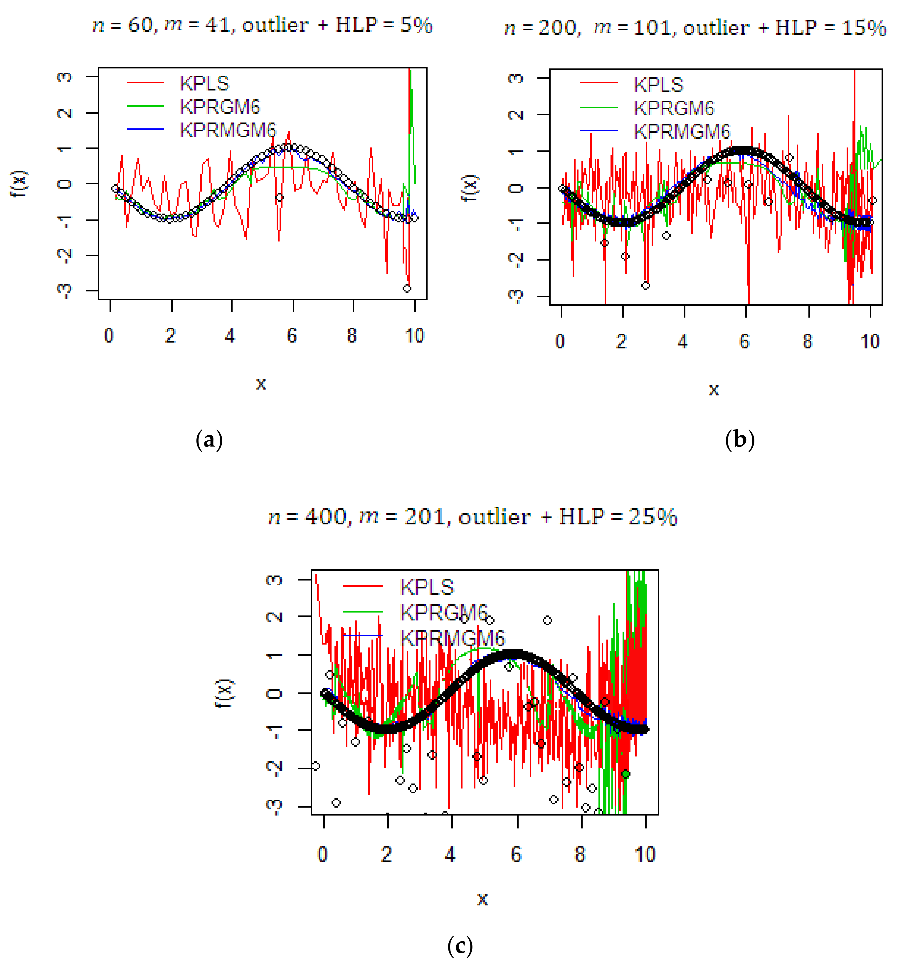
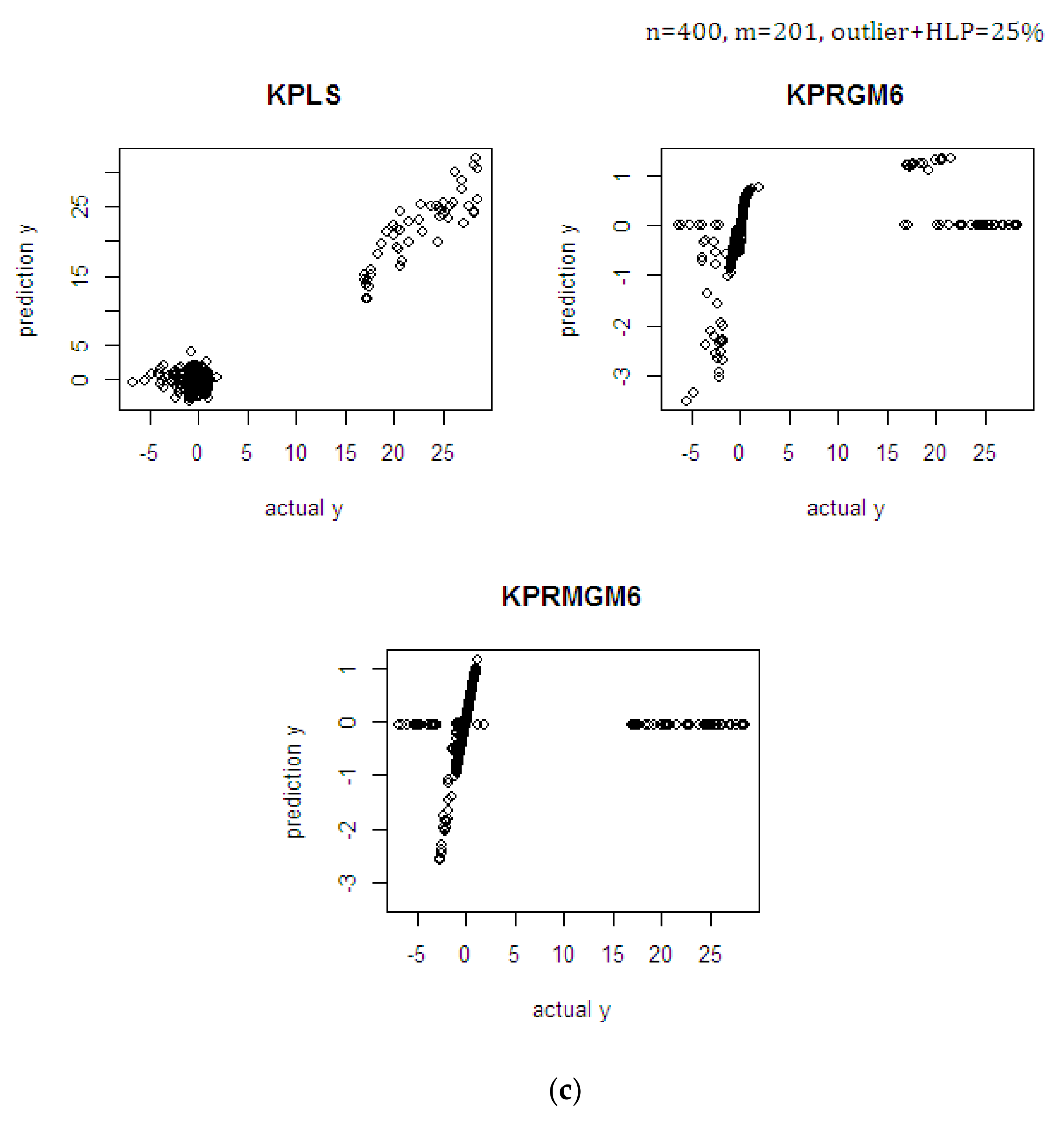
4.1. Monte Carlo Simulation Study

It is known that almost all the available chemometric methods are only capable of capturing linear datasets; however, they fail to capture the structure of highly nonlinear datasets. The artificial data use the $\sin \left(\mathrm{x}\right)$ function [7] to create the nonlinear behavior in the dataset. The artificial dataset is generated randomly using a uniform distribution within the range of $[0,10]$. The scenarios in the simulation use a different artificial dataset that is based on sample size, number of predictors, and level of contamination of outliers and HLPs. The sample size uses $n=$ 40, 60, 160, and 400, while the number of predictor variables uses $m=$ 41, 101, and 201. The different levels $\alpha =$ 0.05, 0.15, and 0.25 of outliers and HLPs were applied to evaluate the robustness. The formulation of this artificial data can be defined as follows:

$$\begin{array}{ll}k = \left\{0,0+d,\left(0+d\right)+d,\dots ,10\right\}& \left(d=1/\left(\right(n-out-h)/10)\right)\\ c_j= k+U\left( 1,10\right)& \left(j=1, 2, 3,\dots ,m\right)\\ e ~ N \left(0,1\right)& \left(i=1, 2, 3,\dots ,n\right)\\ x_j=c_j& \left(j=1, 2, 3,\dots ,m\right)\\ y= \sin \left(-4/5\left(k\right)\right)+e& \left(i=1, 2, 3,\dots ,n\right)\end{array}$$

(19)

where the $c_j$ and $e$ are independent of each other while $x_j$ and $y$ are observable variables. The variable $c_j$ is the sum of the arithmetic sequence $k$ and random values using uniform distribution. The artificial spectra $X$ is the collection of $x_j$, while $y$ uses the sine function, which is calculated through the sum of the sine function of stated initial sequence with added noise $e$. If the sample order is considered as HLPs in $X$ dimension, then $c_j= k+U\left(5,10\right)$. Corresponding to the vertical outlier in $y$, the $y_i= \sin \left(-4/5\left(k\right)\right)-e_i$, while if it is considered as HLP, the $y_i= \sin \left(-4/5\left(k\right)\right)+e_i$, where $e~U\left(3,5\right)$. Clearly, the illustration of the scenarios using this formulation can be seen in Figure 1.

As seen in Figure 1, the illustrations of the scenarios using different level contamination of outliers and HLPs in the dataset are presented in terms of an open circle. In Figure 1a, the scenario uses a small sample size, number of predictors, and level of contaminations. While in Figure 1b,c, the scenarios are set to be higher. These data are assumed good enough to evaluate the nonlinear effects of the proposed methods. We decide not to increase the level contamination of outliers and HLPs greater than 25% since with relating to data acquisition quality, this is not acceptable. The superiority of the proposed methods is evaluated by plotting the prediction values on the original artificial data (see Figure 2). As seen in Figure 2a, using a small sample size, number of predictors, and 5% level contamination, the calibration models with KPRGM6 and KPRMGM6 produce better prediction results than KPLS. This can be observed through the fitted line of predicted values against the actual values in the proposed methods (see the green line and blue line). According to the robustness performance, the KPRMGM6 is superior to KPRGM6. This is because the KPRGM6 suffers the influence of HLPs in the dataset. By increasing the sample size, the number of predictors, and level contaminations (see Figure 2b,c), the proposed KPRMGM6 (blue line) is still superior to the KPRGM6 and KPLS since it almost fits the whole actual values. In general, the kernel solution succeeded in figuring out the nonlinear structure of the dataset. With the contamination of outliers and HLPs in the dataset, the non-robust KPLS suffers from the swamping and masking effects, while the robust KPRGM6 is only able to downgrade partially some of the effects. On the other hand, KPRMGM6 is able to prevent the contamination of both outliers and BLPs; hence, it produces a better fitting line and efficiency. To confirm this finding, the Monte Carlo simulation ran 10,000 simulations, and the results are based on the average of statistical measures.

By preventing the effects of outliers and HLPs in the fitting process (see

Table A1. Statistical measures in kernel partial methods using the sine function.

Outliers and HLPs	n	m	Methods	RMSE	R2	SE
With outliers and HLPs (5%)	60	41	KPLS	2.933	0.523	2.957
			KPRGM6	0.458	0.706	0.462
			KPRMGM6	0.140	0.921	0.140
	60	101	KPLS	2.985	0.515	3.010
			KPRGM6	0.477	0.640	0.481
			KPRMGM6	0.142	0.912	0.142
	60	201	KPLS	3.051	0.522	3.077
			KPRGM6	0.500	0.658	0.504
			KPRMGM6	0.098	0.932	0.101
	200	41	KPLS	2.778	0.438	2.785
			KPRGM6	0.422	0.663	0.423
			KPRMGM6	0.120	0.910	0.120
	200	101	KPLS	2.701	0.430	2.707
			KPRGM6	0.393	0.688	0.394
			KPRMGM6	0.123	0.909	0.124
	200	201	KPLS	2.762	0.429	2.769
			KPRGM6	0.391	0.652	0.392
			KPRMGM6	0.163	0.895	0.163
	400	41	KPLS	2.830	0.418	2.834
			KPRGM6	0.383	0.702	0.384
			KPRMGM6	0.198	0.814	0.200
	400	101	KPLS	2.772	0.421	2.775
			KPRGM6	0.415	0.674	0.416
			KPRMGM6	0.122	0.910	0.122
	400	201	KPLS	2.855	0.427	2.859
			KPRGM6	0.352	0.712	0.353
			KPRMGM6	0.104	0.959	0.104
With outliers and HLPs (15%)	60	41	KPLS	3.456	0.560	3.485
			KPRGM6	0.559	0.620	0.563
			KPRMGM6	0.187	0.859	0.189
	60	101	KPLS	3.459	0.564	3.488
			KPRGM6	0.553	0.700	0.558
			KPRMGM6	0.187	0.860	0.189
	60	201	KPLS	3.484	0.580	3.513
			KPRGM6	0.504	0.664	0.508
			KPRMGM6	0.125	0.930	0.126
	200	41	KPLS	3.533	0.592	3.542
			KPRGM6	0.572	0.736	0.573
			KPRMGM6	0.214	0.841	0.215
	200	101	KPLS	3.359	0.597	3.368
			KPRGM6	0.532	0.672	0.533
			KPRMGM6	0.139	0.898	0.139
	200	201	KPLS	3.330	0.602	3.338
			KPRGM6	0.493	0.707	0.495
			KPRMGM6	0.171	0.872	0.172
	400	41	KPLS	3.505	0.589	3.510
			KPRGM6	0.589	0.662	0.590
			KPRMGM6	0.217	0.815	0.218
	400	101	KPLS	3.529	0.619	3.534
			KPRGM6	0.515	0.645	0.515
			KPRMGM6	0.195	0.807	0.196
	400	201	KPLS	3.405	0.639	3.409
			KPRGM6	0.525	0.658	0.526
			KPRMGM6	0.138	0.851	0.139
With outliers and HLPs (25%)	60	41	KPLS	3.585	0.676	3.615
			KPRGM6	0.749	0.696	0.755
			KPRMGM6	0.131	0.899	0.132
	60	101	KPLS	3.535	0.642	3.565
			KPRGM6	0.680	0.670	0.686
			KPRMGM6	0.248	0.872	0.250
	60	201	KPLS	3.471	0.687	3.501
			KPRGM6	0.464	0.694	0.468
			KPRMGM6	0.154	0.843	0.155
	200	41	KPLS	3.672	0.586	3.681
			KPRGM6	0.653	0.640	0.655
			KPRMGM6	0.240	0.749	0.241
	200	101	KPLS	3.779	0.680	3.789
			KPRGM6	0.616	0.754	0.618
			KPRMGM6	0.136	0.896	0.137
	200	201	KPLS	3.722	0.681	3.731
			KPRGM6	0.591	0.717	0.592
			KPRMGM6	0.252	0.855	0.253
	400	41	KPLS	3.646	0.633	3.651
			KPRGM6	0.641	0.657	0.642
			KPRMGM6	0.248	0.755	0.249
	400	101	KPLS	3.616	0.686	3.621
			KPRGM6	0.578	0.694	0.579
			KPRMGM6	0.236	0.771	0.236
	400	201	KPLS	3.679	0.684	3.684
			KPRGM6	0.559	0.720	0.559
			KPRMGM6	0.224	0.785	0.225

), the KPRMGM6 produces the lowest prediction error (RMSE) and better R² than KPRGM6 and KPLS. The KPLS still suffers from the swamping effects in the fitting process. The KPRGM6 only partially succeeds in removing the influence of outliers and BLPs in the dataset. Using different scenarios, even with low and high levels of contaminations applied in the fitting process, the results using the KPRMGM6 are still satisfactory. Clear outliers and HLPs in the dataset can be observed in Figure 3. In Figure 3a, using small sample size, number of predictors, and 5% level contamination, the KPLS really suffers from the outliers and HLPs in the dataset. This has a dramatic impact to mislead the fitted model, making the accuracy of the model low. The KPRGM6 is only able to partially downgrade the effect of contamination, which leads to a decrease in the accuracy of the fitted model. Using a higher level of contaminations (15% and 25%), the KPRGM6 still suffers from the influence, which increases the prediction error; in addition, the accuracy in KPLS becomes worse (see Figure 3b,c). Here, the fitted regression line using KPRMGM6 shows better performance (efficiency and accuracy) than the KPRGM6 and KPLS since the model is not really affected by the contamination of outliers and BLPs.

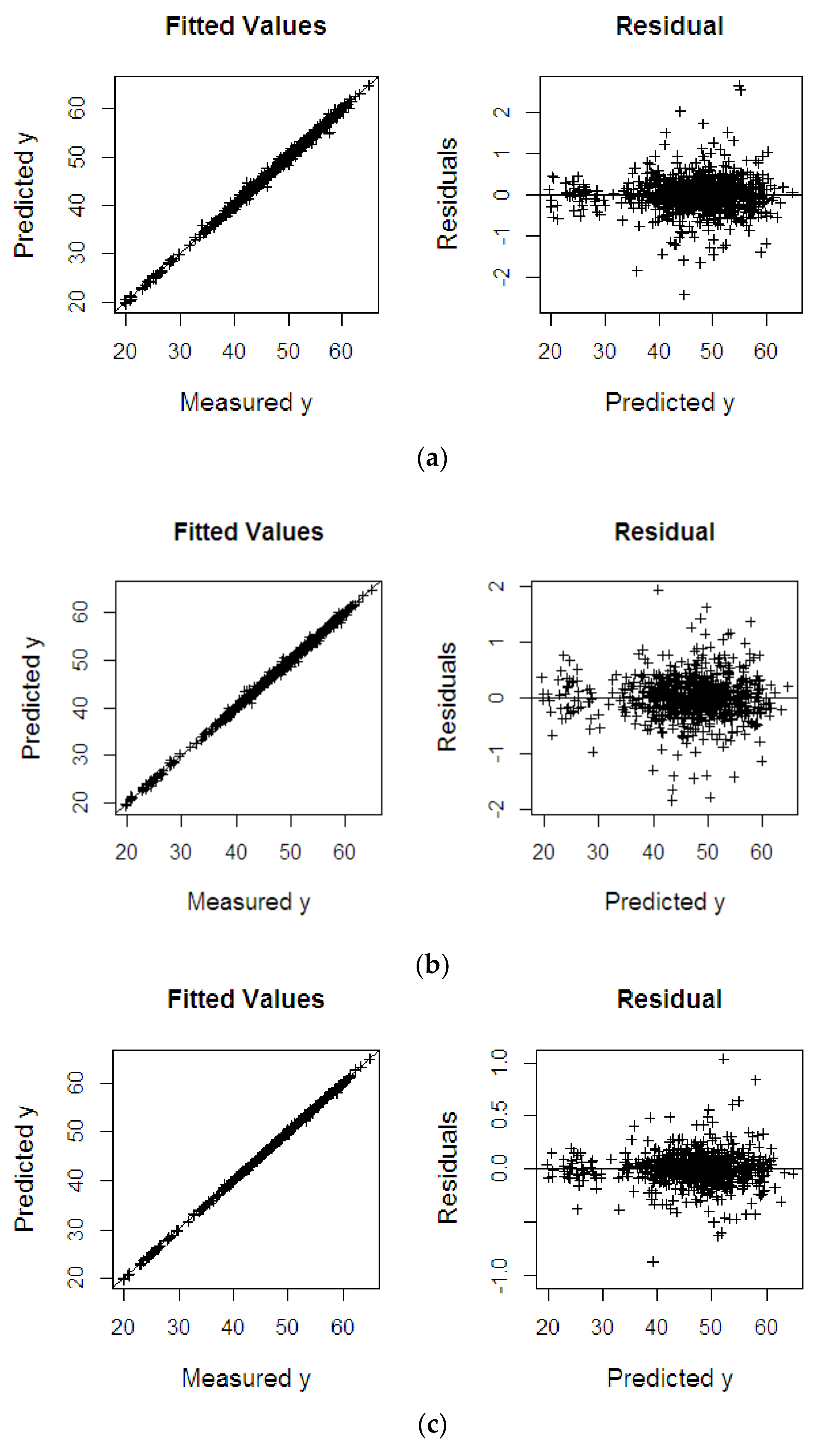
4.2. NIR Spectral Data

The spectral data use light absorbance in each $j$ wavelength band adopted from the Beer–Lambert law [36], and the data are presented in $m\times 1$ column vector $x_j$ using the log base 10. The spectral measurement was obtained by scanning (in contact) the fruit mesocarp using a portable handheld NIR spectrometer (QualitySpec Trek) from Analytical Spectral Devices (ASD Inc., Boulder, Colorado (CO), USA). A total of 80 fruit bunches were harvested from the site of the breeding trial in Palapa Estate, PT. Ivomas Tunggal, Riau Province, Indonesia. In a bunch, there were 12 fruit mesocarp samples collected from different sampling positions. The sampling positions comprised the vertical and horizontal lines in a bunch [37]: bottom-front, bottom-left, bottom-back, bottom-right, equator-front, equator-left, equator-back, equator-right, top-front, top-left, top-back, and top-right. Right after the collection, the fruit mesocarp samples were sent immediately to the laboratory for spectral measurement and wet chemistry analysis. The sources of variability such as planting materials (Dami Mas, Clone, Benin, Cameroon, Angola, Colombia), planting year (2010, 2011, 2012), and ripeness level (unripe, under-ripe, ripe, over-ripe) were also considered to cover the different sources of variation in the palm population as much as possible.

Two sets of NIR spectral data with different sample properties of fruit mesocarp (fresh and dried ground) were used. The average of three spectra measurements of each fruit sample mesocarp was used in the computation. The fresh fruit mesocarp was used to estimate the %ODM and %OWM, while the dried ground mesocarp was used to estimate the %FFA. These parameters were analyzed through conventional analytical chemistry that adopts standard test methods from the Palm Oil Research Institute of Malaysia (PORIM) [38,39]. The %ODM was calculated on a dry matter basis, which removes the weight of water content, while the %OWM used a wet matter basis. Statistically, the distribution range of %ODM used as the dataset is 56.38–86.9%; the %OWM is 19.75–64.81%; and the %FFA is 0.17–6.3%. The NIR spectra on oil palm fruit mesocarp (both in fresh and dried ground mesocarp) and its frequency distribution on response variables, the %ODM, %OWM, and %FFA, can be seen in the previous study [37]. It is important to note that there is no prior knowledge on whether outliers and HLPs are present in this dataset. Therefore, the methods were evaluated based on their accuracy improvement through its desirability index.

4.2.1. Oil to Dry Mesocarp

The NIR spectra of fresh fruit mesocarp from 960 observations involving 488 wavelengths (range 550–2500 nm: 4 nm interval) were used in this study. Using the %ODM as the response variable, the effectiveness of the proposed methods was presented. As seen in

Table 1. Statistical measures on the prediction results using %ODM, %OWM, and %FFA datasets.

Dataset	Methods	RMSEP	R2	SE
%ODM	KPLS	0.283	0.927	0.282
	KPRGM6	0.250	0.997	0.252
	KPRMGM6	0.128	0.999	0.128
%OWM	KPLS	0.404	0.967	0.402
	KPRGM6	0.364	0.998	0.365
	KPRMGM6	0.301	0.999	0.301
%FFA	KPLS	0.222	0.814	0.222
	KPRGM6	0.207	0.844	0.208
	KPRMGM6	0.117	0.866	0.117

, the robust KPRMGM6 improves the accuracy of the model with the lowest prediction error (0.128) and better R² (0.999) than the KPRGM6 and KPLS. The non-robust KPLS produces higher SE (0.282–0.283) with lower R² (0.927) compared to the KPRGM6 and KPRMGM6. It is known that the proposed robust methods are able to prevent the influence of outliers and HLPs in the dataset; thus, they produce more accurate predictions. The comparison between the measured and predicted values is presented in the fitting line regression (see Figure 4). It shows that by using the proposed robust methods (see Figure 4b,c), the model predictions have been able to approximately estimate the measured values. The robust KPRMGM6 fits the data more accurately compared to the robust KPRGM6. Corresponding to the residual plots produced by the proposed methods, the KPRMGM6 (see Figure 4c) yields the lowest prediction error than the remaining methods.

4.2.2. Oil to Wet Mesocarp

Using a similar NIR spectral dataset as in the previous analysis, %OWM was used as a response variable. As seen in Table 1, it is known that the proposed robust KPRGM6 and KPRMGM6 are still superior to the non-robust KPLS. This is because the KPLS fails to prevent the influence of outliers and HLPs that may exist in the dataset. The two robust methods produce better R² (0.998–0.999) and lower prediction error (0.301–0.364). Based on these results, the KPRGM6 and KPRMGM6 are still superior as they show their robustness compared to the non-robust KPLS. The visual comparison between the measured values against the predicted values of the two proposed robust methods can be seen in Figure 5. It is observed that both the KPRGM6 and KPRMGM6 have successfully fit the measured values adequately with less error (see Figure 5b,c). However, the KPRMGM6 still outperforms the KPRGM6. As highlighted in the residual plots, the KPRMGM6 yields the lowest prediction error (see Figure 5c) compared to KPRGM6, which is dominantly close to 0. Hence, the results confirm our previous claims. In this study, even though the same NIR spectral data are used as predictor variables, with the different use of response variables, the desirability indices show different results. Nonetheless, the summarized performance of the two proposed robust methods remains satisfactory.

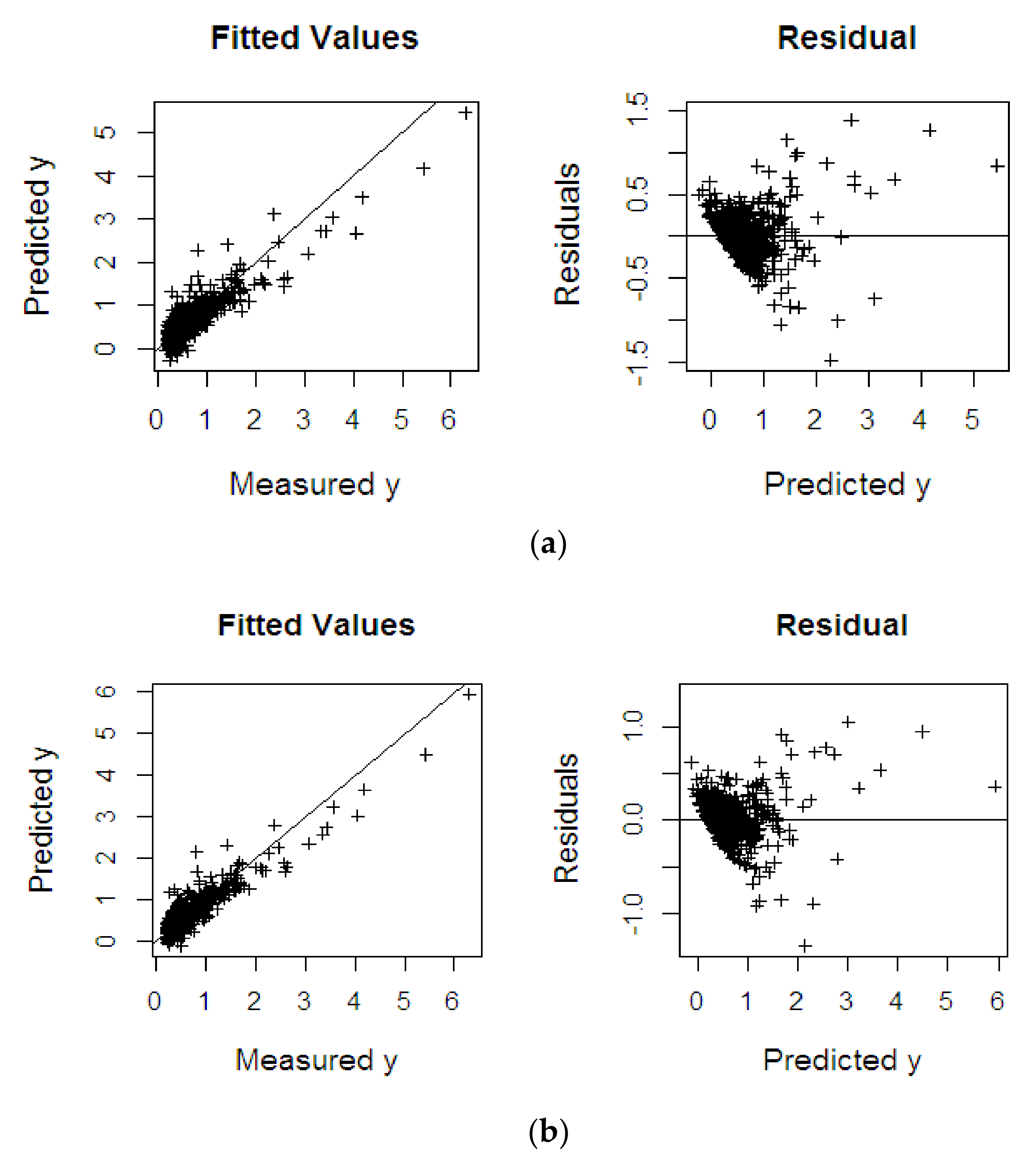
4.2.3. Fat Fatty Acids

Another set of NIR spectra of dried ground mesocarp from 839 observations and 500 wavelengths (range 500–2500 nm: 4 nm interval) was used in the study. Here, the %FFA was used as the response variable. As seen in Table 1, the two proposed robust KPRGM6 and KPRMGM6 are better than non-robust KPLS as it yields the highest error in the prediction (0.222) and the lowest R² (0.814). The robust procedures in KPRGM6 and KPRMGM6 have prevented the PLSR model from the influence of outliers and HLPs that may exist in the dataset. Based on the fitted regression line graphs (see Figure 6), the KPRGM6 and KPRMGM6 models summarize the variability (84.4–86.6%) of the response data adequately. As seen in the residual plot (see Figure 6b,c), the KPRMGM6 produces less error (0.117) than KPRGM6 (0.207). It also observed that there is no specific pattern shown in the residual plot both in KPRGM6 and KPRMGM6; this claims a good fit of predicted values that are a random pattern. With robust procedures provided in the PLSR model, this model is relatively good enough to be used in further interpretation since it is resistant to the influence of outliers and BLPs. The range of %FFA data used in the calibration model is still needed to be expanded in order to guarantee all the possible outcome values are covered in the model. In general, we measure the %FFA using the conventional laboratory method, which is based on the extracted oil from ground dried mesocarp. This then would contribute to increasing the bias in the model accuracy of the proposed method.

5. Conclusions

With consideration to the high dimensionality and irregular data space in the dataset, particularly for chemometric analysis on NIR spectral data, the two new robust methods called the KPRGM6 and KPRMGM6 algorithms are proposed. The methods combine the benefits of linear PLSR and the kernel-based learning RHKS with the robustness of the modified GM6 estimators. Based on the results, the proposed robust methods have generally succeeded in preventing the influence of outliers and HLPs in the dataset and captured the nonlinear relationships through high-dimensional feature mapping. The non-robust KPLS suffers from the contamination of outliers and HLPs; hence, it has decreased the accuracy of the PLS model. In the investigation, the use of different datasets reached different desirability indexes where the KPRMGM6 is generally superior to KPRGM6 in terms of accuracy improvement. The proposed modified KPRMGM6 shows its superiority by removing only the outliers and BLPs in the dataset since GLPs contribute to increasing the efficiency during the fitting process of parameter estimates. By adding some artificial outliers and HLPs in the Monte Carlo simulation data, the KPRGM6 has only managed to detect some outliers while the rest are unidentified. On the other hand, the contamination of all real outliers and BLPs in the dataset has to be down-weighted for the proposed KPRMGM6 to show great prominence. For future research, combining the proposed KPRMGM6 with the robust pre-processing and wavelength selection method is highly suggested. This will contribute to creating a more flexible, robust PLSR method rather than applying the method separately. A consideration to employing such machine learning (ML) and deep learning (DL) methods to figure out the nonlinear behavior in the dataset is also encouraged.

References

1. Midi, H.; Norazan, M.; Imon, A.H.M. The performance of diagnostic-robust generalized potentials for the identification of multiple high leverage points in linear regression. J. Appl. Stat. 2009, 36, 507–520. [Google Scholar]
2. Bagheri, A.; Midi, H. Diagnostic plot for the identification of high leverage collinearity-influential observations. Sort Stat. Oper. Res. Trans. 2015, 39, 51–70. [Google Scholar]
3. Alguraibawi, M.; Midi, H.; Imon, A.H.M. A new robust diagnostic plot for classifying good and bad high leverage points in a multiple linear regression model. Math. Probl. Eng. 2015, 2015, 1–12. [Google Scholar] [CrossRef]
4. Atkinson, A.C. Fast very robust methods for the detection of multiple outliers. J. Am. Stat. Assoc. 1994, 89, 1329–1339. [Google Scholar] [CrossRef]
5. Imon, A.H.M. Identifying multiple high leverage points in linear regression. J. Stat. Stud. 2002, 3, 207–218. [Google Scholar]
6. Serneels, S.; Croux, C.; Filzmoser, P.; Van Espen, P.J. Partial robust M-regression. Chemom. Intell. Lab. Syst. 2005, 79, 55–64. [Google Scholar] [CrossRef]
7. Jia, R.D.; Mao, Z.Z.; Chang, Y.Q.; Zhang, S.N. Kernel partial robust M-regression as a flexible robust nonlinear modeling technique. Chemom. Intell. Lab. Syst. 2010, 100, 91–98. [Google Scholar] [CrossRef]
8. Wold, H. Multivariate Analysis; Krishnaiah, P.R., Ed.; Academic Press: New York, NY, USA, 1973; Volume 3, pp. 383–407. [Google Scholar]
9. Rosipal, R. Nonlinear partial least squares an overview. In Chemoinformatics and Advanced Machine Learning Perspectives: Complex Computational Methods and Collaborative Techniques; IGI Global: Hershey, PA, USA, 2011; pp. 169–189. [Google Scholar]
10. Yang, H.; Griffiths, P.R.; Tate, J.D. Comparison of partial least squares regression and multi-layer neural networks for quantification of nonlinear systems and application to gas phase Fourier transform infrared spectra. Anal. Chim. Acta 2003, 489, 125–136. [Google Scholar] [CrossRef]
11. Balabin, R.M.; Safieva, R.Z.; Lomakina, E.I. Comparison of linear and nonlinear calibration models based on near infrared (NIR) spectroscopy data for gasoline properties prediction. Chemom. Intell. Lab. Syst. 2007, 88, 183–188. [Google Scholar] [CrossRef]
12. Schölkopf, B.; Smola, A.; Müller, K.R. Nonlinear component analysis as a kernel eigenvalue problem. Neural Comput. 1998, 10, 1299–1319. [Google Scholar] [CrossRef] [Green Version]
13. Rosipal, R.; Trejo, L.J. Kernel partial least squares regression in reproducing kernel hilbert space. J. Mach. Learn. Res. 2001, 2, 97–123. [Google Scholar]
14. Bennett, K.P.; Embrechts, M.J. An optimization perspective on kernel partial least squares regression. Nato Sci. Ser. Sub Ser. Iii Comput. Syst. Sci. 2003, 190, 227–250. [Google Scholar]
15. Sindhwani, V.; Minh, H.Q.; Lozano, A.C. Scalable matrix-valued kernel learning for high-dimensional nonlinear multivariate regression and Granger Causality. In Proceedings of the Twenty-Ninth Conference on Uncertainty in Artificial Intelligence, Bellevue, WA, USA, 11–15 August 2013; pp. 586–595. [Google Scholar]
16. Ma, X.; Zhang, Y.; Cao, H.; Zhang, S.; Zhou, Y. Nonlinear regression with high-dimensional space mapping for blood component spectral quantitative analysis. J. Spectrosc. 2018, 1–8. [Google Scholar] [CrossRef] [Green Version]
17. Aronszajn, N. Theory of reproducing kernels. Trans. Am. Math. Soc. 1950, 68, 337–404. [Google Scholar] [CrossRef]
18. Preda, C. Regression models for functional data by reproducing kernel Hilbert spaces methods. J. Stat. Plan. Inference 2007, 137, 829–840. [Google Scholar] [CrossRef]
19. Coakley, C.W.; Hettmansperger, T.P. A bounded influence, high breakdown, efficient regression estimator. J. Am. Stat. Assoc. 1993, 88, 872–880. [Google Scholar] [CrossRef]
20. Rousseeuw, P.J. Regression techniques with high breakdown point. Inst. Math. Stat. Bull. 1983, 12, 155. [Google Scholar]
21. Rousseeuw, P.J. Multivariate estimation with high breakdown point. In Mathematical Statistics and Applications; Grossmann, W., Pflug, G., Vincze, I., Wertz, W., Eds.; Cengage Learning: Belmont, CA, USA, 1985; Volume 37, pp. 283–297. [Google Scholar]
22. Rousseeuw, P.J.; Leroy, A.M. Robust Regression and Outlier Detection. In Wiley Series in Probability and Mathematical Statistics: Applied Probability and Statistics; Wiley: New York, NY, USA, 1987. [Google Scholar]
23. Rousseeuw, P.J. Least median of squares regression. J. Am. Stat. Assoc. 1984, 79, 871–880. [Google Scholar] [CrossRef]
24. Midi, H. Robust Estimation of a Linearized Nonlinear Regression Model with Heteroscedastic Errors: A Simulation Study. Pertanika J. Sci. Technol. 1998, 6, 23–35. [Google Scholar]
25. De Haan, J.; Sturm, J.-E. No Need to Run Millions of Regressions. Available at SSRN 246453 2000, 1–12. Available online: https://papers.ssrn.com/sol3/papers.cfm?abstract_id=246453 (accessed on 13 October 2020).
26. Midi, H.; Hendi, H.T.; Arasan, J.; Uraibi, H. Fast and Robust Diagnostic Technique for the Detection of High Leverage Points. Pertanika J. Sci. Technol. 2020, 28, 1203–1220. [Google Scholar] [CrossRef]
27. Silalahi, D.D.; Midi, H.; Arasan, J.; Mustafa, M.S.; Caliman, J.P. Kernel partial diagnostic robust potential to handle high-dimensional and irregular data space on near infrared spectral data. Heliyon 2020, 6, 1–12. [Google Scholar] [CrossRef] [PubMed]
28. Lim, H.A.; Midi, H. Diagnostic Robust Generalized Potential Based on Index Set Equality (DRGP (ISE)) for the identification of high leverage points in linear model. Comput. Stat. 2016, 31, 859–877. [Google Scholar] [CrossRef]
29. Minasny, B.; McBratney, A. Why you don’t need to use RPD. Pedometron 2013, 33, 14–15. [Google Scholar]
30. Rännar, S.; Lindgren, F.; Geladi, P.; Wold, S. A PLS kernel algorithm for data sets with many variables and fewer objects. Part 1: Theory and algorithm. J. Chemom. 1994, 8, 111–125. [Google Scholar] [CrossRef]
31. Wold, H. Soft modelling by latent variables: The non-linear iterative partial least squares (NIPALS) approach. J. Appl. Probab. 1975, 12, 117–142. [Google Scholar] [CrossRef]
32. Cummins, D.J.; Andrews, C.W. Iteratively reweighted partial least squares: A performance analysis by Monte Carlo simulation. J. Chemom. 1995, 9, 489–507. [Google Scholar] [CrossRef]
33. Huber, P.J. Robust regression: Asymptotics, conjectures and Monte Carlo. Ann. Stat. 1973, 1, 799–821. [Google Scholar] [CrossRef]
34. Rousseeuw, P.J.; Driessen, K.V. A fast algorithm for the minimum covariance determinant estimator. Technometrics 1999, 41, 212–223. [Google Scholar] [CrossRef]
35. Rousseeuw, P.J.; Croux, C. Alternatives to the median absolute deviation. J. Am. Stat. Assoc. 1993, 88, 1273–1283. [Google Scholar] [CrossRef]
36. Stuart, B. Infrared Spectroscopy: Fundamentals and Applications; Wiley: Toronto, ON, Canada, 2004; pp. 167–185. [Google Scholar]
37. Silalahi, D.D.; Midi, H.; Arasan, J.; Mustafa, M.S.; Caliman, J.P. Robust Wavelength Selection Using Filter-Wrapper Method and Input Scaling on Near Infrared Spectral Data. Sensors 2020, 20, 5001. [Google Scholar] [CrossRef] [PubMed]
38. Siew, W.L.; Tan, Y.A.; Tang, T.S. Methods of Test for Palm Oil and Palm Oil Products: Compiled; Lin, S.W., Sue, T.T., Ai, T.Y., Eds.; Palm Oil Research Institute of Malaysia: Selangor, Malaysia, 1995. [Google Scholar]
39. Rao, V.; Soh, A.C.; Corley, R.H.V.; Lee, C.H.; Rajanaidu, N. Critical Reexamination of the Method of Bunch Quality Analysis in Oil Palm Breeding; PORIM Occasional Paper; FAO: Rome, Italy, 1983; Available online: https://agris.fao.org/agris-search/search.do?recordID=US201302543052 (accessed on 13 October 2020).
Figure 1. Training dataset using sine function with different scenarios: (a) n = 60, m = 41, outliers + high leverage points (HLPs) = 5%; (b) n = 200, m = 101, outliers + HLPs = 15%; (c) n = 400, m = 201, outliers + HLPs = 25%.
Symmetry 13 00547 g001
Figure 2. Predictions on artificial data using the calibration model of kernel partial least square (KPLS), kernel partial robust GM6-estimator (KPRGM6), and kernel partial robust modified GM6-estimator (KPRMGM6) on different dataset scenarios: (a) n = 60, m = 41, outliers + HLPs = 5%; (b) n = 200, m = 101, outliers + HLPs = 15%; (c) n = 400, m = 201, outliers + HLPs = 25%.
Symmetry 13 00547 g002
Figure 3. Actual values against predicted values on different dataset scenarios: (a) n = 60, m = 41, outliers + HLPs = 5%; (b) n = 200, m = 101, outliers + HLPs = 15%; (c) n = 400, m = 201, outliers + HLPs = 25%.
Symmetry 13 00547 g003aSymmetry 13 00547 g003b
Figure 4. Measured values against predicted values and the residual using %ODM data: (a) KPLS, (b) KPRGM6, and (c) KPRMGM6.
Symmetry 13 00547 g004
Figure 5. Measured values against predicted values and the residual using %OWM data: (a) KPLS, (b) KPRGM6, and (c) KPRMGM6.
Symmetry 13 00547 g005
Figure 6. Measured values against predicted values and the residual using %FFA data: (a) KPLS, (b) KPRGM6, and (c) KPRMGM6.
Symmetry 13 00547 g006aSymmetry 13 00547 g006b