
Financial Information Asymmetry: Using Deep Learning Algorithms to Predict Financial Distress

Department of Accounting, Soochow University, No.56, Section 1, Kueiyang Street, Chungcheng District, Taipei 10048, Taiwan
Symmetry 2021, 13(3), 443; https://doi.org/10.3390/sym13030443
Submission received: 10 February 2021
/
Revised: 1 March 2021
/
Accepted: 4 March 2021
/
Published: 9 March 2021
Abstract
:Because of the financial information asymmetry, the stakeholders usually do not know a company’s real financial condition until financial distress occurs. Financial distress not only influences a company’s operational sustainability and damages the rights and interests of its stakeholders, it may also harm the national economy and society; hence, it is very important to build high-accuracy financial distress prediction models. The purpose of this study is to build high-accuracy and effective financial distress prediction models by two representative deep learning algorithms: Deep neural networks (DNN) and convolutional neural networks (CNN). In addition, important variables are selected by the chi-squared automatic interaction detector (CHAID). In this study, the data of Taiwan’s listed and OTC sample companies are taken from the Taiwan Economic Journal (TEJ) database during the period from 2000 to 2019, including 86 companies in financial distress and 258 not in financial distress, for a total of 344 companies. According to the empirical results, with the important variables selected by CHAID and modeling by CNN, the CHAID-CNN model has the highest financial distress prediction accuracy rate of 94.23%, and the lowest type I error rate and type II error rate, which are 0.96% and 4.81%, respectively.
1. Introduction
In the latter half of 2008, the subprime mortgage crisis in the United States continued and spread worldwide, triggering a global financial crisis and affecting the global economy. Accordingly, many companies were in serious financial distress, including companies in Taiwan. Impacted by the subprime mortgage of the United States, in 2008, the Indy Mac Bank was in financial distress, and was taken over by the Federal Deposit Insurance Corporation of the U.S. government, Lehman Brothers declared bankruptcy, and the American International Group (AIG) applied to the Federal Reserve Board (FRD) for emergency financing of USD 85 billion. In 2009, Merrill Lynch was acquired by the Bank of America, and later, the financial tsunami swept the world. Taiwan is not immune. The Financial Supervisory Commission declared the take-over of many financial institutions in financial distress, including the Chinfon Commercial Bank (Note: Chinfon Commercial Bank was later merged to create the Far Eastern International Bank and Yuanta Commercial Bank, respectively). Taiwan’s economy was hit very hard [1], and many companies and factories closed, leaving employees jobless and investors with nothing. The global financial crisis of 2008 showed that financial crises can happen even to strong international companies, thus, they must be constantly vigilant about their finances positions [2]. Moreover, due to the impact of the global financial crisis, the number of companies going bankrupt rose sharply in many countries, and the importance of financial distress prediction models also increased [3], which was of great significance for corporate sustainable development.
According to some studies, financial distress is usually caused by poor financial structures. The financial leverage of a company will increase its agency costs and lead managers to be more likely to make high risk decisions [4,5,6], and poor financial structures are usually inversely related to corporate performance [7]. While companies’ operating condition are regularly disclosed in their financial statements, in general, due to information asymmetry, investors in a company often do not know that the company may be in financial distress until its official financial statement is issued. If company executives deliberately glamorize or falsify financial statements to conceal actual operating or financial conditions, investors will have less opportunity to obtain true financial information; for example, companies can create the illusion that there will be no capital shortage in the short-term by manipulating their current ratios to 200% [8]. As an integral part of financial-economic analysis, predicting the risks of financial distress can help investors and creditors to reveal corporate performance stability. Moreover, based on the consideration of national conditions, the appropriate use of financial prediction indices and statistical approaches can obtain prediction results to predict future corporate development as accurately as possible [9].
Corporate operational quality and the social pulse are inseparable. Corporate operational crisis will cause a growing feeling of insecurity and upset, which leads to a terrible cost to the entire economic environment [10]. Corporate financial distress will directly damage the interests of stakeholders and cause the entire country and society to pay a huge price [11]. From the perspective of corporate survival factors, Sharma and Mahajan [12] pointed out that there are two factors influencing corporate crisis: (1) External factors beyond the control of companies, which refers to the overall environment and industrial profitability; (2) internal factors of companies, which refers to corporate use of resources, such as marketing strategy planning, execution, and supervision. Operators must control their corporate financial risks, as well as the macro economy and regulations of the market in the location where their companies operate [13]. As the core of corporate operations, effective financial management shall be able to predict possible financial distress [14]. As financial distress prediction reveals potential financial deficiencies or risks, they can improve investors’ decision-making, assist financial institutions in their loan decisions, and help regulatory authorities to formulate regulations. If competent authorities, corporate governing bodies, CPAs, auditors, and top management can identify the risk warnings or problems as early as possible, relevant measures may take to prevent the occurrence of distress or deterioration; therefore, effective financial distress prediction is very important [15,16,17,18,19,20]. Generally, in cases of corporate financial distress, there will be some special signs revealed in the process. There are three stages in the period before financial distress: (1) Sharp decline of net cash flow, (2) capital shortage, and (3) the occurrence of financial distress. If the problems remain unresolved during the initial financial distress, companies may liquidate, go bankrupt, fail, or be taken over by others.
While there is a large amount of research literature on corporate financial distress prediction, as the discussion and prediction of financial distress are very important for the overall economy, society, and corporate stakeholders, the issue is worthy of further discussion. This study constructs accurate financial distress prediction models with deep learning methods, including deep neural networks (DNN) and convolutional neural networks (CNN), in order to provide reference for academic research and all circles. In addition, the chi-squared automatic interaction detector (CHAID) is also adopted in this study to select important variables. Now is the era of artificial intelligence (AI), and deep learning algorithms are used in academic research. So far, quite a few studies have used deep learning algorithms to predict financial distress. This study uses a more innovative approach with deep learning algorithms in financial distress research. Therefore, this study hopes to be able to promote the expansion of academic literature and the practice of financial distress prediction.
2. Related Works
Regarding the “information asymmetry”, there is a famous “lemon market” theory in economics, which was proposed in 1970 by Akerlof [21], the Nobel Prize winner in economics in 2001. He pointed out that in a market with “information asymmetry”, when suppliers of goods have more information than buyers, the market shrinks or even disappears. He took the second-hand car market as an example. Because car buyers lack the same information as car sellers, in order to avoid the risk of loss from buying a “bad car”, he is only willing to pay a lower price; this behavior leads to good maintenance. Second-hand car owners are unwilling to send their cars to this market, so the second-hand car market is full of substandard products (commonly known as “lemons” in the United States). Buyers are harming themselves in order to avoid losses. This result is called “adverse selection”. For a market to develop normally, information equivalence between the supply and demand sides is very important; when sufficient information is not available, even if there is demand, it will suppress or find alternatives to avoid losses, resulting in the failure of the market to develop soundly.
The company’s financial condition is also full of financial information asymmetry. The company’s executives hold very different information from others. It is difficult for shareholders, creditors, employees, and other stakeholders to know the true face of the company’s financial condition. It often waits until the company reaches financial distress or bankruptcy.
There are many uses for the financial distress prediction models, including monitoring corporate solvency, assessing the risks of defaults on loans and bonds, pricing credit derivatives, and other securities bearing credit risks [22]. In the 1960s, two famous papers were published which concerned the study of financial distress prediction and the construction of prediction models. One is Beaver’s study in 1966 [23], where corporate financial distress was predicted by univariate analysis, and those with huge bank overdrafts, unpaid dividends on preferred stock, defaults on corporate bonds, and declarations of bankruptcy were defined as companies in financial distress. In that study, companies in financial distress from 1954 to 1964 were taken as samples, another 79 normal companies of similar size and capital in the same industry selected for matching, and 14 financial ratios, such as the ratios measuring profitability, liquidity, and solvency, were selected to predict the possibility of corporate financial distress. According to the results, cash flow/total liabilities was the best in financial distress prediction; however, the univariate model was only able to evaluate one variable at a time and could not consider other company variables as a whole. The other paper was Altman’s study in 1968 [24]. By improving the deficiency of the univariate model, a multivariate differential analysis model was established to predict corporate financial distress. Those legally bankrupt, taken over, or recognized as restructured by the national bankruptcy law were defined as companies in financial distress. In that study, 33 companies in financial distress from 1946 to 1965 were taken as samples, another 33 financially healthy companies with similar assets were selected for matching, and 22 financial ratios were selected from five major comprehensive corporate dimensions, such as liquidity, profitability, financial leverage, solvency, and turnover capacity. Then, the ratios were combined to create a comprehensive index in the Z-Score model: Z = 1.2X1 + 1.4X2 + 3.3X3 +0.6X4 + 1.0X5, where, X1: Working capital/total assets, X2: Retained earnings/total assets, X3: Earnings before interest and taxes/total assets, X4: Market value of equity/book value of total debt, and X5: Sales/total assets. In 2017, Altman et al. predicted financial distress for companies in 31 countries/regions (mostly in Europe) by the Z-Score model, and its accuracy was 70–80% [25].
After the 1960s, in many subsequent studies on financial distress prediction and prediction model construction, multivariate analysis, multiple regression analysis, stepwise regression analysis, and logistic regression methods were used [1,20,26,27,28,29,30,31,32]. However, the strict hypotheses of the models, such as linearity, normality, and independence among the predictive variables of traditional statistics, limited their applications in practice.
In addition to the above traditional financial distress prediction methods, with the rapid development of computers and software technology, data mining and machine learning algorithms were used in many studies about financial distress prediction and prediction model construction [1,8,9,10,33,34,35,36,37,38,39,40]. Among these literature, Chen and Shen [1] use hybrid machine learning methods integrating stepwise regression (SR), the least absolute shrinkage and selection operator (LASSO), classification and regression trees (CART), and random forests (RF) to build the financial distress prediction models. Fourteen financial variables and 6 non-financial variables are used, and the CART-LASSO model has the highest accuracy rate of 89.74% in their study. Chen and Du [8] use neural networks and data mining clustering approach for the financial distress prediction. Thirty-three financial variables and 4 non-financial variables are used, and the result of their study shows that the financial distress prediction models developed by the ANN approach obtain better prediction accuracy than the data mining clustering approach. Gregova et al. [9] use logistic regression (LR), random forests (RF), and neural networks (NN) to predict financial distress. Fourteen financial ratios are used, and the NN model has the best performance (AUC) of 0.886. Chen and Jhuang [9] use SR, ANN, CHAID, and C5.0.to build financial distress prediction models. Eighteen financial variables and 3 non-financial variables are used, and the SR-C5.0 model has the highest prediction accuracy rate of 91.65%.
3. Materials and Methods
As a representative algorithm in the family of decision trees, the chi-squared automatic interaction detector (CHAID) can determine branch variables and partitions from the perspective of statistical significance, in order to optimize the branching process of the tree, thus, CHAID has good classification ability and is suitable for important variable selection. Due to their strong abilities in input variable calculation, deep neural networks (DNN) and convolutional neural networks (CNN) can optimize prediction models. Hence, CHAID, DNN, and CNN are used in this study to build financial distress prediction models.
3.1. Chi-Squared Automatic Interaction Detector
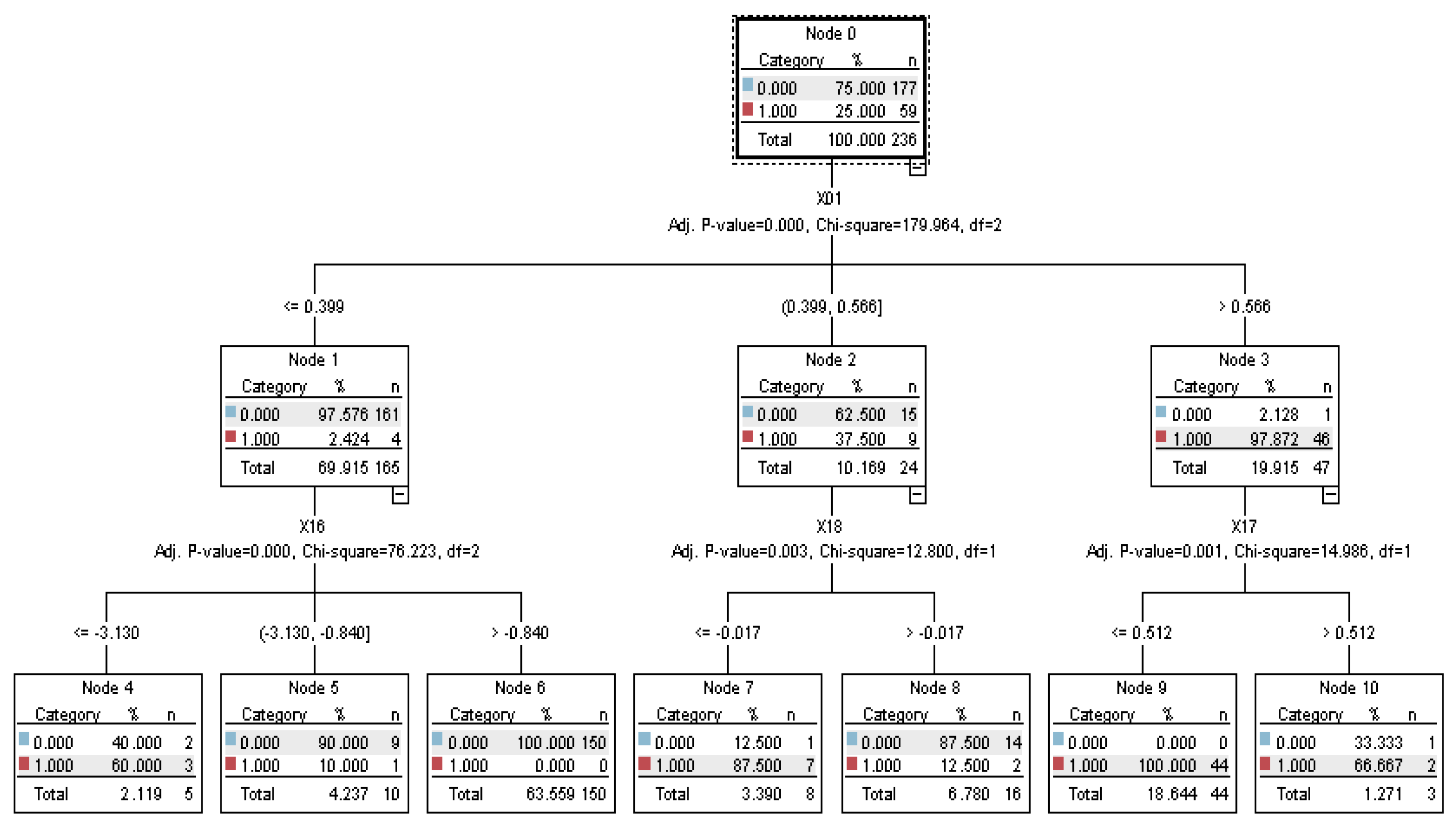
The chi-squared automatic interaction detector (CHAID) is proposed by Kass [41], which is a decision tree algorithm that uses chi-square test statistics and p-values to establish a decision tree, which can identify the relationship between dependent variables and independent variables and deal with the interaction among independent variables. The purpose of chi-square testing is to determine the deviation between the actual observed values and the theoretically inferred values of statistical samples, and the deviation between such values determines the chi-square values. The larger the chi-square value, the greater the deviation; and the smaller the chi-squared value, the smaller the deviation. CHAID can produce non-binary tree structures, which indicates that some partitions have more than two branches; hence, CHAID will build wider tree structures than the binary growth approach. CHAID is also suitable for all types of inputs, and accepts both weighted observed values and frequency variables. When being applied to classification, CHAID can classify data into two or more categories by chi-square testing. In order to determine the optimal partition at any node, this model combines non-significant variables into a similar group until there is no statistically significant difference among the dependent variables in the group. The classification structure of CHAID is shown in Figure 1.
3.2. Deep Neural Networks
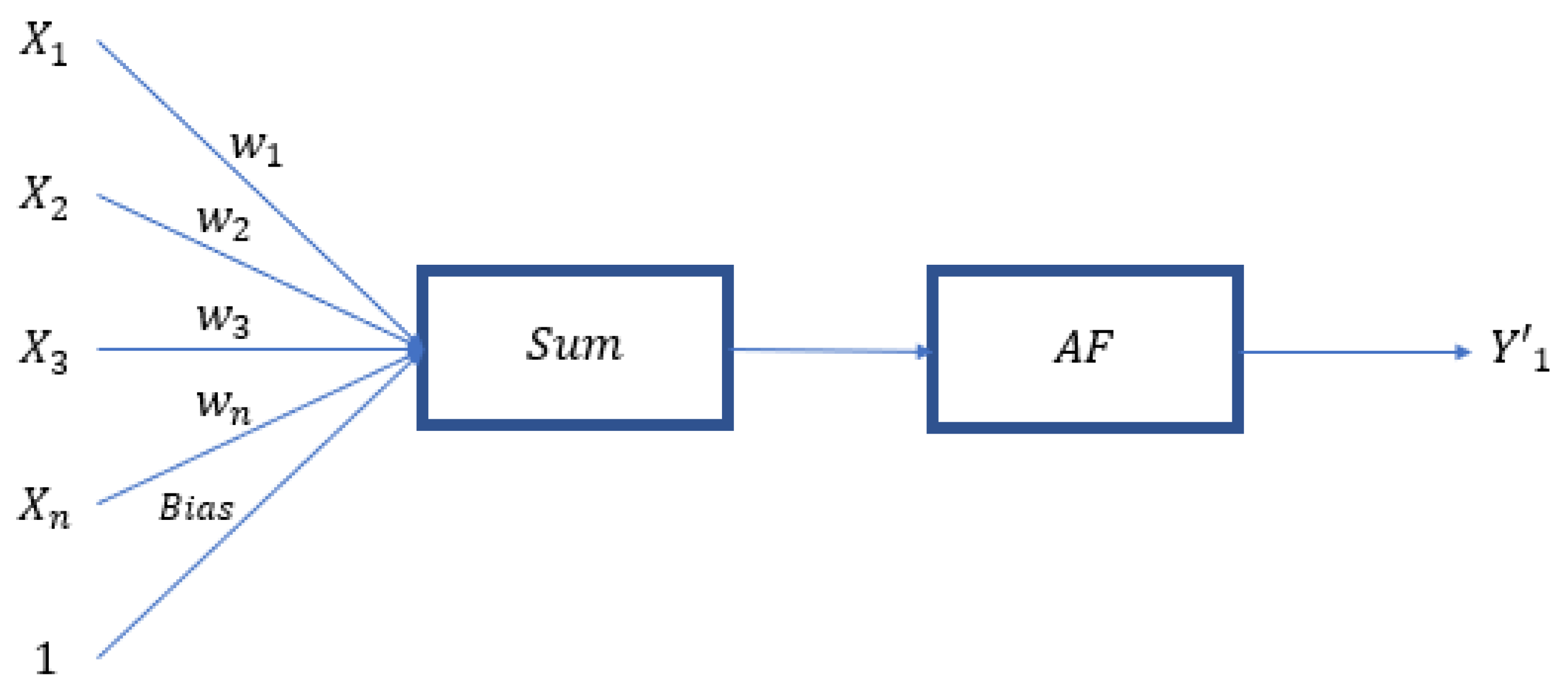
The deep neural network (DNN), which is a deep learning model developed from the artificial neural network, is an artificial neural network with multiple hidden layers, and has the purpose of simulating neurotransmissions in the human brain for learning. As shown in Figure 2, data is input into the input layer, processed by neurons in the hidden layer, and then input into the next hidden layer until the result is input into the output layer to obtain the predictive value, then back propagation is conducted to correct the result. Such a structure is more efficient in building prediction models and abstraction, building more complex models by simulation, and is good at processing big data. The calculating method of the hidden layer is shown in Figure 3, where the variable is multiplied by the weight, the bias is added, then the activation function (AF) is used for nonlinear transformation, and the obtained result is input into the next neuron. The above steps are repeated until the predicted value is finally calculated. Hence, Equation (1) is formed. The DNN referred to in this study is all composed of dense layers (all fully connected layers).
3.3. Convolutional Neural Networks
As a feed-forward neural network, the convolutional neural network (CNN) is a widely used deep learning algorithm, which has good performance in image recognition and classification. The convolutional neural network consists of convolutional layers, rectified linear unit layers (ReLU layers), pooling layers, flatten layers, and dense layers.
3.3.1. Convolution Layer
The convolution layers are feature maps built by sliding multiple kernels, which have the purpose of extracting the features of input data using kernels, and creating feature maps by multiplying elements. In addition, according to the different dimensions of input data, there are various convolutional layers, such as Conv1D, Conv2D, and Conv3D. As all input data in this study are one-dimensional tensors rather than images, Conv1D is adopted.
3.3.2. Rectified Linear Units Layer
In a rectified linear units layer (ReLU layer), rectified linear units (ReLU) Equation (2) and the Sigmoid function Equation (3) are used as the activation function for neurons in this layer. As it can enhance the non-linearity of the decision function and the overall neural network, it can increase the training speed of the neural network several times without changing the convolution layers.
3.3.3. Pooling Layer
The purpose of pooling layers is to select important features from the feature maps input from the convolution layers, in order to filter noises to de-noise. Pooling is a method to compress images and retain important information. Compared with convolutional layers, pooling layers have no parameters, but apply two common methods, namely max pooling and average pooling. Pooling layers calculate the output of depth slices one at a time, and then moves the depth slice according to the stride. The maximum 2-dimensional pooling layers with 2 × 2 depth slices are the most commonly used. 2 × 2 Blocks are partitioned from images every 2 elements, and then the maximum of the 4 numbers in each block is taken according to the calculation shown in Equation (4). In order to improve the training efficiency of convolutional neural networks, max pooling is used in this study to reduce parameter calculation. Some convolutional layers have different forms of pooling layers according to the different dimensions of the input data, such as max pooling 1D, max pooling 2D, and max pooling 3D, or average pooling 1D, average pooling 2D, and average pooling 3D. Moreover, as all input data are one-dimensional tensors, this study selected max pooling 1D.
3.3.4. Flatten Layer
The main purpose of the flatten layers is to flatten the results input from the pooling layers into one-dimensional tensors, in order to conform to the input conditions of dense layers. In this study, as the outputs in the pooling layers are one-dimensional tensors, it is unnecessary to use flatten layers.
3.3.5. Dense Layer
The results of the first three layers will finally be input the dense layer, and based on the input activation function, the data is calculated and classified based on this value, which is the same as the aforementioned DNN.
3.4. Summary of DNN and CNN
DNN has more hidden layers than NN, and the function of these hidden layers is great. The number of hidden layers required for DNN to solve different problems is not the same. For example, for speech recognition several layers may be enough, but for general image recognition needs to reach nearly 20 layers or more. The restriction of DNN is that its ability to express sequence signals related to speech and language is still limited.
The structure of CNN still includes input layer, hidden layer, and output layer. The hidden layer of CNN includes convolutional layers, pooling layers, and fully connected layers. This structure enables CNN to use the multi-dimensional structure of the input data. Compared with other deep learning structures, CNN can give better results in image and speech recognition. In the DNN category, CNN is just one particular case of DNN.
The DNN used in this study is composed of dense layers (all fully connected layers), which is a simpler model of DNN. Due to the characteristics of data, a one-dimensional CNN is used in this study, which is also a simpler CNN.
This study conducts CNN as the following steps Figure 4: Input → ConvLayer → Relu → Feature Map → MaxPooling → Feature Map → Dense → Relu (activation) → Dense → Sigmoid (activation) → Output.
3.5. Sampling and Variable Selection
3.5.1. Data Sources
In this study, the data of listed and OTC companies in financial distress from 2000 to 2019 is taken from the Taiwan Economic Journal (TEJ) database (the TEJ database collects complete financial information and important non-financial information of listed and OTC companies in Taiwan). After samples with incomplete data are excluded, according to suggestions in literature [1,33,42], this study matches one company in financial distress with three companies not in financial distress, including 86 companies in financial distress and 258 not in financial distress, for a total of 344 companies, as shown in Table 1.
Dataset available online: https://drive.google.com/drive/folders/1grjQFgkWL8Pma60N9iXKQVVy2wZOi8s5?usp=sharing (accessed on 8 March 2021).
3.5.2. Variable Definitions
(1) Dependent variable: In this study, the financial conditions disclosed by the Taiwan Economic Journal (TEJ), such as closure, bankruptcy, restructuring, bounce, bank run, bailout, takeover, CPAs’ going concern doubt, negative corporate net worth, full stock delisting, and shut-down due to tight budget, are used as the standard to identify whether a company is in financial distress. Any company in financial distress is 1, otherwise it is 0.
(2) Independent variables: A total of 23 research variables are selected in this study, including 19 financial variables and 4 non-financial variables, which are summarized in Table 2.
3.6. Research Design and Process
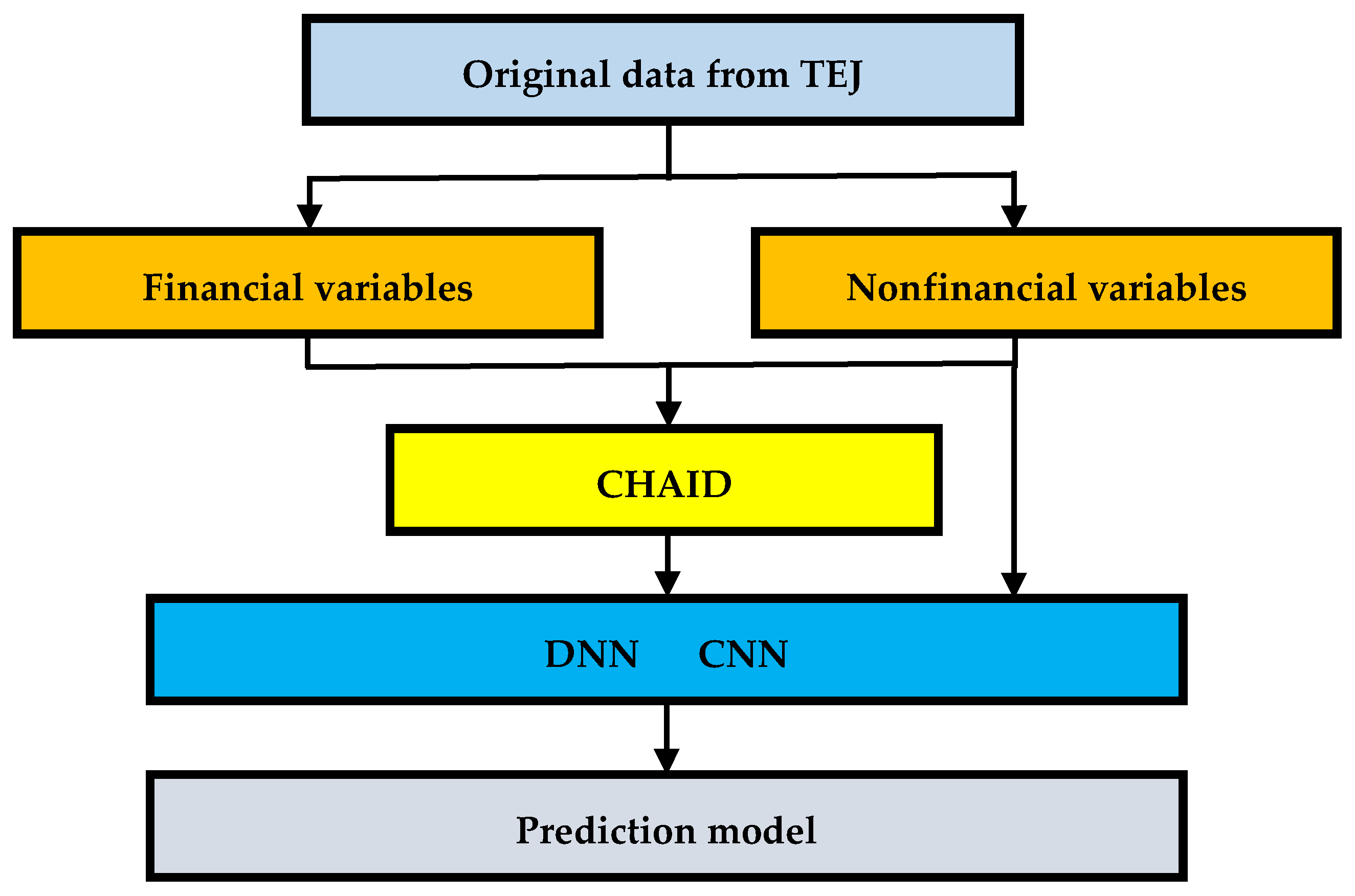
A parallel mode is designed for the research process in this study. On one hand, important variables are first selected by CHAID, then input them into DNN and CNN, respectively, for deep learning and repeatedly trained to build the optimal model. On the other hand, 23 variables are directly input into DNN and CNN, respectively, for deep learning and repeatedly trained to build the optimal model. The research design and process is shown in Figure 5:
4. Results
According to Section 3.6. Research Design and Process, a parallel mode is adopted in this study. On one hand, important variables are selected by CHAID in advance, then input into DNN and CNN, respectively, for deep learning and repeatedly trained to build the optimal model. On the other hand, 23 variables are directly input into DNN and CNN, respectively, for deep learning and repeatedly trained to build the optimal model. For the algorithms and coding of this study, please see the Supplementary Material. The important variables selected by CHAID as follows.
4.1. Important Variables Selected by CHAID
The IBM SPSS Modeler is utilized to conduct CHAID in this study. Nine important variables are first selected by CHAID, as shown in Table 3, including eight financial variables and one non-financial variable. In the order of their importance, X03: Debt ratio (VI = 0.5255), X16: EPS (VI = 0.0997), X23: Audited by BIG4 (VI = 0.0607), X18: Operating income ratio (VI = 0.0512), X19: Cash flow ratio (VI = 0.0488), X08: Times interest earned (VI = 0.0337), X04: D/E ratio (VI = 0.0318), X05: Ratio of long-term liabilities and shareholders’ equity (VI = 0.0284), X17: Gross margin (VI = 0.0276). Then, the nine important variables are input into DNN and CNN, respectively, for deep learning and repeatedly trained to build the optimal model.
4.2. Validation
In the process of modeling by DNN and CNN, this study refers to several deep learning papers [9,43,44]. 70% of all data is used for modeling, and 30% of all data is used for testing by random sampling without replacement in this study. 59.5% (85% × 70%) of all data is random sampling as the training dataset, which is used to fit the parameters of the model during the learning process, and is continuously optimized to obtain the best prediction model. 10.5% (15% × 70%) of all data is random sampling as the validation dataset to validate the state and convergence of models in the modeling process, in order to adjust the hyper-parameters and avoid over fitting. Finally, the remaining 30% of all data is used as the test dataset to assess the generalization and classification abilities of the model.
For deep learning algorithms, the value of all data has to be limited to between 0 and 1, so this study deletes the incomplete data in advance and normalizes the original data in the interval of 0 and 1.
This study uses accuracy, precision, sensitivity (recall), specificity, and F1 score as the performance indicators by the confusion matrix. In the process of modeling, a loss function is used to optimize the models, the lower the loss function value, and the higher accuracy of the model.
The Adam is utilized in the process of modeling to adjust the optimal parameters, which is in-sided of the TensorFlow (Keras. Optimizers. Adam). The optimal parameters of this study are: Learning rate = 0.001, beta 1 = 0.9, beta 2 = 0.999, epsilon = 1 × 10⁻⁷, batch size = 4, epochs = 150, dropout = 0.25, activation = ReLU and Sigmoid.
4.3. CHAID-DNN Model
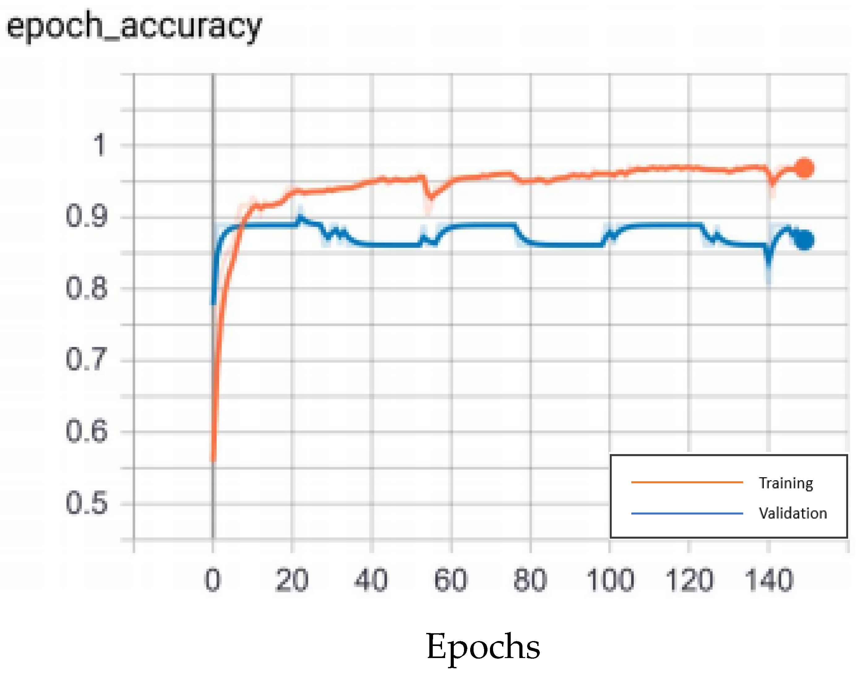
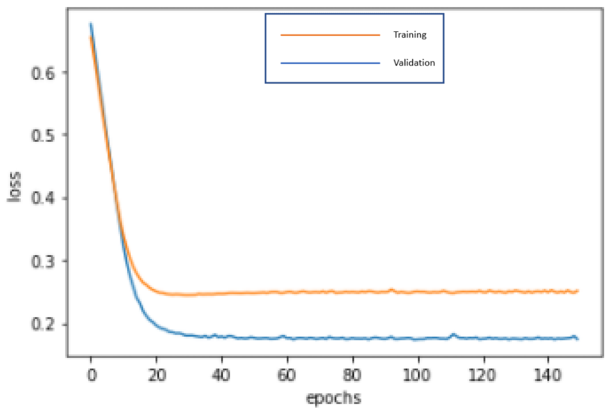
The nine important variables selected by CHAID are input into DNN for deep learning and repeatedly trained until reaching the optimal stable state, 150 epochs and 750 microseconds training time, in order to build the best model. The accuracy rates of the training dataset and validation dataset are 96.57% and 97.22%, respectively. In addition, the test dataset is used to test the prediction effect of the model, and an accuracy of 90.38% is obtained, including the type I error rate of 3.85% and the type II error rate of 5.77%. In the confusion matrix, the indicators of CHAID-DNN are: Accuracy = 90.38%, precision = 83.33%, sensitivity (recall) = 76.92%, specificity = 94.87%, F1-score = 80.00%. By these indicators, the performance of the model is good. In the process of modeling, the loss function with binary cross-entropy method is shown in Figure 6. Accuracy graph in the CHAID-DNN modeling process is shown in Figure 7.
4.4. CHAID-CNN Model
The nine important variables, as selected by CHAID are input into CNN for deep learning and repeatedly trained until reaching the optimal stable state, 150 epochs and 750 microseconds training time, in order to build the best model. The input data of this study is financial variables and non-financial variables, and a one-dimensional CNN is used in the modeling process. The input shape = (1, 9), batch size = 4, seq length = 1, filters = 16, stride = 1, padding = same, kernel size = 1, and pool size = 1 for the CHAID-CNN modeling in this study. The order of variables put into the CNN layer is: X03: Debt ratio, X04: D/E ratio, X05: Ratio of long-term liabilities and shareholders’ equity, X08: Times interest earned, X16: EPS, X17: Gross margin, X18: Operating income ratio, X19: Cash flow ratio, and X23: Audited by BIG4. The accuracy rates of the training dataset and validation dataset are 97.06% and 94.44%, respectively. In addition, the test dataset is used to test the prediction effect of the model, and an accuracy of 94.23% is obtained, including the type I error rate of 0.96% and the type II error rate of 4.81%. In the confusion matrix, the indicators of CHAID-CNN are: Accuracy = 94.23%, precision = 95.45%, sensitivity (recall) = 80.77%, specificity = 98.72%, F1-score = 87.50%. By these indicators, the performance of the model is pretty good. In the process of modeling, the loss function with binary cross-entropy method is shown in Figure 8. Accuracy graph in the CHAID-CNN modeling process is shown in Figure 9.
4.5. DNN Model
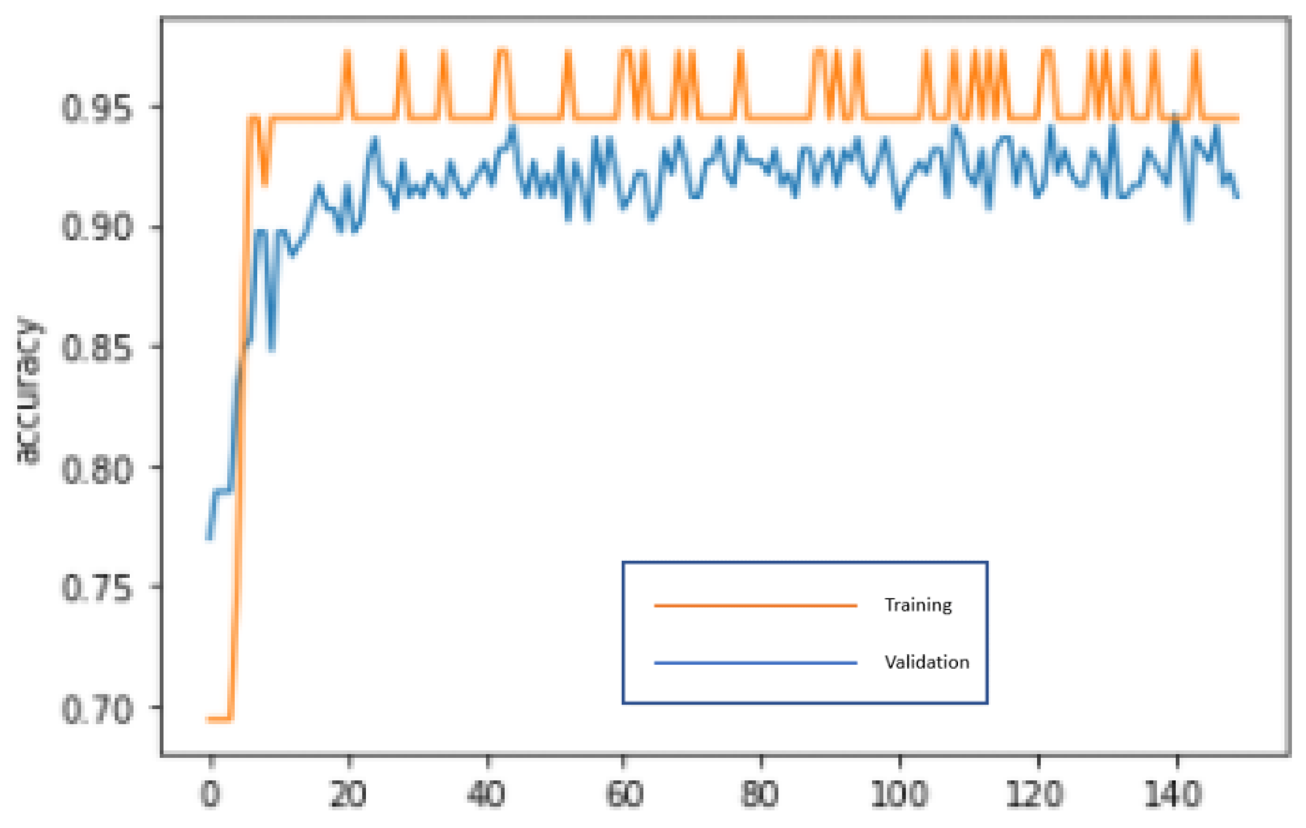
Without selecting the important variables by CHAID, 23 variables are input into DNN for deep learning and repeatedly trained until reaching the optimal stable state, 150 epochs and 750 microseconds training time, in order to build the best model. The accuracy rates of the training dataset and validation dataset are 91.67% and 94.44%, respectively. In addition, the test dataset is used to test the prediction effect of the model, and an accuracy of 89.42% is obtained, including the type I error rate of 5.77% and the type II error rate of 4.81%. In the confusion matrix, the indicators of DNN are: Accuracy = 89.42%, precision = 79.31%, sensitivity (recall) = 82.14%, specificity = 92.11%, F1-score = 80.70%. By these indicators, the performance of the model is good. In the process of modeling, the loss function with binary cross-entropy method is shown in Figure 10. Accuracy graph in the DNN modeling process is shown in Figure 11.
4.6. CNN Model
Without selecting the important variables by CHAID, 23 variables are input into CNN for deep learning and repeatedly trained until reaching the optimal stable state, 150 epochs and 750 microseconds training time, in order to build the best model. The input data of this study is financial variables and non-financial variables, and a one-dimensional CNN is used in the modeling process. The input shape = (1, 23), batch size = 4, seq length = 1, filters = 16, stride = 1, padding = same, kernel size = 1, and pool size = 1 for the CNN modeling in this study. The order of variables put into the CNN layer is: X03: Debt ratio, X04: D/E ratio, X05: Ratio of long-term liabilities and shareholders’ equity, X08: Times interest earned, X16: EPS, X17: Gross margin, X18: Operating income ratio, X19: Cash flow ratio, and X23: Audited by BIG4. The accuracy rates of the training dataset and validation dataset are 97.06% and 86.11%, respectively. In addition, the test dataset is used to test the prediction effect of the model, and an accuracy of 95.24% is obtained, including the type I error rate of 5.77% and the type II error rate of 1.92%. In the confusion matrix, the indicators of CNN are: Accuracy = 92.31%, precision = 81.82%, sensitivity (recall) = 93.10%, specificity = 92.00%, F1-score = 87.10%. By these indicators, the performance of the model is good. In the process of modeling, the loss function with binary cross-entropy method is shown in Figure 12. Accuracy graph in the CNN modeling process is shown in Figure 13.
4.7. Additional Comparison Models
In order to determine the usefulness of CHAID and make this study more complete, several comparison models are performed and discussed as follows:
4.7.1. CHAID-DNN Model Only with One Variable—Debt Ratio
As mentioned in Section 4.1, the “Debt ratio” is the most important variable (and extremely important; VI = 0.5255) that CHAID has screened out. The most important variable “Debt ratio” is input into DNN for deep learning and repeatedly trained until reaching the optimal stable state, 150 epochs and 500 microseconds training time, in order to build the best model. The accuracy rate of the test dataset is 89.42%. Although the accuracy rate is as high as 89.42%, it is not enough to use only one variable in practical applications. In the process of modeling, the loss function with binary cross-entropy method is shown in Figure 14. Accuracy graph in the CHAID-DNN modeling process (only with Debt ratio) is shown in Figure 15.
4.7.2. CHAID-CNN Model Only with One Variable—Debt Ratio
The most important variable “Debt ratio” selected by CHAID is input into CNN for deep learning and repeatedly trained until reaching the optimal stable state, 150 epochs and 750 microseconds training time, in order to build the best model. The accuracy rate of the test dataset is 92.31%. Although the accuracy rate is as high as 92.31%, it is not enough to use only one variable in practical applications. In the process of modeling, the loss function with binary cross-entropy method is shown in Figure 16. Accuracy graph in the CHAID-CNN modeling process (only with Debt ratio) is shown in Figure 17.
4.7.3. CHAID Model Only with One Variable—Debt Ratio
The most important variable “Debt ratio” is selected and modeling by CHAID. The accuracy rate of the test dataset is 90.74%. Although the accuracy rate is as high as 90.74%, it is not enough to use only one variable in practical applications. The CHAID modeling process (only with Debt ratio) is shown in Figure 18.
4.7.4. CHAID Model with Nine Important Variables
The nine important variables selected and modeling by CHAID. The accuracy rate of the test dataset is 91.67%. The CHAID modeling process (with nine variables) is shown in Figure 19.
5. Discussions
According to the traditional statistical view, especially regression analysis, it is necessary to select important variables before making predictions. However, as the two representative deep learning algorithms, DNN and RNN are very capable in learning, optimization, and prediction. Hence, the parallel mode is adopted in this study. On one hand, important variables are first selected by CHAID, then input them into DNN and CNN, respectively, for deep learning and repeatedly trained to build the optimal model. On the other hand, 23 variables are directly input into the DNN and CNN, respectively, for deep learning and repeatedly trained to build the optimal model. In the process of modeling by DNN and CNN, 70% of all data is used for modeling, and 30% of all data is used for testing by random sampling without replacement. 59.5% (85% × 70%) of all data is random sampling as the training dataset, which is used to fit the parameters of the model during the learning process, and is continuously optimized to obtain the best prediction model. 10.5% (15% × 70%) of all data is random sampling as the validation dataset to validate the state and convergence of models in the modeling process, in order to adjust the hyper-parameters and avoid over fitting. Finally, the remaining 30% of the all data is used as the test dataset to assess the generalization and classification abilities of the model.
Comparison of the performance of the four financial distress prediction models built in this study as shown in Table 4: The CHAID-CNN model has the highest accuracy (the accuracy of the test dataset is 94.23%, the type I error rate is 0.96%, and the type II error rate is 4.81%), followed by the CNN model (the accuracy of the test dataset is 92.31%; the type I error rate is 5.77%, the type II error rate is 1.92%), the CHAID-DNN model (the accuracy of the test dataset is 90.38%; the type I error rate is 3.85%, the type II error rate is 5.77%), and the DNN model (the accuracy of the test dataset is 89.42%; the type I error rate is 5.77%, the type II error rate is 4.81%). Although CNN is just one particular case of DNN, its more complex feedforward neural network can filter key variables from the data during the training process and focus on learning. CNN can process pictures, images, voices, and numbers more accurately. In general, CNN has a higher prediction accuracy rate than the DNN, and this is also supported by the results of this study.
According to the empirical results by the accuracy of test dataset: (1) The four financial distress prediction models built in this study all have very high accuracy, which is above 89%; (2) CNN has a higher prediction accuracy than DNN; (3) important variables are first selected by CHAID, and then, input into DNN and CNN to build the models, which are more accurate than the 23 variables directly input into DNN and CNN to build models without selection; (4) for the four financial distress prediction models, the type I error rates are all below 6%, and the type II error rates are also below 6%, indicating that the four models are all effective.
This study uses accuracy, precision, sensitivity (recall), specificity, and F1 score as the performance indicators by the confusion matrix, as shown in Table 5. By these indicators, all models reach the high level standard, and the CHAID-CNN model has the best performance.
Additional comparison models to determine the usefulness of CHAID are performed and discussed in Section 4.7. The usefulness of CHAID can be proven through these experiments.
In addition, in order to determine whether a company is in financial distress, the following important indices shall be considered: Nine important variables are selected by the CHAID in this study, including X03: Debt ratio (VI = 0.5255), X16: EPS (VI = 0.0997), X23: Audited by BIG4 (VI = 0.0607), X18: Operating income ratio (VI = 0.0512), X19: Cash flow ratio (VI = 0.0488), X08: Times interest earned (VI = 0.0337), X04: D/E ratio (VI = 0.0318), X05: Ratio of long-term liabilities and shareholders’ equity (VI = 0.0284), X17: Gross margin (VI = 0.0276). According to analysis, the comparison between the important indices and industry averages, or those of major competitors, shows that the debt ratio is higher; EPS is lower, and not audited by the BIG4 (the big four CPA firms); operating income ratio is lower; cash flow ratio is lower; interest coverage ratio is lower, and D/E ratio is higher; all the above factors are important indications of financial distress and deserve attention.
6. Conclusions and Suggestions
Because of the financial information asymmetry—financial condition and information are not transparent enough, the stakeholders usually do not know a company’s real financial condition until financial distress occurs. The company’s executives hold very different information from others. It is difficult for shareholders, creditors, employees, and other stakeholders to know the true face of the company’s financial condition. It often waits until the company experiences financial distress or bankruptcy.
The Enron case in the United States in 2001 made government agencies, scholars, industry, and the public face the importance of corporate governance and financial distress prevention. The Enron case was not only the largest bankruptcy in American history, it was also the largest audit failure. Due to the low corporate governance efficiency of a company, information will be non-transparent, meaning that outsiders cannot understand the companies’ actual financial conditions. As outsiders fail to know that companies are already in financial distress, it results in no warning being issued. Corporate financial distress prediction is very important for shareholders, investors, employees, creditors, and regulatory authorities.
Generally, due to information asymmetry, investors often do not know that a company may be in financial distress until its official financial statement is issued. If company executives deliberately glamorize or falsify financial statements to conceal the actual operating or financial conditions of companies, investors will have less opportunities to obtain true financial information. As financial distress prediction reveals potential financial deficiencies or risks, it can improve investors’ decision-making, assist financial institutions in their lending decisions, and help regulatory authorities to formulate regulations. Hence, effective financial distress prediction models have become crucial for assessments of continuous financial feasibility. Corporate financial distress often occurs, and causes great losses to stakeholders; therefore, financial distress prediction is of great significance to corporate sustainable development.
In the era of artificial intelligence (AI), deep learning algorithms are used in academic research. So far, quite a few studies have used deep learning algorithms to predict financial distress. This study tries to offer a more innovative approach in financial distress study, and it can make some direct contributions to academic research and the practice of financial distress prediction. The purpose of this study is to construct highly-accurate and effective financial distress prediction models through two representative deep learning algorithms: Deep neural networks (DNN) and convolutional neural networks (CNN). In addition, important variables are selected by the chi-squared automatic interaction detector (CHAID). Of the four financial distress prediction models built in this study, CHAID-CNN has the highest accuracy (the accuracy of the test dataset is 94.23%, the type I error rate is 0.96%, and the type II error rate is 4.81%), followed by CNN (the accuracy of the test dataset is 92.31%; the type I error rate is 5.77%, the type II error rate is 1.92%), CHAID-DNN (the accuracy of the test dataset is 90.38%; the type I error rate is 3.85%, the type II error rate is 5.77%), and DNN (the accuracy of the test dataset is 89.42%; the type I error rate is 5.77%, the type II error rate is 4.81%).
According to the empirical results: (1) For the social science research, the four financial distress prediction models built in this study all have very high accuracy rates, which are above 89%; (2) CNN has a higher prediction accuracy rate than DNN; (3) important variables are first selected by CHAID, and then, input into DNN and CNN to build the models, which are more accurate than the 23 variables directly input into DNN and CNN to build models without selection; (4) for the four financial distress prediction models, the type I error rates are all below 6% and the type II error rates are also below 6%, indicating that they are effective.
In order to protect the interests of stakeholders, this study suggests that:
(1.) Government authorities shall strictly monitor corporate financial conditions and enact strict regulations on corporate financial supervision and corporate governance.
(2.) Banks shall strengthen both credit investigations and loan granting, and pay attention to corporate reputation and revenue, as well as the credit status of corporate owners, in order to conduct financial transactions and financing for companies.
(3.) CPAs and auditors must fully comply with auditing regulations and their professional norms, require that companies provide correct and complete financial information, and verify relevant qualifications when reviewing corporate financial statements.
(4.) Companies’ independent directors and supervisors shall fulfill their responsibilities to check on financial conditions for shareholders.
(5.) Companies shall strengthen their internal control systems to prevent financial distress, which can avoid malpractices, concealment, frauds, and the inside activities of managers and employees, in addition to effectively controlling corporate financial risks.
Finally, this study aims at the rigor of design and demonstration regarding the samples and data from Taiwan’s listed and OTC companies. However, due to different economic and financial environments, as well as the financial regulations of different countries, regions, or economies, the results of this study cannot be applied to all situations, which is the inevitable limitation of relevant studies.
Supplementary Materials
Please see https://www.mdpi.com/2073-8994/13/3/443/s1.
Funding
This research received no external funding.
Institutional Review Board Statement
Not applicable.
Informed Consent Statement
Not applicable.
Data Availability Statement
The data of this study is taken from the Taiwan Economic Journal (TEJ) Database. This is a paid database and not free. Thanks! The data of this study is available online: https://drive.google.com/drive/folders/1grjQFgkWL8Pma60N9iXKQVVy2wZOi8s5?usp=sharing (accessed on 8 March 2021).
Acknowledgments
The author would like to thank the editors and the anonymous reviewers of this journal.
Conflicts of Interest
The author declares no conflict of interest.
References
- Chen, S.; Shen, Z.-D. Financial Distress Prediction Using Hybrid Machine Learning Techniques. Asian J. Econ. Bus. Account. 2020, 16, 1–12. [Google Scholar] [CrossRef]
- Woodlock, P.; Dangol, R. Managing Bankruptcy and Default Risk. J. Corp. Account. Financ. 2014, 26, 33–38. [Google Scholar] [CrossRef]
- Evans, J.; Borders, A.L. Strategically Surviving Bankruptcy during a Global Financial Crisis: The Importance of Understanding Chapter 15. J. Bus. Res. 2014, 67, 2738–2742. [Google Scholar] [CrossRef]
- Jensen, M.C.; Meckling, W.H. Theory of the Firm: Managerial Behavior, Agency Costs and Ownership Structure. SSRN Electron. J. 1998, 163–231. [Google Scholar] [CrossRef]
- Inekwe, J.N.; Jin, Y.; Valenzuela, M.R. The effects of financial distress: Evidence from US GDP growth. Econ. Model. 2018, 72, 8–21. [Google Scholar] [CrossRef]
- Wu, L.; Shao, Z.; Yang, C.; Ding, T.; Zhang, W. The Impact of CSR and Financial Distress on Financial Performance—Evidence from Chinese Listed Companies of the Manufacturing Industry. Sustainability 2020, 12, 6799. [Google Scholar] [CrossRef]
- Jandik, T.; Makhija, A.K. Debt, debt structure and corporate performance after unsuccessful takeovers: Evidence from targets that remain independent. J. Corp. Financ. 2005, 11, 882–914. [Google Scholar] [CrossRef]
- Chen, W.-S.; Du, Y.-K. Using neural networks and data mining techniques for the financial distress prediction model. Expert Syst. Appl. 2009, 36, 4075–4086. [Google Scholar] [CrossRef]
- Gregova, E.; Valaskova, K.; Adamko, P.; Tumpach, M.; Jaros, J. Predicting Financial Distress of Slovak Enterprises: Comparison of Selected Traditional and Learning Algorithms Methods. Sustainability 2020, 12, 3954. [Google Scholar] [CrossRef]
- Chen, S.D.; Jhuang, S. Financial distress prediction using data mining techniques. ICIC-ELB 2018, 9, 131–136. [Google Scholar]
- Hahnenstein, L.; Köchling, G.; Posch, P.N. Do firms hedge in order to avoid financial distress costs? New empirical evidence using bank data. J. Bus. Financ. Account. 2020, 1–24. [Google Scholar] [CrossRef]
- Sharma, S.; Mahajan, V. Early Warning Indicators of Business Failure. J. Mark. 1980, 44, 80. [Google Scholar] [CrossRef]
- Felipe, C.M.; Roldán, J.L.; Leal-Rodríguez, A.L. An explanatory and predictive model for organizational agility. J. Bus. Res. 2016, 69, 4624–4631. [Google Scholar] [CrossRef]
- Shen, F.; Liu, Y.; Wang, R.; Zhou, W. A dynamic financial distress forecast model with multiple forecast results under unbal-anced data environment. Knowl. Based. Syst. 2020, 192, 1–16. [Google Scholar] [CrossRef]
- Fama, E.; Jensen, M. Separation of ownership and control. J. Law Econ. 1983, 26, 301–325. [Google Scholar] [CrossRef]
- Dowell, G.W.S.; Shackell, M.B.; Stuart, N.V. Boards, CEOs, and surviving a financial crisis: Evidence from the internet shakeout. Strat. Manag. J. 2011, 32, 1025–1045. [Google Scholar] [CrossRef]
- Mangena, M.; Tauringana, V.; Chamisa, E. Corporate Boards, Ownership Structure and Firm Performance in an Environment of Severe Political and Economic Crisis. Br. J. Manag. 2011, 23, S23–S41. [Google Scholar] [CrossRef]
- Tinoco, M.H.; Wilson, N. Financial distress and bankruptcy prediction among listed companies using accounting, market and macroeconomic variables. Int. Rev. Financ. Anal. 2013, 30, 394–419. [Google Scholar] [CrossRef]
- Manzaneque, M.; Merino, E.; Priego, A.M. The role of institutional shareholders as owners and directors and the financial distress likelihood. Evidence from a concentrated ownership context. Eur. Manag. J. 2016, 34, 439–451. [Google Scholar] [CrossRef]
- Mangena, M.; Priego, A.M.; Manzaneque, M. Bank power, block ownership, boards and financial distress likelihood: An in-vestigation of Spanish listed firms. J. Corp. Financ. 2020, 64, 1–22. [Google Scholar] [CrossRef]
- Akerlof, G.A. The Market for “Lemons”: Quality Uncertainty and the Market Mechanism. Q. J. Econ. 1970, 84, 488–500. [Google Scholar] [CrossRef]
- Yan, D.; Chi, G.; Lai, K.K. Financial Distress Prediction and Feature Selection in Multiple Periods by Lassoing Unconstrained Distributed Lag Non-linear Models. Mathematics 2020, 8, 1275. [Google Scholar] [CrossRef]
- Beaver, W. Financial ratios as predictors of failure, empirical research in accounting: Selected studied. J. Account. Res. 1966, 4, 71–111. [Google Scholar] [CrossRef]
- Altman, E.I. Financial ratios, discriminant analysis and the prediction of corporate bankruptcy. J. Financ. 1968, 23, 589–609. [Google Scholar] [CrossRef]
- Altman, E.I.; Iwanicz-Drozdowska, M.; Laitinen, E.K.; Suvas, A. Financial Distress Prediction in an International Context: A Review and Empirical Analysis of Altman’s Z-Score Model. J. Int. Financ. Manag. Account. 2017, 28, 131–171. [Google Scholar] [CrossRef]
- Blum, M. Failing Company Discriminant Analysis. J. Account. Res. 1974, 12, 1–25. [Google Scholar] [CrossRef]
- Altman, E.I.; Haldeman, R.G.; Narayanan, P. ZETATM analysis A new model to identify bankruptcy risk of corporations. J. Bank. Financ. 1977, 1, 29–54. [Google Scholar] [CrossRef]
- Ohlson, J.A. financial ratios and the probability prediction of bankruptcy. J. Account. Res. 1980, 18, 109–131. [Google Scholar] [CrossRef] [Green Version]
- Dimitras, A.I.; Zanakis, S.H.; Zopounidis, C. A survey of business failure with an emphasis on prediction methods and indus-trial applications. Eur. J. Oper. Res. 1966, 90, 487–513. [Google Scholar] [CrossRef]
- Jones, S.; Hensher, D.A. Predicting Firm Financial Distress: A Mixed Logit Model. Account. Rev. 2004, 79, 1011–1038. [Google Scholar] [CrossRef]
- Tinoco, M.H.; Holmes, P.; Wilson, N. Polytomous response financial distress models: The role of accounting, market and macroeconomic variables. Int. Rev. Financ. Anal. 2018, 59, 276–289. [Google Scholar] [CrossRef] [Green Version]
- Yao, S. “Who Should Be the Next CEO?” Desirable Successor Characteristics in Recovery from Financial Distress. Emerg. Mark. Financ. Trade 2020, 1–12. [Google Scholar] [CrossRef]
- Yeh, C.C.; Chi, D.J.; Hsu, M.F. A hybrid approach of DEA, rough set and support vector machines for business failure predic-tion. Expert Syst. Appl. 2010, 37, 1535–1541. [Google Scholar] [CrossRef]
- Chen, M.-Y. Predicting corporate financial distress based on integration of decision tree classification and logistic regression. Expert Syst. Appl. 2011, 38, 11261–11272. [Google Scholar] [CrossRef]
- Hsieh, T.-J.; Hsiao, H.-F.; Yeh, W.-C. Mining financial distress trend data using penalty guided support vector machines based on hybrid of particle swarm optimization and artificial bee colony algorithm. Neurocomputing 2012, 82, 196–206. [Google Scholar] [CrossRef]
- Kim, S.Y.; Upneja, A. Predicting restaurant financial distress using decision tree and AdaBoosted decision tree models. Econ. Model. 2014, 36, 354–362. [Google Scholar] [CrossRef]
- Geng, R.; Bose, I.; Chen, X. Prediction of financial distress: An empirical study of listed Chinese companies using data mining. Eur. J. Oper. Res. 2015, 241, 236–247. [Google Scholar] [CrossRef]
- Jan, C.L.; Haiso, D. Detection of fraudulent financial statements using decision tree and artificial neural network. ICIC-ELB 2018, 9, 347–352. [Google Scholar]
- Huang, Y.P.; Yen, M.F. A new perspective of performance comparison among machine learning algorithms for financial distress prediction. Appl. Soft Comput. 2019, 83, 105663–105677. [Google Scholar] [CrossRef]
- Sun, J.; Li, H.; Fujita, H.; Fu, B.; Ai, W. Class-imbalanced dynamic financial distress prediction based on Adaboost-SVM en-semble combined with SMOTE and time weighting. Inf. Fusion. 2020, 54, 128–144. [Google Scholar] [CrossRef]
- Kass, G.V. Significance Testing in Automatic Interaction Detection (A.I.D.). J. R. Stat. Soc. Ser. C Appl. Stat. 1975, 24, 178. [Google Scholar] [CrossRef]
- Jan, C.-L. An Effective Financial Statements Fraud Detection Model for the Sustainable Development of Financial Markets: Evidence from Taiwan. Sustainability 2018, 10, 513. [Google Scholar] [CrossRef] [Green Version]
- Dencker, T.; Klinkisch, P.; Maul, S.M.; Ommer, B. Deep learning of cuneiform sign detection with weak supervision using transliteration alignment. PLoS ONE 2020, 15, e0243039. [Google Scholar] [CrossRef] [PubMed]
- Matsuzaka, Y.; Uesawa, Y. A Molecular Image-Based Novel Quantitative Structure-Activity Relationship Approach, Deepsnap-Deep Learning and Machine Learning. Curr. Issues Mol. Biol. 2020, 42, 455–472. [Google Scholar] [CrossRef] [PubMed]
Figure 1.
CHAID (chi-squared automatic interaction detector) classification structure.

Figure 2.
DNN (deep neural network) structure.

Figure 3.
Hidden layer calculation.

Figure 4.
The convolutional neural networks (CNN) process of this study.

Figure 5.
Research design and process.

Figure 6.
Loss function graph of CHAID-DNN modeling.

Figure 7.
Accuracy graph in the CHAID-DNN modeling process.

Figure 8.
Loss function graph of CHAID-CNN modeling.

Figure 9.
Accuracy graph in the CHAID-CNN modeling process.

Figure 10.
Loss function graph of DNN modeling.

Figure 11.
Accuracy graph in the DNN modeling process.

Figure 12.
Loss function graph of CNN modeling.

Figure 13.
Accuracy graph in the CNN modeling process.

Figure 14.
Loss function graph of CHAID-DNN modeling only with Debt ratio.

Figure 15.
Accuracy graph in the CHAID-DNN modeling process only with Debt ratio.

Figure 16.
Loss function graph of CHAID-CNN modeling only with debt ratio.

Figure 17.
Accuracy graph in the CHAID-CNN modeling process only with debt ratio.

Figure 18.
The CHAID modeling process only with debt ratio.

Figure 19.
The CHAID modeling process with nine variables.


Table 1.
Sample distribution.
| Industry Classification | Number of Companies in Financial Distress | Number of Companies not in Financial Distress |
|---|---|---|
| Semiconductors | 4 | 12 |
| Optoelectronics | 6 | 18 |
| Electric machinery | 3 | 9 |
| Communication networks | 2 | 6 |
| Electronic parts and components | 10 | 30 |
| Other electronic industries | 2 | 6 |
| Electronic commerce | 1 | 3 |
| Information service industry | 2 | 6 |
| Computers and peripheral equipment | 3 | 9 |
| Chemical industry | 1 | 3 |
| Biotechnology and medical treatment | 3 | 9 |
| Steel industry | 7 | 21 |
| Building materials manufacturing | 16 | 48 |
| Cement industry | 1 | 3 |
| Oil, electricity and gas industry | 1 | 3 |
| Shipping industry | 1 | 3 |
| Rubber industry | 1 | 3 |
| Plastics industry | 1 | 3 |
| Textile fiber | 4 | 12 |
| Food industry | 1 | 3 |
| Cultural and creative industries | 2 | 6 |
| Trade and merchandise industry | 2 | 6 |
| Others | 10 | 30 |
| Total | 86 | 258 |
Table 2.
Research variables.
| No. | Variable | Description |
|---|---|---|
| X01 | Current ratio | Current assets/current liabilities |
| X02 | Quick ratio | Quick assets/current liabilities |
| X03 | Debt ratio | Total liabilities/total assets |
| X04 | D/E ratio | Total liabilities/total equity |
| X05 | Ratio of long-term liabilities and shareholders’ equity | Long-term liabilities/total equity |
| X06 | Current liabilities ratio | Current liabilities/total liabilities |
| X07 | Long-term liabilities ratio | Long-term liabilities/total liabilities |
| X08 | Times interest earned | EBIT/interest expense |
| X09 | Ratio of long-term funds to fixed assets | (Shareholders’ equity + long-term liabilities)/fixed assets |
| X10 | Ratio of fixed assets to long-term liabilities | Fixed assets/long-term liabilities |
| X11 | ROE | Net income/average total equity |
| X12 | ROA | (Net income + interest expense × (1-tax rate))/average total assets |
| X13 | Accounts receivable turnover | Net sales/average accounts receivable |
| X14 | Inventory turnover | Cost of goods sold/average inventory |
| X15 | Total fixed assets turnover | Net sales/total fixed assets |
| X16 | EPS | Net income/shares of common stock |
| X17 | Gross margin | Gross profit/net sales |
| X18 | Operating income ratio | Operating income/net sales |
| X19 | Cash flow ratio | Operating cash flow/current liabilities |
| X20 | Pledge ratio of directors and supervisors | Number of pledged shares of directors and supervisors/number of shares held by directors and supervisors |
| X21 | Stockholding ratio of directors and supervisors | Number of shares held by directors and supervisors/shares of common stock |
| X22 | Stockholding ratio of majority shareholders | Number of shares held by majority shareholders/shares of common stock |
| X23 | Audited by BIG4 (the big four CPA firms) or not | 1 for companies audited by BIG4, otherwise 0 |
Table 3.
Important variables selected by CHAID.
| No. | Variable | Variable Importance |
|---|---|---|
| X03 | Debt ratio | 0.5255 |
| X16 | EPS | 0.0997 |
| X23 | Audited by BIG4 | 0.0607 |
| X18 | Operating income ratio | 0.0512 |
| X19 | Cash flow ratio | 0.0488 |
| X08 | Times interest earned | 0.0337 |
| X04 | D/E ratio | 0.0318 |
| X05 | Ratio of long-term liabilities and shareholders’ equity | 0.0284 |
| X17 | Gross margin | 0.0276 |
Table 4.
Summary of accuracy of all models.
| Model | Training Dataset | Validation Dataset | Test Dataset | Average | Type I Error | Type II Error |
|---|---|---|---|---|---|---|
| CHAID-DNN | 96.57% | 97.22% | 90.38% | 94.72% | 3.85% | 5.77% |
| CHAID-CNN | 97.06% | 94.44% | 94.23% | 95.24% | 0.96% | 4.81% |
| DNN | 91.67% | 94.44% | 89.42% | 91.84% | 5.77% | 4.81% |
| CNN | 97.06% | 86.11% | 92.31% | 95.24% | 5.77% | 1.92% |
Table 5.
Confusion matrix indicators.
| Model | Accuracy | Precision | Sensitivity (Recall) | Specificity | F1 Score | Training Time |
|---|---|---|---|---|---|---|
| CHAID-DNN | 90.38% | 83.33% | 76.92% | 94.87% | 80.00% | 750 us |
| CHAID-CNN | 94.23% | 95.45% | 80.77% | 98.72% | 87.50% | 750 us |
| DNN | 89.42% | 79.31% | 82.14% | 92.11% | 80.70% | 750 us |
| CNN | 92.31% | 81.82% | 93.10% | 92.00% | 87.10% | 750 us |
Publisher’s Note: MDPI stays neutral with regard to jurisdictional claims in published maps and institutional affiliations. |
© 2021 by the author. Licensee MDPI, Basel, Switzerland. This article is an open access article distributed under the terms and conditions of the Creative Commons Attribution (CC BY) license (http://creativecommons.org/licenses/by/4.0/).
Share and Cite
MDPI and ACS Style
Jan, C.-l. Financial Information Asymmetry: Using Deep Learning Algorithms to Predict Financial Distress. Symmetry 2021, 13, 443. https://doi.org/10.3390/sym13030443
AMA Style
Jan C-l. Financial Information Asymmetry: Using Deep Learning Algorithms to Predict Financial Distress. Symmetry. 2021; 13(3):443. https://doi.org/10.3390/sym13030443
Chicago/Turabian StyleJan, Chyan-long. 2021. "Financial Information Asymmetry: Using Deep Learning Algorithms to Predict Financial Distress" Symmetry 13, no. 3: 443. https://doi.org/10.3390/sym13030443
Note that from the first issue of 2016, this journal uses article numbers instead of page numbers. See further details here.