Article

A Kinetic Theory Model of the Dynamics of Liquidity Profiles on Interbank Networks

by
Marina Dolfin
1,2,*,†,
Leone Leonida
2,3,† and
Eleonora Muzzupappa
2,3,†
1
Department of Engineering, University of Messina, 98166 Messina, Italy
2
Business School, King’s College London, London WC2B 4BG, UK
3
Centro di Scienze Economiche Aziendali e Metodi Quantitativi (SEAM), University of Messina, 98166 Messina, Italy
*
Author to whom correspondence should be addressed.
These authors contributed equally to this work.
Symmetry 2021, 13(2), 363; https://doi.org/10.3390/sym13020363
Submission received: 26 January 2021 / Revised: 15 February 2021 / Accepted: 15 February 2021 / Published: 23 February 2021

Abstract

:
This paper adopts the Kinetic Theory for Active Particles (KTAP) approach to model the dynamics of liquidity profiles on a complex adaptive network system that mimic a stylized financial market. Individual incentives of investors to form or delete a link is driven, in our modelling framework, by stochastic game-type interactions modelling the phenomenology related to policy rules implemented under Basel III, and it is exogeneously and dynamically influenced by a measure of overnight interest rate. The strategic network formation dynamics that emerges from the introduced transition probabilities modelling individual incentives of investors to form or delete links, provides a wide range of measures using which networks might be considered “best” from the point of view of the overall welfare of the system. We use the time evolution of the aggregate degree of connectivity to measure the time evolving network efficiency in two different scenarios, suggesting a first analysis of the stability of the arising and evolving network structures.

1. Introduction

We introduce here the mathematical modelling framework adopted throughout the paper to model a dynamics of liquidity on a time evolving network that mimics a stylized financial market, following hints and research perspectives that arose in [1,2]. The kinetic theory of active particles (KTAP) provides in fact mathematical tools to transfer into a mathematical model the collective dynamics of large systems of interacting living entities, which perfectly fit the peculiar phenomenology of financial markets. The main features of the KTAP approach are the following:
  • The overall state of the system under consideration, a stylized financial market in the present paper, is described by a probability distribution over the micro-scale state of the active particles whose state includes, in addition to mechanical variables, a variable called activity, which describes the state of each individual entity. Hence, the said probability distribution is the dependent variable, while the activity is the micro-state. In the following we will specify what activity represents in our model, specifically referring to liquidity of assets.
  • Interactions are modeled by mathematical tools of stochastic game theory. The output depends on the micro-state of the interacting entities and on the strategy they adopt to reach their pay-off, which is heterogeneously distributed over the active particles. In general, interactions are nonlocal and nonlinearly additive and that is the case of our model.
  • The KTAP approach allows for transferring the interactions output into the dynamics, across time and space, of the dependent variable, accounting both for “rational” or even “irrational” strategies (see [1] for a detailed discussion on this point that is widely debated in the economic literature).
The class of systems under consideration are complex in such a way that the dynamic of the single entities does not lead straightforwardly to the dynamics of the whole system, due to peculiar nonlinear interactions. A symmetry analysis might be necessary in modeling the interactions, which might be not symmetric, as in many different applications discussed below. For a more detailed explanation of the mathematical theory, the reader may want to refer to the book [3] and to the survey [4], which are mainly focused on the modeling of social systems. The general framework is that of behavioral systems [5] and the complexity of living systems [6].
There exists a wide array of applications studied in the literature on that topic by using the tools of the KTAP theory. Some very recent ones can be mentioned without claim of completeness. Among the most recent studies we draw from—learning dynamics [7] or opinion dynamics related to diffusive dynamics [8], frontiers of equity risk [9], immune competition between cancer and immune cells [10], vehicular traffic [11], dynamics of human crowds [12,13,14,15] and motility of human cells [16]. Applications have generated challenging analytic problems, for instance symmetry analysis [17] or derivation of macroscopic equations from the underlying description at the micro-scale [18] (a short example is also provided here in the Appendix A). An example of a challenging computational problem can be found in [19].
Our paper adopts the tools within the KTAP approach to model the dynamics of liquidity profiles in a stylized model of an interbank network. It moves in quite the opposite direction with respect to that in [20], where the authors try to infer how banks manage their liquidity ratios based on the interbank network characteristics. We reverse, in fact, this point of view, by inquiring how liquidity ratios of a system of interconnected banks may shape the evolving network of their interconnections.
The actual approach with KTAP tools requires two steps. The first step involves the derivation of the general mathematical structure, which captures the main features of the system under consideration. The second step refers to the derivation of models, which is obtained by inserting into the above structure the specific interactions between active particles. Although this paper is mainly focused on using the KTAP approach, we mention that parallel methods have been proposed in the literature; as an example the mathematical theory of behavioral swarms [21,22] and methods of the kinetic theory and Fokker Plank equations [23].
The paper proceeds as follows—Section 2 provides a concise phenomenological description of the process under consideration, characterizing the dynamics of liquidity on a time evolving network; Section 3 provides a description of the class of dynamical systems under consideration and the derivation of the specific mathematical model that describes the phenomenology; Section 4 is devoted to simulations in two case studies and the related interpretations of outcomes; Section 5 looks ahead to research perspectives. A short appendix devoted to some analytical derivations of the necessary conditions for equilibrium configurations of high quality liquid assets on time evolving networks closes the paper.

2. Liquidity Profile of Financial Institutions and Regulation Policies for Banks

We will introduce in the following the liquid asset ratio that provides an indication of the liquidity available to meet expected and unexpected demands for cash. Its actual definition involves the level of liquidity that indicate the ability of the deposit-taking sector to withstand shocks to their balance sheet.

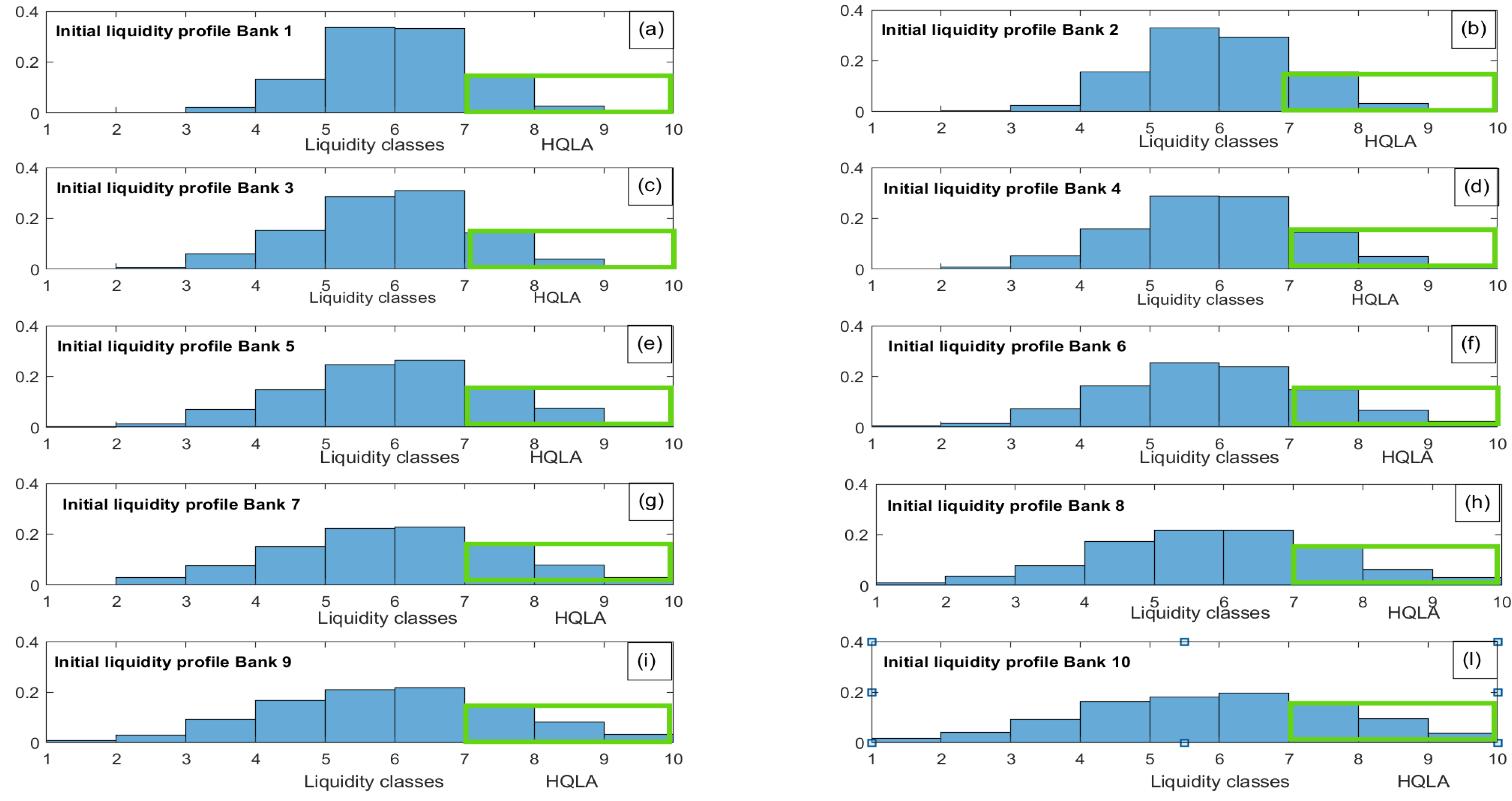
2.1. Banks’ Assets and Dynamics of Liquidity Profiles

The definition of liquid assets is based on the fundamental property of the assets to be quickly converted into cash if needed to meet financial obligations. Central bank reserves and government bonds are typical examples of liquid assets, and a safe policy should envisage to have enough liquid assets to meet possible withdrawals by depositors or any near-term obligation.
The inter-bank overnight rate on each day is defined by the opportunity cost of holding reserves on that day. Overnight rates are determined not only by the current condition, however, but also by the expectations on liquidity conditions for the maintenance period. If the market rate is low in relation to expected overnight rates over the given period, banks have an incentive to hold reserve surpluses, and the opposite instead whenever the market rate is high. This dynamics will tend to stabilise market rates, determining a tendency for the overnight rates to align with future expected overnight rates within the maintenance period.
The dynamics of liquidity in financial systems is a hot topic, due to the crucial role they played during the financial crisis. During the Global Financial Crisis (GFC) there has been provided by the U.S. government several trillions dollars to the financial sector to face a liquidity crisis and then impede the collapse of the whole system. The need for financial stability and portfolio management dynamics, call for higher attention to measuring and modelling liquidity dynamics.
In the aftermath of the GFC, the quest has been for a new prudential regulatory framework, able to cope with crisis phenomena. This explains the importance of resorting to mathematical modeling to test the performance of these new financial regulation, such as those implemented by the Basel III framework [24,25].
The impact that new policies and regulations may have on the financial sector poses new challenges and issues that require an interdisciplinary approach among scholars. The statistical techniques used to quantify and manage risk have improved over time. Basel III and economic liquidity risk are used, beyond the banking system, by software companies and consulting companies as a market target. The relevant literature in the field proposes quantitative measurement in order to cope with the complexity of the interactions as, for instance, the liquidity mismatch index (LMI) proposed in [26], even if there is still little consensus about how to measure liquidity and liquidity risk [27].
A relevant example may be the relationship between liquidity and prices (overnight inter-bank rates) in the inter-bank money market that is aimed at satisfying the liquidity needs of the banking systems. In fact, the European Central Bank (ECB) requires that banks of the Euro zone deposit reserves in the respective national central bank, in the proportion of (2%) of the total deposits and debts owned by the bank, considering a maintenance period of one month from the 24th of a month to the 23rd of the following. This regulatory constraint is inducing banks to exchange liquidity with each other in order to minimize the associated implicit costs, as well as satisfying the constraint [28]. Until 2000 they were executed at a fixed interest rate. Since then they have been conducted with a variable rate. However, the relationship between liquidity and prices may not be totally independent from the structure and efficiency on the relevant market. That is why the interbank lending, even if constituting a sort of mutual insurance by representing a safety net for banks, may be a source of systemic risk in some specific situations [28].
We study the dynamics in the liquidity profile of a financial system, arising when individuals interact through financial transaction on the market, by resorting to statistical methods for complex systems modelling the dynamics of the liquidity risk profile of a stylized financial system, artificially experimenting with liquidity management in the banking system.

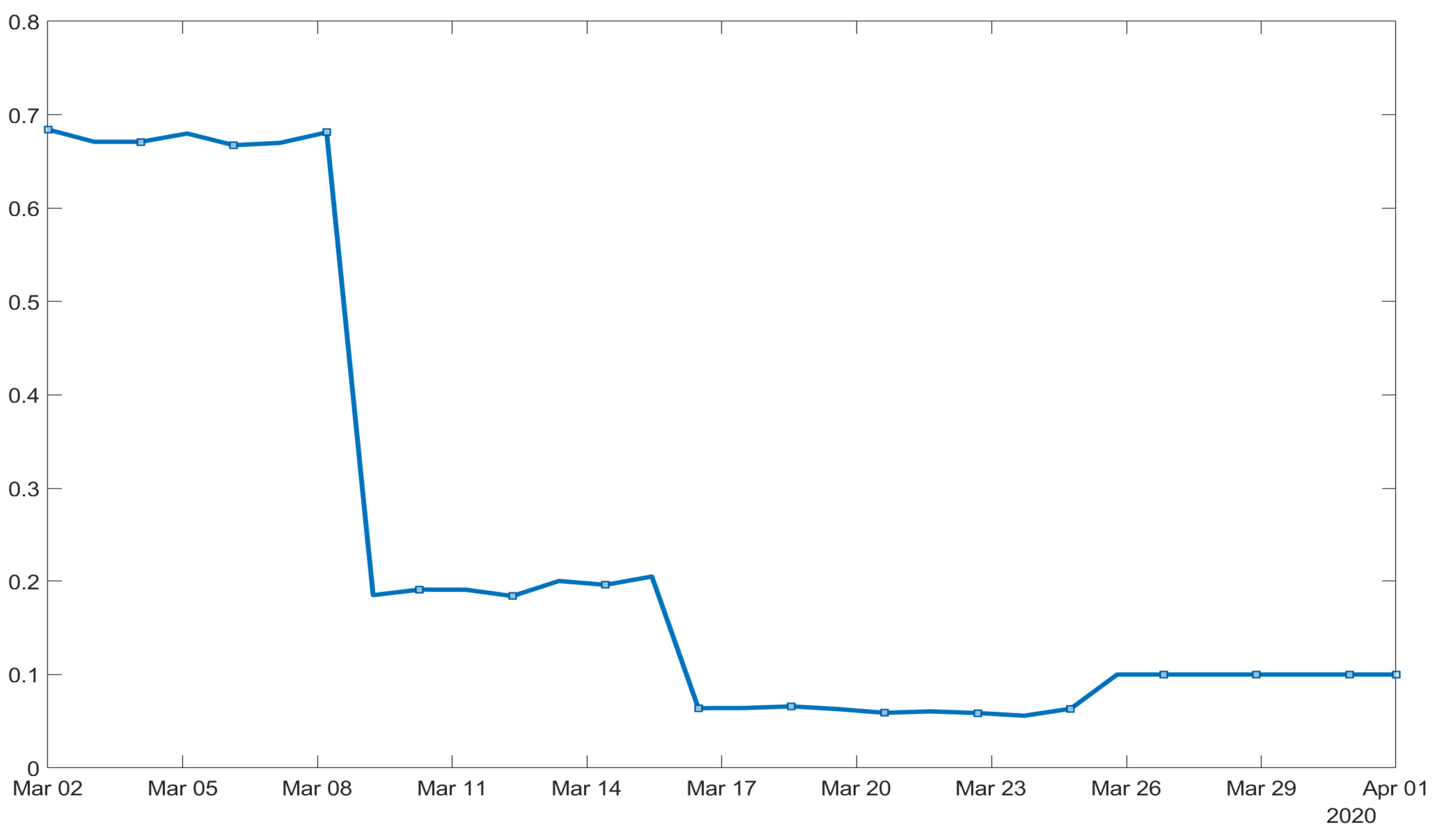
2.2. The Liquidity Coverage Ratio

The liquidity coverage ratio (LCR) quantifies the proportion of highly liquid assets held by a financial institution. It measures the capability of the institution to meet short-term obligations and it can be used as a generic stress test for capital preservation, preventing possible market-wide shocks. It is based on the percentage of high quality liquid assets (HQLA) in a financial institution’s portfolio, which consists of cash, or assets that can be easily converted into cash, at little or no loss of value (it can include cash, Treasury bonds and corporate debt). It comprises Level 1 and Level 2 (A and B) assets [24]. Specifically, under Basel III, Level 2 assets should account for no more than 40% of a bank’s HQLA, with Level 2B accounting for no more than 15%.
LCR is a stress measure for the liquidity needs for a 30 calendar days liquidity stress scenario and it is an important measure within the rules of Basel Accords, developed by the Basel Committee on Banking Supervision (BCBS). It has been introduced with the aim of fostering banks’ resilience in case of a financial crisis, by providing a cushion of cash sufficient at least for the minimum period of 30 days. It is obtained by dividing HQLA by the total net cash outflows, over a 30-day stress period. The total net cash outflows is given by the total expected cash outflows minus the total expected cash inflows, calculated in the specified stress scenario for the subsequent 30 calendar days (to specific definition to calculate expected cash outflows and inflows see Annex 1 of [24] providing a summary description of LCR).
The LCR was proposed in 2010 with revisions and final approval in 2014 [24]. The full 100% minimum was not required until 2019. LCR applies to all banking institutions that have more than $250 billion in total consolidated assets or more than $10 billion in on-balance sheet foreign exposure. Such banks, often referred to as “Systematically Important Financial Institutions (SIFI)”, are required to maintain a 100% LCR, which means holding an amount of highly liquid assets that are equal or greater than its net cash flow, over a 30-day stress period. On the balance sheet, assets become less liquid by their hierarchy. As such, the long-term assets portion of the balance sheet includes non-liquid assets. These assets are expected for cash conversion in one year or more. Land, real estate investments, equipment, and machinery are considered types of non-liquid assets because they take years to convert to cash or may not convert to cash at all. Many non-liquid, long-term assets usually require depreciation considerations because they are not expected to be easily sold for cash and their value is decreasing while they are in use.

3. The Model

3.1. The Modelling Framework

It is assumed that agents act with transactions in the financial market and the aim of the modelization is to consider the effect of intermediaries, that is, financial institutions (specifically banks in the numerical experiments). Having this in mind, the overall state of the system is subdivided in M functional subsystems (FS) labeled by the superscript r. FS will play the role of financial intermediaries, such as banks. We assume here that their state is delivered by the one-particle distribution function
f r ( t , u ) : [ 0 , T ] × D u R + , r = 1 , , M ,
where u is a scalar activity variable modelling the strategy expressed by each functional subsystem (for a more general approach involving vectorial activity variable and, in some applications, mechanical variables also, see [4]). The activity variable may be discretized, into equally space collocation components { u i } i I with i I = { 1 , , n } set of integers values, thus leading to a discrete probability distribution. The kinetic theory approach with interactions modeled by theoretical tools of game theory as introduced in [4] has been applied to large social systems with discrete states at the microscopic state in many different contexts (see [9], for examples).
Players are modelled as random variables linked to the distribution function over the activity variable and the pay-off is heterogeneously distributed over them. Interactions involve candidate, field and test particles: the test particle is representative of the whole system whose state is delivered by the probability distribution function over the activity variable.
Candidate particles are deemed to take the state of the test particle after interactions with the active particles system. Field particles interact with the candidate particles and modify their activity. Interactions are modelled as evolutionary stochastic games where the pay-off depends on the actions of the co-players as well as on the frequencies of interactions. Both quantities depend on the probabilistic state of the system. Possible strategies involve competitive (dissent), cooperative (consensus), learning and hiding-chasing [3].
The interactions of a test particle of the r-FS with microscopic state u h with a field particle of the s-FS with microscopic state u k are weighted by the interaction rate η h k r s [ f ] . A test particle may modify its activity state due to the interactions with the field particles. The possible transition to a different activity state resulting from the interactions, is modelled by a transition probability (table of games) A h k r s ( h i ) ( f ) modelling the probability of transition for a test particle of the r-FS with microscopic state u h into the state u i due to an interaction with a field particle of the s-FS with microscopic state u k . A conservative balance between the inlet flux rate and the outlet flux rate within the space of microscopic states, leads to the variation rate of the number of active particles (for the general structure with non conservative interactions see [3], among others), represented by the following mathematical structure:
d d t f i r = G i r [ f ] L i r [ f ] = s = 1 M h , k = 1 n η h k r s [ f ] A h k r s ( h i ) ( f ) f h r f k s f i r s = 1 M k = 1 n η i k r s [ f ] f k s , r = 1 , , M , i I
with initial conditions f r ( 0 ) = { f i r ( 0 ) } i I , r { 1 , , M } .

3.2. Modelling the Interactions

The state at the micro-scale characterizes the liquidity quality of assets. It is worth noticing that we still lack a general system for measuring liquidity [26] that may go behind special cases. However, in general, clearly cash is liquid while long-term loans are illiquid assets with a whole set of assets with different liquidity quality in between the two. Moreover, one should take into consideration that short-term debt liabilities may be subject to liquidity risk, while long-term debt liabilities reduce it. Having in mind the stylized hierarchy briefly introduced above, we model a hierarchy of assets on the balance sheet, from the less liquid to those that can be considered of the highest liquidity quality.
We clusterize the high-quality liquid asset, as the higher one-third of the liquidity distribution (assuming without loosing generality that n is divisible by three) I H Q L A = 2 3 n , , n . Just a brief note here on the point that this specific characterization of high-quality liquid assets as one-third of the activity variable is just for the purpose of illustrate the mechanism of the model, and a different clusterization related to specific applications would not affect the general scheme. In Figure 1, an example of a liquidity profile with 9 liquidity classes is shown. Under Basel III, high-quality classes are divided into three more groups (for specific distinctions, please refer to documents related to [24] and the proposed clusterization into Level 1, Level 2A and Level 2B).
In [24] the BCBS Committee further strengthened its guidance on managing liquidity risk by developing minimum standards for funding liquidity. In particular, the scope is to let the financial institution quantify the sufficient HQLA (High-quality liquid assets) to survive a significant stress scenario over a time horizon of one month [24]. The LCR (Liquidity Coverage Ratio) seems to be a sounding tool for the ongoing monitoring of the liquidity risk profile of financial institutions. Active banks are suggested to implement a 100% LCR starting from 1 January 2019. The underlying principle on the use of LCR is that, at minimum, banks should hold a stock of unencumbered HQLA enabling them to survive under a 30 days stress scenario (a proper time lapse, for instance, allowing the central bank to implement corrective actions). Then, the financial institution uses the 30 days total net cash outflows and requires that the value of the ratio should be no lower that 100%, that is, HQLA should be at least equal to the total net cash outflows. This requirement is intended to be applied under no stress scenario. In our model the LCR is given by the ratio between assets belonging to the I H Q L A and the total net cash outflows over the next 30 calendar days. Then for each bank, represented by functional subsystem in our model, the liquidity coverage ratio is given by:
L C R r ( t ) = H Q L A r ( t ) N C O F r , r = 1 , , M ,
where N C O F r is the 30-days net cash outflow computed each FS, that is, each bank in the case studies, at the initial time:
H Q L A r ( t ) = i = 2 3 n n f i r ( t ) , r = 1 , , M .
The L C R for each institution is continuously updated in the general model due to the financial interactions, continuously changing the liquidity profile of the institution. In the numerical experiment we will set a daily time step, updating with a daily frequency the liquidity profile for each institution and then, as a consequence, the LCR for the given institution.
The LCR minimum requirement is modelled by means of a dummy variable D L C R r ( t ) on each FS which is depending on time through the probability distribution of liquid assets for each subsystem. Specifically, D L C R r ( t ) = 1 if the minimum liquidity requirement L C R r ( t ) 100 % is satisfied and D L C R r ( t ) = 0 otherwise, t within the time horizon of the model.
We introduce now the guidelines, divided into three possible cases, used to construct the transition probabilities that better fit the stylized financial market we aim to model. If two agents that belong to subsystems characterized by the same value for the dummy variable meet, it means that they both belong to subsystems that satisfy the LCR minimum requirement both, or they do not satisfy the requirement both. In this case no financial transaction occur between the two. The above outlined scenario refer to condition 1. below. In the second and third cases, called ’competitive interaction’ and ’cooperative interaction’ below, the test and the field agents belong respectively to subsystems such that one is satisfying the requirement and the other not, instead. This kind of interaction results in a possible increase of the liquidity classes to which the agent with the lowest liquidity belongs at the expenses of the other. Depending of the different interacting liquidity classes the two different situations may occur. To clarify this point, a pictorial representation is given in Figure 2.
We construct the transition probabilities, also called table of games, by following the above introduced guidelines. We remember here that a test agent belongs to the r-FS and the h-th liquidity class and the field agent belongs to the s-FS subsystem and the k-th liquidity class:
  • Interaction between agents belonging to functional subsystems characterized by the same value for the dummy variable:
    (either D L C R r = D L C R s = 0 or D L C R r = D L C R s = 1 ):
    A h k r s ( h i ) ( f ) = δ i , h .
  • Competitive interaction ( D L C R r = 0 , D L C R s = 1 ):
    • h = { 2 , , n 1 } :
      i f k h A h k r s ( h i ) ( f ) = α ( t ) δ i , h 1 + ( 1 α ( t ) ) δ i , h
      i f k < h A h k r s ( h i ) ( f ) = α ( t ) δ i , h + 1 + ( 1 α ( t ) ) δ i , h
    • h = { 0 , n } :
      A h k r s ( h i ) ( f ) = δ i , h ,
      (the last assumption is mathematically introduced to set properly the interactions at the edges of the domain of the activity variable)
  • Cooperative interaction ( D L C R s = 0 , D L C R r = 1 ),
    i f k h A h k r s ( h i ) ( f ) = α ( t ) δ i , h + 1 + ( 1 α ( t ) ) δ i , h
    i f k < h A h k r s ( h i ) ( f ) = α ( t ) δ i , h 1 + ( 1 α ( t ) ) δ i , h
The transition probabilities are updated for each t within the time horizon of the model and they depend on the distribution f due to the implicit dependence on HQLA that is defined in term of f (see Equation (3). The probability α ( t ) to shift from liquidity class to another depends exogeneously on the daily interest rate for each time step. In the simulations of the sext section, we use the Overnight London Interbank Offered Rate (LIBOR), based on the British Pound (GBPONTD156N). In Figure 3 it is shown an example of the recent time trend of LIBOR.
London Interbank Offered Rate is the average interest rate at which major global banks, called ’panel banks’, borrow funds of a sizeable amount from other banks in the London market for short-term loans. Libor is a widely used reference rate for short term interest rates. LIBOR is going to be replaced by the Secured Overnight Financing Rate (SOFR) on 30 June 2023 or SONIA specifically in sterling markets.
The frequency of interactions are assumed to be constant across the functional subsystems, to go through the main features of the modelization.
Transition probabilities as introduced in Equations (4)–(9) are plugged in the Odinary Differential system of Equation (ODE) (1) with initial conditions given by the liquidity profiles for the FS and thus resulting in a Cauchy problem to solve, for each FS. The system of equations is nonlinear, with the payoff of the stochastic games, represented by the transition probabilities, update at each time interval (with a daily frequency in the experiment). The payoff is in fact triggered by the requirement conditions on the LCR, represented by the dummy variables D L C R r on each subsystem, and this requirements is updated at each time step, being related to the liquidity profile of each FS at the observed time step. Moreover, the amount of the payoff, whether in increasing the liquidity class of decreasing it is depending exogenously on the daily interest rate.
We use here the language of networks and its representation to characterize the linkages among the subsystems and their related dynamics, remembering that financial networks [29] may help to understand how externalities move along financially related structures and may build up to systemic risk, especially when incomplete information and incomplete risk markets have to be considered [30].
In the following, we introduce the binary adjacency matrix G = [ g r s ] , 1 r , s M that fully characterizes a network of M nodes and L links. The entries in the matrix g r s simply takes the value 1 or 0 depending on whether the r-th and s-th nodes are connected or not and it is, as a result, symmetric. To illustrate the general approach, we are not considering here weighted and/or directed graphs. Each node in our modelling framework is representing a functional subsystem and the links, unweighted and undirected, are created or deleted at each step whenever a competitive interaction or a cooperative interaction takes place or none interaction takes place, respectively. Interactions are driven by the transition probabilities given by Equations (4)–(9). Very frequently, the network structure is a priori assumed, typically a core-pheryphery structure in the case of real world financial networks. In our paper, the network structure is endogenously determined by the dynamics at the level of the agents (micro-scale) on each functional subsystem, and it is represented by an undirected, unweighted and time-evolving network structure. The adjacency matrix is in fact continuously updated accordingly to the following rules:
  • Functional subsystems, that is, the nodes of the network, characterized by the same value for the dummy variable: (either D L C R r = D L C R s = 0 or D L C R r = D L C R s = 1 ) are not linked:
    g r s = 0 ;
    representing the fact that no financial transactions possibly determing liquidity dynamics take place.
  • Functional subsystems such that competitive interactions between the agents take place ( D L C R r = 0 , D L C R s = 1 ) are not linked if the interaction is such that
    • h = { 0 , n } , i.e.,
      g r s = 0
      and are linked instead if
    • h = { 2 , , n 1 } , i.e.,:
      g r s = 1 ;
  • Cooperative interaction ( D L C R s = 0 , D L C R r = 1 )
    g r s = 1 ;
    representing in both cases the fact that there occurs, between involved pair of nodes, a financial transaction possibly inducing liquidity dynamics.
The above introduced rules determine, at each time step, the adjacency matrix for the time evolving network whose nodes are the functional subsystems.

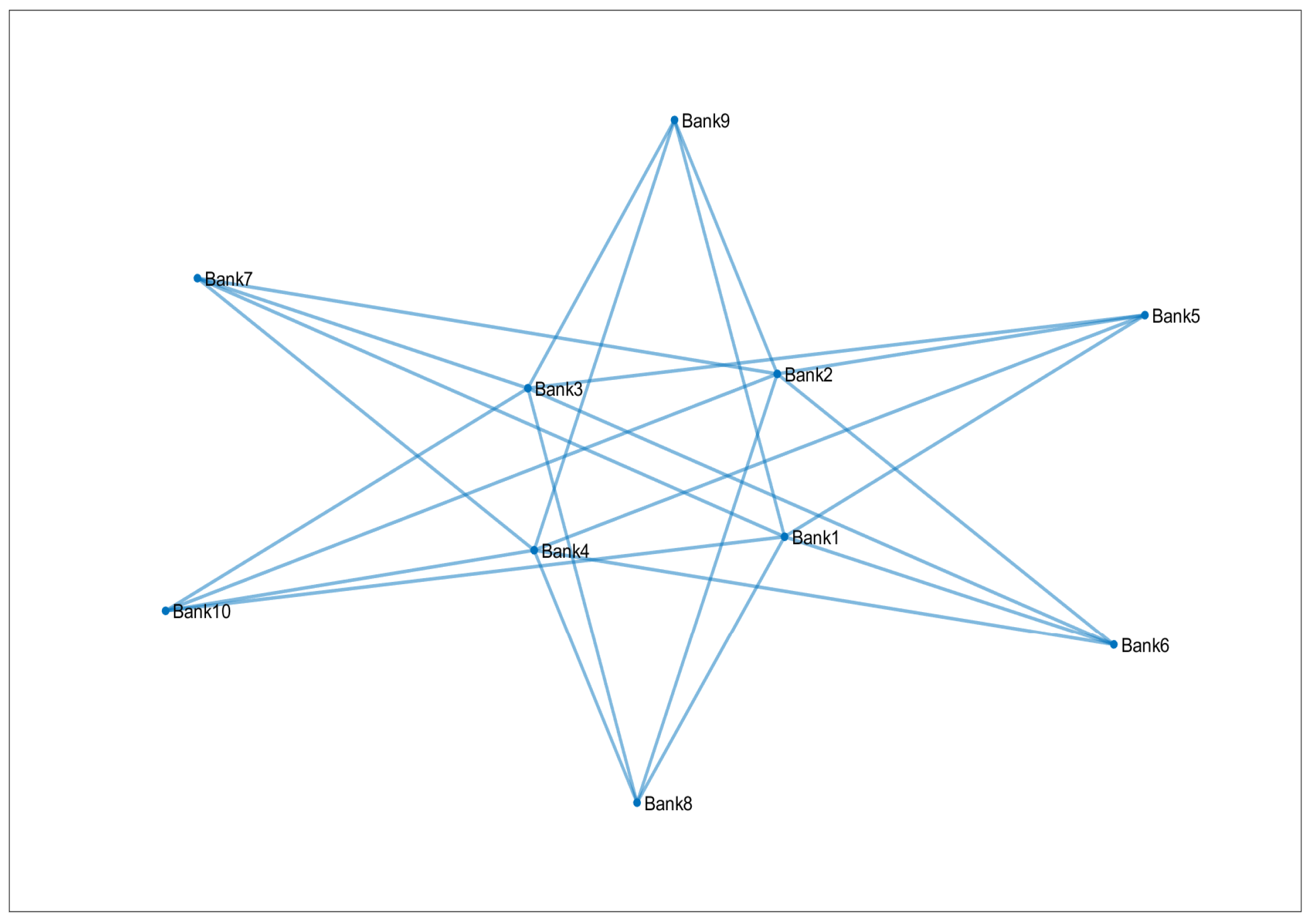
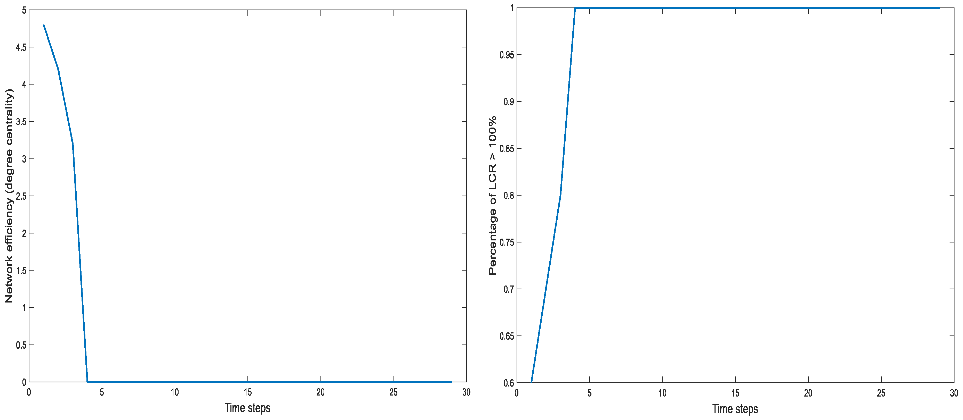
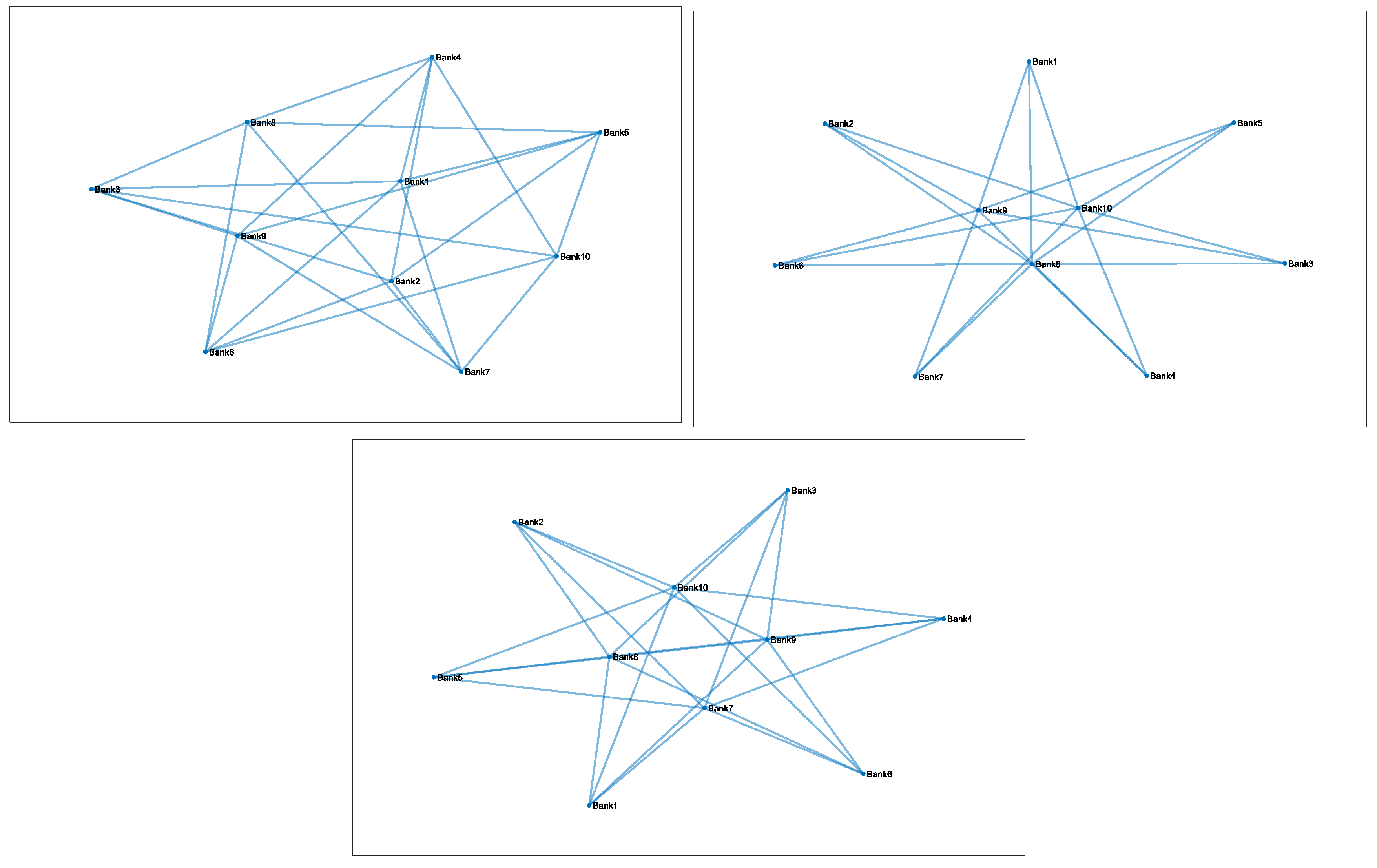
4. Numerical Experiment on Strategic Interbank Network Formation

“The socioeconomic perspective has emphasized understanding how the strategic behavior of the interacting agents is influenced by—and reciprocally shapes—relatively simple network architectures” [31]. We move in the direction pointed by the above authors in constructing some numerical experiments based on the KTAP model previously introduced, using the concept of strategic network formation.
Strategic network formation does not only face individual incentives of agents to form or severe links, but also provides the possibility to have measures of which networks might be considered “best” from the point of view of the overall welfare of the system [32]. In our model we each pair of functional subsystem is linked if trading occur between the two, based on the transition probabilities. Then, an unweighted and undirected network is formed at each time step.
Top ranked UK banks might be considered to be the following: HSBC Holdings, Barclay’s PLC, Royal Bank of Scotland, Lloyds Banking Group, Standard Chartered PLC, Santander UK, Nationwide Building Society, Schroders, Close Brothers and Coventry Building Society. We assume then that agents in our modelization are clusterized into 10 functional subsystems, here representing the banks. Loans, Treasury securities and reserves represent in general principal assets. For our numerical experiment we used 9 liquidity classes with the H Q L A cluster defined above, for each bank. The initial liquidity profile on each bank is then similar to the one in Figure 1. We have chosen the initial liquidity profile for each bank as randomly drawn from a normal distribution, using 1000 replications, with mean equal to 6 and standard deviation taking equally spaced values from 1 to 2, for the FS from 1 to 10, respectively. The liquidity profiles for the ten banks of the numerical experiment are represented in the following set of bar charts:
In our experiment, we assume that the net cash outflows for the involved banks is such that the liquidity ratio spans over an interval from 80% up to 125%. Given the liquidity profile graphically outlined in Figure 4 it is computed to assume the following values from the first to the 10-th bank
N C O F = 22 % , 20 % , 24 % , 24 % , 25 % , 20 % , 24 % , 25 % , 23 % , 19 % ,
expressed as percentages of the balance sheet for each FS. We are using the values obtained in Equation (14) for the net cash outflows of the ten banks.
We are now going to simulate the following dynamics for the liquidity profile of the ten banks. The initial conditions for the liquidity profiles are outlined graphically in Figure 4 and we are considering the net cash outflows of the ten banks (14) fixed over the time horizon of the numerical experiment n a first case study and then endogenously changing as an effect of the dynamics, in a second case study.
On each time step (daily) the liquidity profile is updated as a result of the financial interactions modelled as stochastic games of competition/cooperation triggered by the liquidity requirements quantified using the liquidity coverage ratio. Moreover, the intensity of the payoff is exogenously impactedby the Overnight London Interbank Offered Rate (LIBOR) (see Figure 5 for a graphical representation of the specific values used in the numerical experiments).We run the experiment in the time interval from 2 March 2020 to 1 April 2020, and on each day the liquidity profile of each bank is updated accordingly.
The initial network structure is represented in Figure 6.
By applying the individual incentives represented by the transition probabilities (4)–(9), the initial homogeneous network structure breaks down into a more and more sparse, hierarchical structure, represented by a core-periphery structure, until it reachs the empty network at the time horizon of the experiment (for a representation in terms of graphs see Figure 7).
Centrality measures on networks are strongly related to efficiency of the system in term of its, resilience and the individual payoffs of the agents [32]. There are different measures of the centrality of agents in a network, each of them actually based on some slight variation on nodal statistics, that is, vectors of data able to describe the position of a node in a given network. A centrality measure basically process this information producing a score for each node. In [32] it is discussed how the axioms underlying standard centrality measures (monotonicity, symmetry and additivity) may be easily compared with the way in which economists model time-discounted utility functions. Degree centrality, for instance, is measured by the number of links held by each node, but of course one can imagine different ways of processing the information. Specifically, degree centrality gives some insight into the connectivity of the node.
Inspired by [31], in our modellization, we measure network efficiency by the aggregate degree centrality of the nodes. Using this approach, we observe that the time evolution of the network structure is accompanied with a breakdown in network efficiency, graphically represented in Figure 8.
Although the percentage of nodes that satisfy the regulatory rule for the LCR increases from 50% up to 100%.

Case Study II: Penalty for Excesses of Liquidity Reserves

We are going to include in the model a penalty for subsystems holding excesses of liquidity reserves much above the regulatory threshold. Specifically, we assume a penalization for the nodes of the network that capitalize excesses of liquidity reserves such that L C R > 115 % , by assuming that such an LCR determines an increase of 5% in the Net Cash Outflow. Basically, at each time step of the numerical experiment, if the liquidity coverage ratio of a subsystem is such that L C R > 11 % the Net Cash Outflow is updated accordingly, with an increase of 5%.
The results of numerical simulations that follow have been obtained all else equal to the previous simulation, that is, the same initial liquidity profiles, the same time range of the interest rates, transition probabilities (4)–(9) and initial net cash outflows (14) for the ten banks.
The initial network structure, the same as that represented in Figure 6, is breaking into a more sparse, hierarchical structure, but after this transient state the same network structure is recovered such as at the initial time (a series of transient and final states are represented in Figure 9.
The time evolution of the network structure is again accompanied by a breakdown in network efficiency initially, when measured by aggregate degree centrality of the nodes, but soon after the network structure is recovered and stabilized (see Figure 10).
One might conclude that, all else equal, a penalization for holding excesses of reserves of liquidity is stabilizing the introduced network structure representing a stylized financial market.

5. Conclusions and Research Perspectives

In this paper, we have adopted the mathematical framework of the Kinetic Theory for Active Particles to model a complex adaptive network arising from basic financial interactions among a large number of agents clusterized in functional subsystems. The general mathematical structures allows for the possibility of including ’micro-macro’ interactions, that is, in which an agent might interact with one of the subsystems as a whole through its first moment of the distribution of the activity variable. This generalization involves an interesting research perspective in which the overnight interbank network of banks might play its role in the dynamics as well. In this paper we choose not to include the effect of heterogeneity by means of specific rules for the frequency of interactions, to highlight the main features of the models. However, introducing targeted rules for the frequency of interactions towards specific economic phenomenologies represents an interesting research path. However, an interesting research perspective would be that of considering different distribution of strategic behaviors of bank treasurers within the maintenance period, thus obtaining the same result in mean, but with liquidity profiles hugely different, inducing systemic risks. From the viewpoint of policies, widely used diagnostics on the complex adaptive networks arising from some simple rules at the level of economic agents might suggest policy prescriptions to improve network stability. In the illustrative examples of our paper, for instance, the numerical experiment suggests to lower the threshold for the net cash outflow, when the excesses reserves of liquidity of a financial institution are above a given prescribed limit, that, in the case of our numerical experiment, is represented by the 15% above the minimum requirement for the liquidity coverage ratio suggested by Basel III. Many different research perspectives arise from the above suggested modelization. Liquidity risk might strike without even the occurrence of actual loss, but jut due to the fear of its potential occurrence. By adopting such a view, one might introduce environmental volatility as in [31]. Another important questions applies in this framework—how far is illiquidity risk influenced by statistical properties of the interbank network? Moreover, the Basel ratio LCR has a major drawback: that it cannot be aggregated to provide a general view of the liquidity banking system risk in case of liquidity stress event. Would it work better to use the Liquidity Mismatch Index (LMI) introduced by [26]?

Author Contributions

Conceptualization, M.D., L.L. and E.M.; methodology, M.D., L.L. and E.M; software, M.D., L.L. and E.M.; validation, M.D., L.L. and E.M;writing—original draft preparation, M.D., L.L. and E.M; writing—review and editing, M.D., L.L. and E.M. All authors have read and agreed to the published version of the manuscript.

Funding

This research received no external funding.

Institutional Review Board Statement

Not applicable.

Informed Consent Statement

Not applicable.

Data Availability Statement

Not applicable.

Acknowledgments

The authors wish to thank the anonymous referees as they provided very valuable suggestions, a detailed review of the final draft of the paper and proposed interesting research perspectives as well and the editor of the Special Issue for the significant initiative.

Conflicts of Interest

The authors declare no conflict of interest.

Appendix A. Equilibrium Conditions for the Distribution of High Quality Liquid Assets on the Network

The present appendix is devoted to presenting a mathematical derivation of the time evolution of the percentage of high quality liquid assets (HQLA) on each subsystem, and on the network as a whole. Through differentiating Equation (3), applying the linearity property of derivatives and using Equation (1) one easily gets:
d H Q L A r ( t ) d t = i = 2 3 n n s = 1 M h , k = 1 n η h k r s [ f ] A h k r s ( h i ) ( f ) f h r f k s i = 2 3 n n f i r s = 1 M k = 1 n η i k r s [ f ] f k s , r = 1 , , M .
If, as we did in the numerical experiment, we assume that η h k r s = 1 , r = 1 , , M , i I , we easily get from Equation (A1):
d H Q L A r ( t ) d t = i = 2 3 n n s = 1 M h , k = 1 n A h k r s ( h i ) ( f ) f h r f k s H Q L A r ( t ) s = 1 M k = 1 n f k s , r = 1 , , M .
Finally, remembering that { f k s } k I is a probability distribution for each s node and then satisfies the property k = 1 n f k s = 1 , s = 1 , , M , we get the following result:
d H Q L A r ( t ) d t = i = 2 3 n n s = 1 M h , k = 1 n A h k r s ( h i ) ( f ) f h r f k s M · H Q L A r ( t ) ,
which gives a system of strongly coupled linear non-homogeneous system of ordinary differential equations, with the initial conditions H Q L A r ( t 0 ) , r = 1 , , M . Summing up over all the nodes in system (A3), leads to, after some small rearrangements:
d H Q L A ¯ ( t ) d t = H Q L A ¯ ( t ) + 1 M s , r = 1 M h , k = 1 n A h k r s ( h i ) ( f ) f h r ( t ) f k s ( t ) ,
where H Q L A ¯ ( t ) = 1 M r = 1 M H Q L A r ( t ) is the mean value of the percentage of high quality liquid assets over the network. The linear non-homogeneous ordinary differential Equation (A5) has an analytic solution, and gives a Cauchy problem when the initial condition H Q L A ¯ ( t 0 ) = 1 M r = 1 M H Q L A r ( t 0 ) although its explicit form might be difficult to be obtained in specific applications.
Necessary conditions for equilibrium of the mean of high quality assets on the newtork is then obtained for any t * such that
H Q L A ¯ ( t * ) = 1 M 2 s , r = 1 M h , k = 1 n A h k r s ( h i ) ( f ) f h r ( t * ) f k s ( t * ) .
Given that, in the first case study, the net cash outflows ( N C O F r , r = 1 , , r ) for each node of the network appears at the denominator in the definition of the liquidity coverage ratios (see Equation (2) and is assumed to be constant, the equilibrium condition (A5) applyes to the situation outlined in that case study. That is not the case instead for the second case study, where a penalty for excesses of reserves is included in the modelling framework that is determining, in general, time-depending net cash outflows for some nodes of the network. It is the opinion of the authors that the above short analytical considerations open research perspectives on the mathematical analysis of the modelling framework and results in specific case studies.

References

  1. Dolfin, M.; Leonida, L.; Outada, N. Modeling human behavior in economics and social science. Phys. Life Rev. 2017, 22, 1–21. [Google Scholar] [CrossRef] [Green Version]
  2. Dolfin, M.; Knopoff, D.; Limosani, M.; Xibilia, M.G. Credit risk contagion and systemic risk on networks. Mathematics 2019, 7, 1055. [Google Scholar] [CrossRef] [Green Version]
  3. Bellomo, N.; Bellouquid, A.; Gibelli, L.; Outada, N. A Quest Towards a Mathematical Theory of Living Systems; Birkhäuser; Springer: New York, NY, USA, 2017. [Google Scholar]
  4. Ajmone Marsan, G.; Bellomo, N.; Gibelli, L. Stochastic evolutionary differential games toward a systems theory of behavioral social dynamics. Math. Model. Methods Appl. Sci. 2016, 26, 1051–1093. [Google Scholar] [CrossRef]
  5. Kwon, H.R.; Silva, E.A. Mapping the Landscape of Behavioral Theories: Systematic Literature Review. J. Plan. Lit. 2019, 1051–1093. [Google Scholar] [CrossRef] [Green Version]
  6. Ball, P. Why Society Is a Complex Matter; Springer: Heidelberg, Germany, 2012. [Google Scholar]
  7. Burini, D.; De Lillo, S. On the complex interaction between collective learning and social dynamics. Symmetry 2019, 29, 967. [Google Scholar] [CrossRef] [Green Version]
  8. Lachowicz, M.; Leszczyński, H.; Puźniakowska–Galuch, E. Diffusive and anti-diffusive behavior for kinetic models of opinion dynamics. Symmetry 2019, 11, 1024. [Google Scholar] [CrossRef] [Green Version]
  9. Dolfin, D.; Leonida, L.; Muzzupappa, E. Forecasting Efficient Risk/Return Frontier for Equity Risk with a KTAP Approach: Case Study in Milan Stock Exchange. Symmetry 2019, 11, 1055. [Google Scholar] [CrossRef] [Green Version]
  10. Eftimie, R.; Gibelli, L. A kinetic theory approach for modelling tumour and macrophages heterogeneity and plasticity during cancer progression. Math. Model. Methods Appl. Sci. 2020, 30, 659–683. [Google Scholar] [CrossRef]
  11. Calvo, J.; Nieto, J.; Zagour, M. Kinetic Model for Vehicular Traffic with Continuum Velocity and Mean Field Interactions. Symmetry 2019, 11, 1093. [Google Scholar] [CrossRef] [Green Version]
  12. Aylaj, B.; Bellomo, N.; Gibelli, L.; Reali, A. On a unified multiscale vision of behavioral crowds. Math. Model. Methods Appl. Sci. 2020, 30, 1–22. [Google Scholar] [CrossRef]
  13. Bellomo, N.; Gibelli, L.; Outada, N. On the interplay between behavioral dynamics and social interactions in human crowds. Kinet. Relat. Mod. 2019, 12, 397–409. [Google Scholar] [CrossRef] [Green Version]
  14. Elaiw, A.; Al-Turki, Y.; Alghamdi, M. A critical analysis of behavioural crowd dynamics: From a modelling strategy to kinetic theory methods. Symmetry 2019, 11, 851. [Google Scholar] [CrossRef] [Green Version]
  15. Kim, D.; Quaini, A. A kinetic theory approach to model pedestrian dynamics in bounded domains with obstacles. Kinet. Relat. Mod. 2019, 12, 1273–1296. [Google Scholar] [CrossRef] [Green Version]
  16. Knopoff, D.; Nieto, J.; Urrutia, L. Numerical simulation of a multiscale cell motility model based on the kinetic theory of active particles. Symmetry 2019, 11, 1003. [Google Scholar] [CrossRef] [Green Version]
  17. Lachowicz, M.; Leszczyński, H. Modeling Asymmetric Interactions in Economy. Mathematics 2020, 8, 523. [Google Scholar] [CrossRef] [Green Version]
  18. Burini, D.; Chouhad, N. A Multiscale view of nonlinear diffusion in biology: from cells to tissues. Math. Model. Methods Appl. Sci. 2019, 11, 967. [Google Scholar] [CrossRef]
  19. Elaiw, A.; Al-Turki, Y. Particle methods simulations by kinetic theory models of human crowds accounting for stress conditions. Symmetry 2019, 12, 14. [Google Scholar] [CrossRef] [Green Version]
  20. Ardekani, A.M.; Distinguin, I.; Tarazi, A. Do banks change their liquidity ratios based on network characteristics? Eur. J. Oper. Res. 2020, 285, 789–803. [Google Scholar] [CrossRef]
  21. Bellomo, N.; Ha, S.-Y.; Outada, N. Towards a Mathematical Theory of Behavioral Swarms. ESAIM Control. Theory Var. Calc. 2020, 26, 125. [Google Scholar] [CrossRef]
  22. Knopoff, D.; Terna, P.; Secchini, V.; Virgillito, M.E. Cherry picking: consumer choices in swarm dynamics, considering price and quality of goods. Symmetry 2020, 12, 1912. [Google Scholar] [CrossRef]
  23. Pareschi, L.; Toscani, G. Interacting Multiagent Systems: Kinetic Equations and Monte Carlo Methods; Oxford University Press: Oxford, UK, 2013. [Google Scholar]
  24. Basel III: The Liquidity Coverage Ratio and Liquidity Risk Monitoring Tools; Bank for International Settlements: Basel, Switzerland, 2013.
  25. Principles for Sound Liquidity Risk Management and Supervision; Bank for International Settlements: Basel, Switzerland, 2008.
  26. Bai, J.; Krishnamurthy, A.; Weymuller, C.H. Measuring liquidity mismatch in the banking sector. J. Financ. 2018, LXXIII, 51–92. [Google Scholar] [CrossRef]
  27. Berger, A.N.; Bouwman, C.H.S. Bank Liquidity Creation and Financial Crises; Academic Press: Amsterdam, The Netherlands, 2015. [Google Scholar]
  28. Iori, G.; De Masi, G.; Precup, O.V.; Gabbi, G.; Caldarelli, G. A network analysis of the Italian overnight money market. J. Econ. Dyn. Control 2008, 32, 259–278. [Google Scholar] [CrossRef]
  29. Haldane, A. Rethinking the Financial Network, Speech by Mr Andrew G Haldane at at the Financial Student Association, Amsterdam, 28 April 2009. Available online: https://www.bis.org/review/r090505e.pdf (accessed on 26 November 2020).
  30. Stiglitz, J.E. The contributions of the economics of information to twentieth century economics. Q. J. Econ. 2000, 115, 1441–1478. [Google Scholar] [CrossRef]
  31. Schweitzer, F.; Fagiolo, G.; Sornette, D.; Vega-Redondo, F.; Vespignani, A.; White, D.R. Economic networks: the New Challenges. Science 2009, 325, 422–425. [Google Scholar] [CrossRef]
  32. Jackson, M.O. Social and Economic Networks; Princeton University Press: Princeton, NJ, USA; Oxford, UK, 2008. [Google Scholar]
Figure 1. An example of a liquidity profile with nine liquidity classes.
Symmetry 13 00363 g001
Figure 2. Pictorial representation of a dynamics of competition and a dynamics of cooperation, respectively.
Symmetry 13 00363 g002
Figure 3. ICE Benchmark Administration Limited (IBA), Overnight London Interbank Offered Rate (LIBOR), based on British Pound [GBPONTD156N], retrieved from FRED, Federal Reserve Bank of St. Louis; https://fred.stlouisfed.org/series/GBPONTD156N, accessed on 6 January 2021.
Symmetry 13 00363 g003
Figure 4. Initial liquidity profiles for the 10 banks of the numerical experiment.
Symmetry 13 00363 g004
Figure 5. ICE Benchmark Administration Limited (IBA), Overnight London Interbank Offered Rate (LIBOR), based on British Pound [GBPONTD156N], retrieved from FRED, Federal Reserve Bank of St. Louis; https://fred.stlouisfed.org/series/GBPONTD156N, accessed on 6 January 2021.
Symmetry 13 00363 g005
Figure 6. Initial network configuration.
Symmetry 13 00363 g006
Figure 7. Time evolution of the network configuration up to the time horizon of the experiment (from left to right) and on the second row.
Symmetry 13 00363 g007
Figure 8. Diagnostic of network robustness: time evolution of the network efficiency measured on the basis of the aggregate degree centrality of nodes (left) and of the percentage of nodes that satisfy the Liquidity Coverage Ratio (LCR) requirement (right).
Symmetry 13 00363 g008
Figure 9. Time evolution of the network configuration up to the time horizon of the experiment (from left to right) and on the second row.
Symmetry 13 00363 g009
Figure 10. Diagnostic of network robustness for case study 2: time evolution of the network efficiency measured on the basis of the aggregate degree centrality of nodes (left) and of the percentage of nodes that satisfy the Liquidity Coverage Ratio requirement (right).
Symmetry 13 00363 g010
Publisher’s Note: MDPI stays neutral with regard to jurisdictional claims in published maps and institutional affiliations.

