Article

A Model Free Adaptive Scheme for Integrated Control of Civil Aircraft Trajectory and Attitude

Institute of Advanced Control System, School of Electronic and Information Engineering, Beijing Jiaotong University, Beijing 100044, China
*
Author to whom correspondence should be addressed.
Symmetry 2021, 13(2), 347; https://doi.org/10.3390/sym13020347
Submission received: 7 January 2021 / Revised: 16 February 2021 / Accepted: 17 February 2021 / Published: 20 February 2021

Abstract

:
The adaptive trajectory and attitude control is essential for the four-dimensional (4D) trajectory operation of civil aircraft in symmetric thrust flight. In this work, an integrated trajectory and attitude control scheme is proposed based on the =multi-input multi-output (MIMO) model free adaptive control (MFAC) method. First, the full-form dynamic linearization technique is adopted to build the equivalent data model of aircraft. Also, the MIMO MFAC scheme with saturation constraint is designed to achieve an accurate tracking control for a given 4D trajectory and attitude. Besides, the performance limitations of aircraft are taken into consideration, and the MIMO MFAC scheme with hard constraints is designed. In addition, to improve the simulation efficiency, a control scheme with mixed constraints, i.e., saturation and hard constraints, is further proposed. It can be seen from the simulation results that the proposed method can perform an integrated control of the aircraft 4D trajectory and attitude without precise modeling, and the control performance is better than that of the model-based control method in terms of flight altitude and yaw angle control. The integrated data-driven control scheme proposed in this paper provides a theoretical solution for the precise operation of aircraft under 4D trajectory.

1. Introduction

With the sustained and rapid development of the air transport industry, air traffic operation and management is confronted with various pressures and challenges. To deal with the current and future air traffic problems, the United States proposed a project named Next Generation Air Traffic Transportation System (NextGen) [1], and Eurocontrol launched a program called Single European Sky Air Traffic Management Research (SESAR) [2]. Both of them rely on trajectory-based operation to improve the safety, efficiency and capacity of air traffic operation. To achieve this goal, each aircraft is required to equip with 4D trajectory automatic guidance and control, including trajectory tracking and attitude control. Therefore, the research on adaptive trajectory tracking and attitude control methods for precise 4D trajectory operation is essential for realizing safe, green and efficient air traffic operations.
The existing research work mainly explores trajectory tracking control, attitude control and trajectory-attitude control. For trajectory tracking control, the commonly used methods include feedback and feedforward control [3], backstepping control [4,5,6,7,8], model predictive control [9,10] and so on. In the literature [3], the feedback and the feedforward control law are designed based on the minimum phase and the non-minimum phase dynamics models of the aircraft, respectively. The backstepping control method combines the aircraft dynamics model with the disturbance observer [6] or the extended state observer [7] to compensate for external disturbances. For the model predictive control method, the low-order equivalent system model of the aircraft must be established first. Then the method is used to realize the trajectory tracking control of the Unmanned Aerial Vehicle (UAV) in the two-dimensional plane [10]. To improve the robustness of control, the uncertainty and external disturbances of the observer estimation model are introduced [11,12]. In addition, the literature [13,14,15] employs the stable inversion and iterative learning control methods to tackle the aircraft trajectory tracking problem during the phase of landing, continuous climbing and continuous descending.
In terms of aircraft attitude control, the commonly used methods include sliding mode control [16,17], model predictive control [18], active disturbance rejection control [19,20], dynamic inversion control [21] and so on. In these studies, accurate aircraft dynamics models are usually used, where the aerodynamic coefficients need to be obtained through wind tunnel experiments and flight tests [18]. To overcome the difficulty of accurate modeling, a PID control method with gain adjustment for the fixed-wing UAV attitude control was proposed in the work [22]. Also, the authors in [23] established a model free adaptive attitude control method for launching the vehicle. In addition, the attitude control of aircraft under high angle of attack when the stall occurs and attitude control of a structurally damaged aircraft were respectively studied in [24,25].
Currently, there are few studies that consider both trajectory tracking and attitude control in the 4D trajectory operation, and the existing research is mainly divided into separate control and integrated control for this problem. In terms of separate control, the literature [26] achieves separate control of trajectory and attitude following the feedforward H and dynamic inversion control methods. In the research of [5], indirect and direct NLI (Non-Linear Inversion) control methods are used respectively to realize aircraft trajectory control. Also, backstepping and NLI methods are used to perform attitude control. For integrated control, the trajectory tracking and attitude control of vertical take-off and landing aircraft was studied in [11], using the model predictive control method. In the work of [27] the controller is designed based on the small disturbance linearized aircraft dynamics model and the linear Gaussian quadratic method. In this case, the position error and the slip angle error of the aircraft tend to be zero under atmospheric disturbance. Although these methods have achieved good simulation results, they all need an accurate mechanism modeling, such as establishing the small disturbance linearization model or the aircraft dynamics model. Therefore, these studies are faced with two problems: one is that the accurate mechanism model is difficult to establish; the other is that there are a lot of aerodynamic parameters in the model, which are usually obtained indirectly through experiment, simulation and data fitting. Specifically, the impact of these unknown and time-varying aerodynamic parameters is already reflected in the input and output data of the system. In contrast, the data-driven control method can avoid the complex system modeling and can make full use of the I/O data to achieve a desired control quality.
As for the data-driven control, the controller design does not include the mathematical model information of controlled process, and only the online and offline I/O data of the control system and the knowledge obtained through data processing are used to design the controller. Also, under certain assumptions, the stability, convergence and robustness of the controller can be guaranteed by some control theories and methods [28]. At present, the domestic and overseas data-driven control methods include: Simultaneous Perturbation Stochastic Approximation (SPSA), Model Free Adaptive Control (MFAC), Unfalsified Control (UC), PID control, Iterative Feedback Tuning (IFT), Virtual Reference Feedback Tuning (VRFT), etc. In contrast, the model-free adaptive control has a complete mathematical theoretical foundation with strict proof of stability and convergence [29,30,31]. Owing to the dynamic linearization method in MFAC, the controller structure can be determined relatively easily. The review of MFAC can be found in the literature [32,33,34]. At present, the model-free adaptive control method and its improved versions have been widely used in electromagnetic control [35], vibration control [36], water level control [37], electric energy control [38], traffic road network boundary control [39] and other fields. Meanwhile, recent research extended the application of model free adaptive control theory to trajectory-based aircraft operation [40].
Motivated by the above research, the multi-input multi-output (MIMO) model free adaptive control method is adopted in this paper to design a framework for integrated control of 4D trajectory and attitude. Compared with the existing research work, the main contributions of this paper are as follows: (1) Compared with the model-based control method proposed in the research of [5,41], the data-driven control method proposed in this paper does not need accurate modeling of aircraft motion process and data fitting of various aerodynamic parameters. Instead, the input and output data of the control system are directly used to design the controller. (2) Compared with the existing research work based on the model-free adaptive control [23,40], the performance limitations of aircraft are considered in this paper, making the proposed control method more applicable to the actual operation of civil aircraft. (3) Compared with the state-of-art integrated control method of civil aircraft [27], the roll, pitch, yaw angle and flight positions of the aircraft instead of the disturbance of these variables [27] are directly controlled in the proposed method, contributing to more intuitive control object and simulation results in this paper.
The rest of this paper is organized as follows: In Section 2 the aircraft motion model is used to generate I/O data. In Section 3 the MIMO MFAC method with saturation constraints is designed. In Section 4, the MIMO MFAC method with hard constraints is proposed considering the aircraft performance limitations. Furthermore, a control scheme with mixed constraints is proposed in Section 5. In Section 6, simulation experiments are carried out to verify effectiveness of the proposed method, and the conclusion is given in Section 8.

2. Data Generation

The I/O data of aircraft operation in symmetric thrust flight is generated by Equations (1)–(13) [41]. Some related factors behind these equations, such as assumptions, force diagram, wind effect, engine alignment and sideslip effect, are explained in detail in the work of [5]. Since these equations are used only to generate I/O data in our research and are not involved in the design of control algorithms, the derivation of these equations is omitted here.
Aircraft longitudinal motion equations:
γ ˙ = 1 m V a L + F t h r sin ( α ) m g cos ( γ ) q V w x cos ( α ) + V w z sin ( α ) V a + 1 V a V ˙ w z cos ( α ) V ˙ w x sin ( α )
V ˙ a = 1 m F t h r cos ( α ) D m g sin ( γ ) + q V w x sin ( α ) V w z cos ( α ) V ˙ w x cos ( α ) V ˙ w z sin ( α )
x ˙ E = V a cos ( γ ) cos ( ψ ) + V w x cos ( θ ) cos ( ψ ) + V w z sin ( θ ) cos ( ψ )
z ˙ E = V a sin ( γ ) V w x sin ( θ ) + V w z cos ( θ )
θ ˙ = q
q ˙ = M B
M = 1 2 ρ S V a 2 c ¯ C m + c ¯ C m δ e l e δ e l e
Aircraft lateral motion equations:
y ˙ E = V a cos ( γ ) sin ( ψ ) + V w x cos ( θ ) sin ( ψ ) + V w y cos ( ψ ) + V w z sin ( θ ) sin ( ψ )
ϕ ˙ = p
ψ ˙ = r cos ( ϕ )
p ˙ = 1 A C E 2 ( C L r + E N )
r ˙ = 1 A C E 2 ( E L r + A N )
L r N = 1 2 ρ S V a 2 b C l b C n + b C l δ a i l 0 b C l δ r u d b C n δ a i l 0 b C n δ r u d δ a i l δ r u d
The parameters and their meanings in the model are as follows:
γ represents the flight path angle (deg);
m represents the mass of the aircraft (kg);
V a represents the speed of the aircraft (m/s);
F t h r represents the thrust of the aircraft (N);
α represents the angle of attack of the aircraft (deg);
g represents the acceleration of gravity ( m / s 2 );
V w x , V w y , V w z respectively represent the components of wind speed in the directions of x , y , z (m/s);
ϕ , θ , ψ represent the roll, pitch and yaw angle of the aircraft respectively (deg);
p , q , r represent the roll, pitch and yaw angular velocity of the aircraft respectively (deg/s);
L r , M , N represent roll, pitch and yaw moment respectively (N·m);
ρ represents air density ( kg / m 3 );
S represents the wing area ( m 2 );
c ¯ represents the average chord length (m);
C l , C m , C n represent the aerodynamic coefficients of roll, pitch and yaw respectively;
C l δ a i l represents the roll caused by the aileron deflection coefficient ( rad 1 );
C l δ r u d represents the roll caused by the rudder deflection coefficient ( rad 1 );
C m δ e l e represents the pitch caused by the elevator deflection coefficient ( rad 1 );
C n δ a i l represents the yaw caused by the aileron deflection coefficient ( rad 1 );
C n δ r u d represents the yaw caused by the rudder deflection coefficient ( rad 1 );
A , B , C , E represent the inertial matrix components ( kg · m 2 );
δ a i l , δ e l e , δ r u d represent the deflection angle of the aileron, elevator and rudder respectively (deg).
One of the difficulties faced by model-based control methods is to determine various aircraft performance parameters. Although some parameters can be found in the aircraft manual, there are still some aerodynamic parameters that are difficult to obtain, such as roll aerodynamic coefficient C l , pitch aerodynamics Coefficient C m and yaw aerodynamic coefficient C n . In the literature [5] the numerical calculation method of these parameters is given, as shown in Formula (14).
C l C m C n = C l β β + C l p b p 2 V a + C l r b r 2 V a C m 0 + C m α α + C m q c q 2 V a C n β β + C n p b p 2 V a + C n r b r 2 V a
where C l β , C l p , C l r , C m α , C m q , C n β , C n p , C n r are called non-dimensional stability derivatives, which are unknown nonlinear time-varying parameters. The values of these parameters depend on the aircraft and its angle of attack. In practice, the value of these non-dimensional stability derivatives can be obtained from fluid dynamics calculations, wind tunnel experiments and aircraft performance databases. However, restricted by many factors such as professional knowledge and experimental conditions, these methods may not be feasible in research. For this reason, a neural network model for each non-dimensional stability derivative is established in the literature [5]. The model extracts the relationship between the non-dimensional stability derivative and the angle of attack, and then it is used for the flight control and the simulation of a six-degree-of-freedom aircraft. Although this method achieves good simulation results, it suffers from a large modeling workload and a high dependence on the model. In this case, the aircraft dynamic model is regarded as a “black box” model in this research. Based on the analysis of the dynamic linearization relationship between the input and output data, an adaptive integrated scheme for trajectory and attitude control is constructed to realize the data-driven control of civil aircraft in 4D trajectory operation.

3. MIMO MFAC Method with Saturation Constraint

It can be seen from Equations (1)–(13) that the aircraft motion system is a MIMO nonlinear system, in which the aileron deflection angle δ a i l , the elevator deflection angle δ e l e , rudder deflection angle δ r u d , thrust F t h r and flight path angle γ are the inputs of the system, so define u = [ δ a i l , δ e l e , δ r u d , F t h r , γ ] T . Roll angle ϕ , pitch angle θ , yaw angle ψ , the position of the aircraft in the x , z axis direction x E , z E are the output of the system, so define y = [ ϕ , θ , ψ , x E , z E ] T . There is a coupling between the input and output variables of the system, which increase the complexity of the control problem. For this reason, the full-format dynamic linearization (FFDL) method is first adopted to obtain the equivalent data model of the controlled system at the current operating point, as shown below:
Δ y ( k + 1 ) = Φ f , L y , L u ( k ) Δ H L y , L u ( k )
where Φ f , L y , L u ( k ) = [ Φ 1 ( k ) Φ L y + L u ( k ) ] R m × ( m L y + m L u ) is the pseudo partitioned Jacobian matrix (PPJM), and the ith corresponding sub-matrix is denoted as follows.
Φ i ( k ) = ϕ 11 i ( k ) ϕ 12 i ( k ) ϕ 1 m i ( k ) ϕ 21 i ( k ) ϕ 22 i ( k ) ϕ 2 m i ( k ) ϕ m 1 i ( k ) ϕ m 2 i ( k ) ϕ m m i ( k ) R m × m , i = 1 , , L y + L u ,
Δ H L y , L u ( k ) = [ Δ y T ( k ) , , Δ y T ( k L y + 1 ) , Δ u T ( k ) , , Δ u T ( k L u + 1 ) ] T
where Δ ( y ) and Δ ( u ) are the vectors composed of system output increment and input increment, respectively, and L y and L u are the linearization length constant of output and input, respectively.
The objective of the aircraft trajectory and attitude integrated control is to make the error between the system output and the desired output as small as possible, and considering the physical limitations of the aircraft operation, the control input should not change too much. Therefore, it is necessary to satisfy the following control input criterion function.
J ( u ( k ) ) = y * ( k + 1 ) y ( k + 1 ) 2 + λ u ( k ) u ( k 1 ) 2
where y * ( k + 1 ) represents the expected output at time k + 1 , and λ > 0 is a weighting factor.
Substitute Formula (15) into (18), take the derivative of u ( k ) and make the derivative equal to zero, we can get
u ( k ) = u ( k 1 ) + λ I + Φ L y + 1 T ( k ) Φ L y + 1 ( k ) 1 Φ L y + 1 T ( k ) × y * ( k + 1 ) y ( k ) i = 1 L y Φ ^ i ( k ) Δ y ( k i + 1 ) i = L y + 2 L y + L u Φ ^ i ( k ) Δ u ( k i + L y + 1 )
Since Formula (19) contains an inversion term, when the input and output dimensions of the system are large, the inversion operation is very time-consuming and not suitable for practical use, so the following simplified algorithm should be used.
u ( k ) = u ( k 1 ) + Φ L y + 1 T ( k ) ρ L y + 1 y * ( k + 1 ) y ( k ) λ + Φ L y + 1 ( k ) 2 Φ L y + 1 T ( k ) i = 1 L y ρ i Φ i ( k ) Δ y ( k i + 1 ) λ + Φ L y + 1 ( k ) 2 Φ L y + 1 T ( k ) i = L y + 2 L y + L u ρ i Φ i ( k ) Δ u ( k i + L y + 1 ) λ + Φ L y + 1 k 2
where ρ ( 0 , 1 ] is the added step factor, which makes the algorithm more flexible, and i = 1 , 2 , , L y + L u . On the right side of the above equation, the second item is an error feedback item, and the third and fourth items are compensation items. Through error feedback and compensations at every moment, the optimal control input at the current moment is obtained.
Denote the maximum value of control input at time k as
u max ( k ) = [ δ a i l max , δ e l e max , δ r u d max , F t h r max , γ max ] T
and the minimum value of control input at time k as
u min ( k ) = [ δ a i l min , δ e l e min , δ r u d min , F t h r min , γ min ] T
To ensure that the control input does not exceed the upper and lower boundaries allowed by the system, the following saturation constraints are imposed on the control input.
Sat u ( k ) = u max ( k ) , if u ( k ) > u max ( k ) u ( k ) , if u min ( k ) u ( k ) u max ( k ) u min ( k ) , if u ( k ) < u min ( k )
Since the value of Φ in Formula (20) is unknown, Formula (20) cannot be used directly. Therefore, the projection algorithm is used to estimate the value of pseudo partitioned Jacobian matrix Φ f , L y , L u ( k ) .
Φ ^ f , L y , L u ( k ) = Φ ^ f , L y , L u ( k 1 ) + Δ y ( k ) Φ ^ f , L y , L u ( k 1 ) Δ H L y , L u ( k 1 ) × Δ H L y , L u T ( k 1 ) μ + Δ H L y , L u ( k 1 ) Δ H L y , L u T ( k 1 ) 1
To reduce calculation time and facilitate practical applications, the following simplified estimation algorithm should be used:
Φ ^ f , L y , L u ( k ) = Φ ^ f , L y , L u ( k 1 ) + η Δ y ( k ) Φ ^ f , L y , L u ( k 1 ) Δ H L y , L u ( k 1 ) Δ H L y , L u T ( k 1 ) μ + Δ H L y , L u ( k 1 ) 2
where η ( 0 , 2 ] is the step factor added to make the algorithm more flexible. Φ ^ f , L y , L u ( k ) = [ Φ ^ 1 ( k ) , Φ ^ 2 ( k ) , , Φ ^ L y + L u ( k ) ] R m × m ( L y + L u ) is the estimated value of Φ f , L y + L u ( k ) . For the ith sub-matrix, the estimated value is as follows.
Φ ^ i ( k ) = ϕ ^ 11 i ( k ) ϕ ^ 12 i ( k ) ϕ ^ 1 m i ( k ) ϕ ^ 21 i ( k ) ϕ ^ 22 i ( k ) ϕ ^ 2 m i ( k ) ϕ ^ m 1 i ( k ) ϕ ^ m 2 i ( k ) ϕ ^ m m i ( k ) R m × m , i = 1 , , L y + L u ,
It should be noted that the pseudo partitioned Jacobian matrix Φ f , L y , L u ( k ) contains very complex system dynamics at the moment k, and its value is estimated based on the input and output data of the system in the present and the past. In the literature [5], the system dynamics are calculated through neural network data fitting and accurate modeling. It can be seen that the data-driven control algorithms are fundamentally different from the model-based control algorithms for dealing with complex system dynamics. For the data-driven control method, the I/O data rather than the mathematic model are used to reflect the system dynamics, avoiding the difficulty of accurate modelling and unmodeled dynamics.

4. MIMO MFAC Method with Hard Constraints

In the integrated control of aircraft trajectory and attitude, the control variables, such as deflection angle of control surface, thrust, and flight path angle, have a certain range of variation. At the same time, the rate of variation cannot be too large considering the stability of flight and the constraints of aircraft performance. Based on the above analyses, the integrated control of aircraft trajectory and attitude with hard constraints, including limited control input and control input increment, is designed as follows.
First, limit the input increment at time k to be within the specified range. The inequality constraints are as follows.
Δ u ( k ) Δ u max
Δ u ( k ) Δ u min
Second, limit the input amplitude at time k within the specified range. The inequality constraints are as follows.
u ( k ) u ( k 1 )     u max u ( k 1 )
u ( k ) u ( k 1 )     u min u ( k 1 )
In matrix form, the above inequality can be written as follows.
I I I I Δ u ( k ) Δ u max Δ u min ( u max u ( k 1 ) ) u min u ( k 1 )
Finally, the data model (15) is substituted into the control input criterion function (18). After some deductions, the quadratic performance index can be obtained. Combined with the above linear inequality constraints, the constrained quadratic programming problem can be written as follows.
min Δ u ( k ) 1 2 Δ u T ( k ) H ( k ) Δ u ( k ) + G T ( k ) Δ u ( k ) s . t . C u Δ u ( k ) b u ( k )
where
H ( k ) = Φ ^ L y + 1 T ( k ) Φ ^ L y + 1 ( k ) + λ I
G ( k ) = 2 Φ ^ L y + 1 T ( k ) ( y * ( k + 1 ) y ( k ) i = 1 L y Φ ^ i ( k ) Δ y ( k i + 1 ) i = L y + 2 L y + L u Φ ^ i ( k ) Δ u ( k i + 1 + L y ) )
C u = I I I I , b u ( k ) = Δ u max Δ u min ( u max u ( k 1 ) ) u min u ( k 1 )
By using an appropriate quadratic programming solver, the solution of Equation (30) can be easily obtained, which is the optimal control input within the specified range.

5. Control Scheme with Mixed Constraints

To speed up the simulation, the control methods with hard constraints and saturation constraint can be combined to form a data-driven control scheme with mixed constraints based on full-format dynamic linearization. The specific steps are as follows.
Given time k 1 , when k k 1 , using a suitable solver to solve Equation (30); when k > k 1 , perform the following steps:
(1)
Estimate the value of PPJM Φ f , L y + L u ( k ) by Formula (23).
(2)
Reset the value of Φ ^ L y + 1 ( k ) when the following conditions are satisfied:
if | ϕ ^ i i ( L y + 1 ) ( k ) | < b 2 or | ϕ ^ i i ( L y + 1 ) ( k ) | > α b 2 or sign ( ϕ ^ i i ( L y + 1 ) ( k ) ) sign ( ϕ ^ i i ( L y + 1 ) ( 1 ) ) , i = 1 , , m , then
ϕ ^ i i ( L y + 1 ) ( k ) = ϕ ^ i i ( L y + 1 ) ( 1 )
if | ϕ ^ i j ( L y + 1 ) ( k ) | > b 1 or sign ( ϕ ^ i j ( L y + 1 ) ( k ) ) sign ( ϕ ^ i j ( L y + 1 ) ( 1 ) ) , i , j = 1 , , m , i j , then
ϕ ^ i j ( L y + 1 ) ( k ) = ϕ ^ i j ( L y + 1 ) ( 1 )
where b 1 is a small value, and α 1 , b 2 > b 1 ( 2 α + 1 ) ( m 1 ) . ϕ ^ i j ( L y + 1 ) ( 1 ) is the initial value of ϕ ^ i j ( L y + 1 ) ( k ) .
(3)
Calculate the current control input using the estimated value of PPJM Φ f , L y + L u ( k ) .
u k = u k 1 + Φ ^ L y + 1 T k ρ L y + 1 y * k + 1 y k λ + Φ ^ L y + 1 k 2 Φ ^ L y + 1 T k i = 1 L y ρ i Φ ^ i k Δ y k i + 1 λ + Φ ^ L y + 1 k 2 Φ ^ L y + 1 T ( k ) i = L y + 2 L y + L u ρ i Φ ^ i k Δ u k i + L y + 1 λ + Φ ^ L y + 1 k 2
i , j = 1 , , m ; ρ 1 , , ρ L y + L u ( 0 , 1 ] ; η ( 0 , 2 ] ; λ > 0 , μ > 0 . According to Equation (21), impose the saturation constraint on the control input.
The proposed method is a data-driven approach, since only input and output data are used in the control scheme, and no model information is used. Due to its model-free characteristics, the possible uncertainties presented in the dynamic model, such as those related to inertia characteristics or aerodynamic derivatives, may not affect its control performance. In this sense, the proposed method should have strong robustness in dealing with complex system control problems.

6. Simulation Results

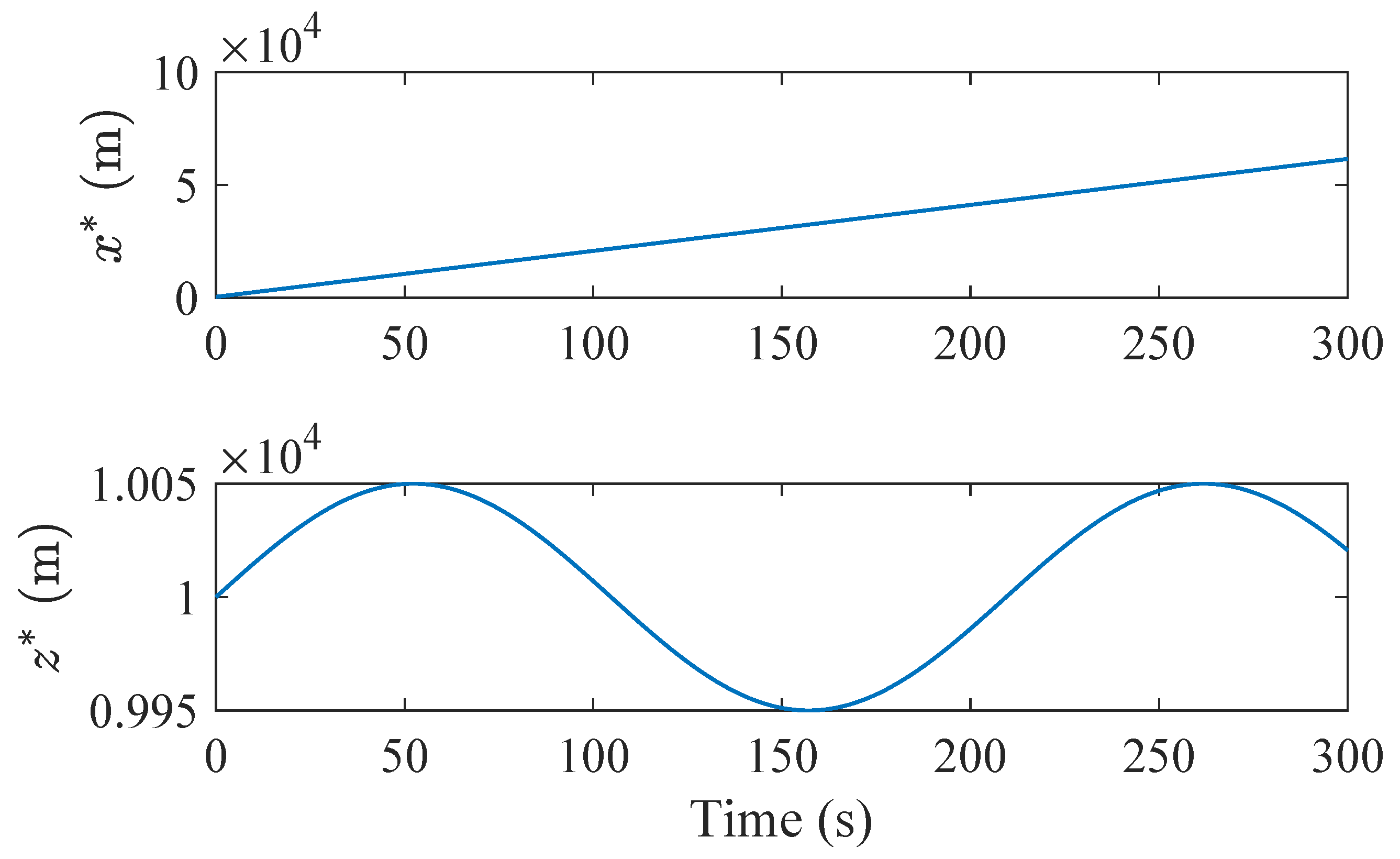
In this section, we will verify the correctness of the proposed method through numerical simulation for the integrated control of aircraft trajectory and attitude. Assuming that the aircraft moves along the x axis and needs to perform a sinusoidal motion with an amplitude of 50 m in the z axis direction. The desired trajectories are shown in Figure 1. To achieve this kind of operation, the aircraft needs to adjust the flight attitude at the same time. The desired roll, pitch and yaw angle are shown in Figure 2.
To facilitate comparison, the NLI method used in the literature [5] will be used for simulation in this section. NLI method needs to establish the following equations according to the mechanism model of aircraft.
m τ V ( V a d V a ) + m g sin ( γ ) = F t h r cos ( α ) D ( ρ , α , V a )
m V a τ γ ( γ d γ ) + m g cos ( γ ) = F t h r sin ( α ) + L ( ρ , α , V a )
arctan V a g τ ψ ( ψ d ψ ) = ϕ
By solving Equations (34)–(36), the thrust F t h r , the angle of attack α and the roll angle ϕ can be obtained. These values are further substituted into the aircraft dynamic model to calculate the position of the aircraft. For the attitude of the aircraft, according to the NLI method adopted in the work [5], the deflection angle of the aircraft control surface (aileron, elevator, rudder) at each time can be obtained. In the following simulation, this method is referred to as NLI, and the method proposed in this paper is referred to as FFDL-MFAC.
To facilitate simulation, the Euler discretization method is used to discretize Equations (1)–(13).The sampling interval is 0.01 s, and the control input is selected as u ( k ) = [ δ a i l ( k ) , δ e l e ( k ) , δ r u d ( k ) , F t h r ( k ) , γ ( k ) ] T , control output y ( k ) = [ ϕ ( k ) , θ ( k ) , ψ ( k ) , x E ( k ) , z E ( k ) ] T .
The parameters of the aircraft and controller used in the simulation are shown in Table 1. Let the thrust of the aircraft at the initial moment be F t h r ( 1 ) = 30,000 N and the speed V a ( 1 ) = 200 m / s . Set the deflection angle of each control surface and the attitude angles are 0 at the initial moment, and the value of the pseudo partitioned Jacobian matrix at the initial moment is as follows:
Φ ^ 1 ( 1 ) = 0.7400 0 0.1480 0 0 0 53.1875 0 0.0009 0 0 0 0 0 0 0 0 0 16.5319 0 0 0 0 747.4000 814.0000
Φ ^ 2 ( 1 ) = 1.4800 0 0 0 0 0 55.5000 0 0 0 0 0 2.4667 0 0 0 0 0 15.7447 0 0 0 0 740 740
Φ ^ 3 ( 1 ) = 0.5 0 0 0 0 0 0.8 0 0.00 0 0 0 0.6 0 0 0 0 0 0.47 0 0 0 0 0.0 0.0001
The change range of the control input increment and the control input within the sampling interval is shown in Table 2.
The simulation results are shown in Figure 3, Figure 4, Figure 5, Figure 6, Figure 7 and Figure 8. 
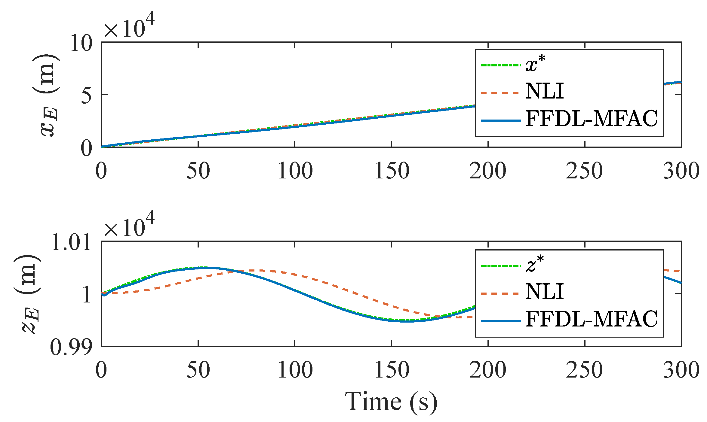
Figure 3 shows the result of trajectory tracking with mixed constraints. It can be seen that the FFDL-MFAC method with mixed constraints achieves an accurate trajectory tracking. Also, it is noted that the proposed method achieves a better control performance than the NLI method for the tracking of z coordinates.
Figure 4 exhibits the results of aircraft attitude control. It can be seen that the proposed method achieves a better tracking performance of the yaw angle ψ than the NLI method. Although some fluctuations exist in the attitude output before an accurate tracking is achieved, these fluctuations are within an acceptable range, and the desired tracking effect is soon achieved. The reasons for these fluctuations may be twofold. On the one hand, the initial values of the controller parameters may not be set accurately. On the other hand, the controller only uses a small amount of current and past I/O data without the model information when the aircraft changes its flight state.
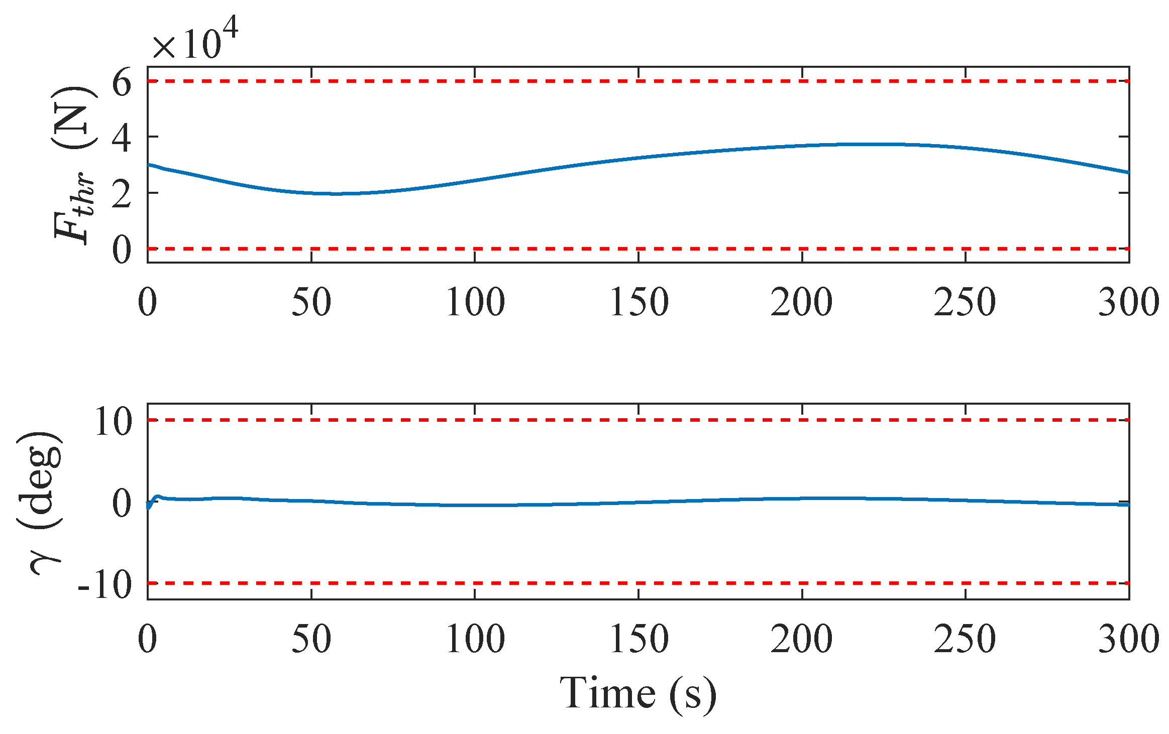
Figure 5, Figure 6, Figure 7 and Figure 8 respectively illustrate the control input and the increment of control input in the simulation with mixed constraints, where the red dotted line represents the upper and lower boundaries of input or input increment. It can be seen from Figure 5 and Figure 6 that the aircraft’s thrust, flight path angle, and control surface deflection angle are all within the boundaries. Although the aileron deflection angle and rudder deflection angle fluctuate before an accurate tracking is achieved, they are within the acceptable range.
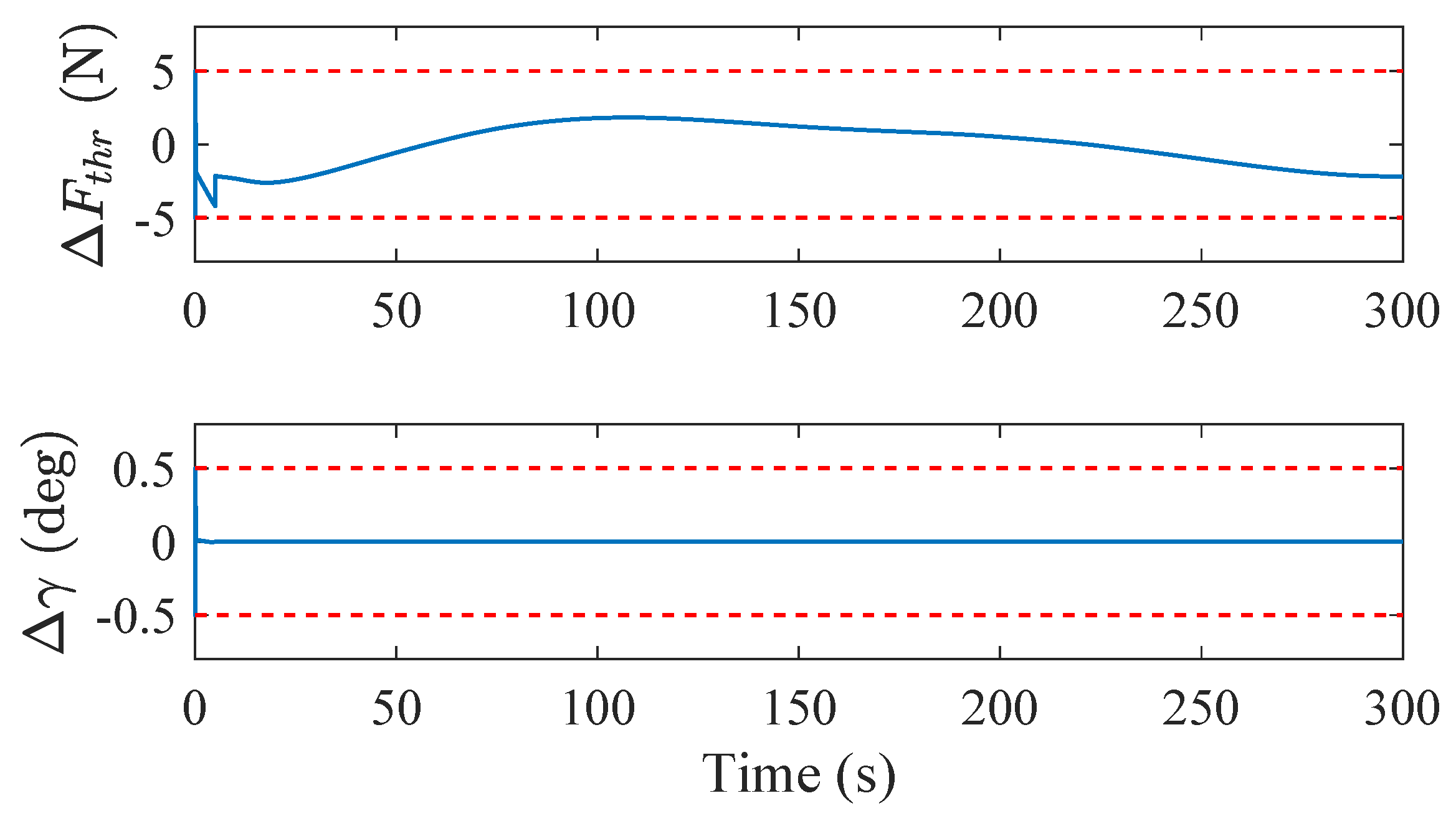
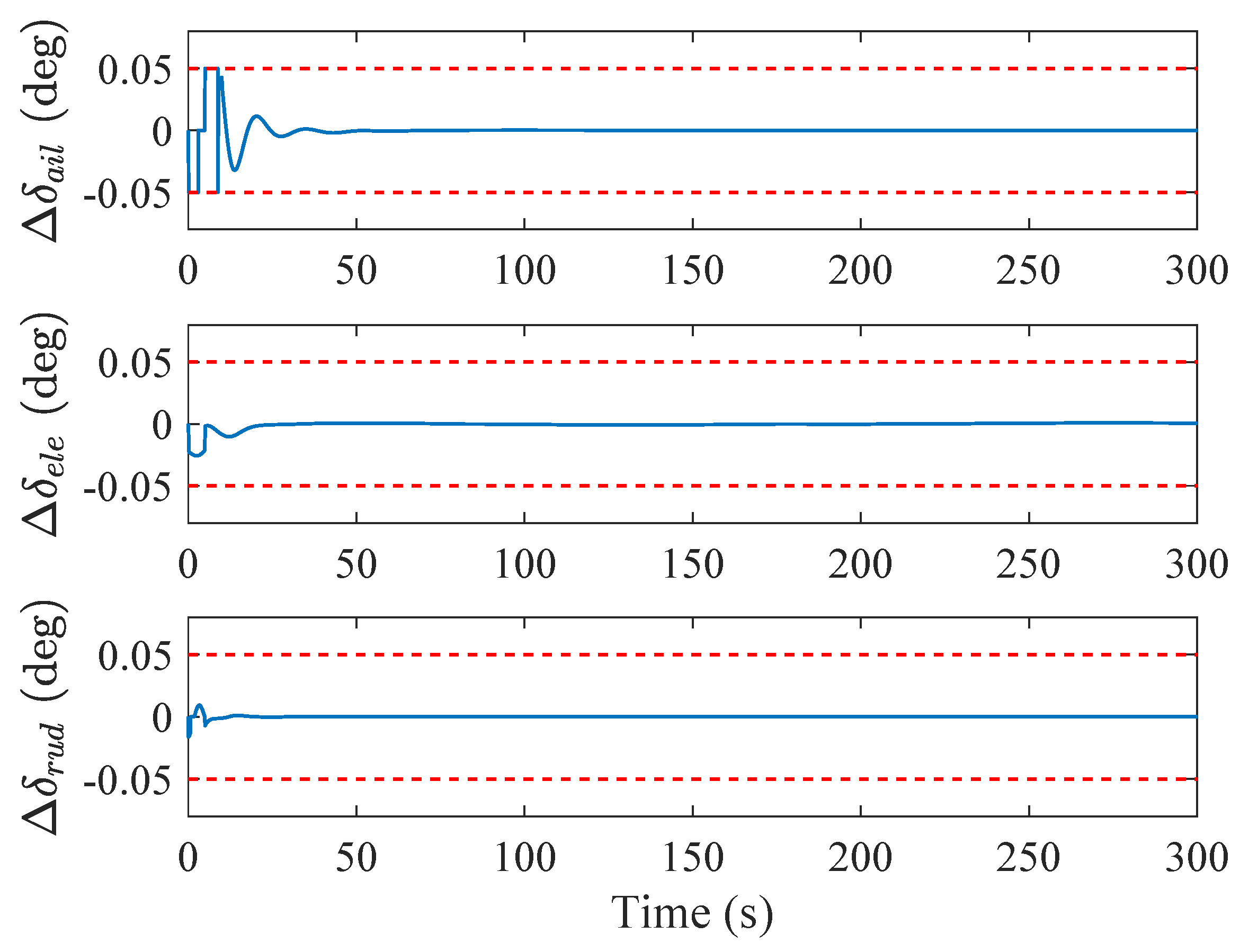
From Figure 7 and Figure 8, it can be seen that the aircraft’s thrust increment, flight path angle increment, and control surface deflection angle increment are all within the boundaries. Also, fluctuation ranges of these parameters are all within the acceptable range.

7. Discussion

To clearly show the control performance of proposed method and NLI method, two numerical indicators are adopted, namely the root mean square (RMS) e R M S = 1 n k = 1 n e ( k ) 2 for tracking error and total sum of square (TSS) Δ u T S S = k = 1 n Δ u ( k ) 2 for control input increment. The results of the comparison are shown in Table 3 and Table 4.
Table 3 shows the root mean square error of the system output produced by the two methods. It can be seen that the FFDL-MFAC method has less tracking errors for yaw angle ψ and altitude z E , but the price is the larger tracking error for x E . For roll angle ϕ and pitch angle θ , the tracking error of the two methods is not much different. The possible reason for the larger tracking error of x E is that there is a certain coupling between multiple control variables. Therefore, the decentralized control method may be used in the future work to decouple the control variables and achieve better tracking results.
Table 4 shows the total sum of square for control input increment. We can see that the TSS values of δ e l e and F t h r produced by FFDL-MFAC are smaller than that of NLI, and in other aspects, such as δ a i l , δ r u d and γ , the TSS values of the two methods are not much different. This indicated that the control input generated by FFDL-MFAC is similar to that of NLI, and may be more energy efficient in terms of thrust and elevator deflection.

8. Conclusions

Based on the full-format dynamic linearization technique, this paper designs a model-free adaptive scheme for integrated control of civil aircraft trajectory and attitude. Also, according to the aircraft performance limitation, the control algorithm with mixed constraints, including the saturation constraint and the hard constraints, is designed. The experimental results show that the proposed method can realize an integrated control of aircraft trajectory and attitude using only the current and past I/O data in a time window, also avoiding precise modeling and parameter fitting. Compared with the model-based control method, the proposed data-driven control method achieves a similar or even better control effect. Also, both of the control input and control input increment are within the specified range. Therefore, the model-free adaptive control method can theoretically provide a new solution for the integrated control of civil aircraft trajectory and attitude under the 4D trajectory operation. In the future work, the decentralized control scheme and the influence of external interference on the trajectory and attitude control will be investigated.

Author Contributions

Conceptualization, G.J.; methodology, G.J. and G.L.; validation, G.J., G.L. and H.Y. All authors have read and agreed to the published version of the manuscript.

Funding

This research was funded by the National Natural Science Foundation of China under Grant 61833001.

Data Availability Statement

Not Applicable.

Acknowledgments

All authors thank the editors, referees and officers in Symmetry for their valuable suggestions and help.

Conflicts of Interest

The authors declare no conflict of interest.

Abbreviations

The following abbreviations are used in this manuscript:
MIMOMulti-input multi-output
MFACModel free adaptive control
NextGenNext generation air traffic transportation system
SESARSingle european sky air traffic management research
UAVUnmanned aerial vehicle
PIDProportion integration differentiation
NLINon-linear inversion
I/OInput / Output
SPSASimultaneous perturbation stochastic approximation
UCUnfalsified control
IFTIterative feedback tuning
VRFTVirtual reference feedback tuning
FFDLFull-format dynamic linearization
PPJMPseudo partitioned Jacobian matrix
MBCModel-based control
DDCData-driven control

References

  1. FAA. NextGen Implementation Plan; Technical Report; Federal Aviation Administration: Washington, DC, USA, 2018.
  2. SESAR. SESAR Solutions Catalogue 2019, 3rd ed.; Technical Report; SESAR Joint Undertaking: Luxembourg, 2019. [Google Scholar]
  3. Al-Hiddabi, S.A.; McClamroch, N.H. Aggressive longitudinal aircraft trajectory tracking using nonlinear control. J. Guid. Control Dyn. 2002, 25, 26–32. [Google Scholar] [CrossRef]
  4. Bouadi, H. Contribution to Flight Control Law Design and Aircraft Trajectory Tracking. Ph.D. Thesis, INSA de Toulouse, Toulouse, France, 2014. [Google Scholar]
  5. Nuñez, H.E. Contribution To Flight Guidance In High Density Traffic. Ph.D. Thesis, National School of Civil Aviation, Toulouse, France, 2018. [Google Scholar]
  6. Dong, W.; Gu, G.; Zhu, X.; Ding, H. High-performance trajectory tracking control of a quadrotor with disturbance observer. Sens. Actuators A Phys. 2014, 211, 67–77. [Google Scholar] [CrossRef]
  7. Su, Z.; Wang, H.; Shao, X.; Huang, Y. A robust back-stepping based trajectory tracking controller for the tanker with strict posture constraints under unknown flow perturbations. Aerosp. Sci. Technol. 2016, 56, 34–45. [Google Scholar] [CrossRef]
  8. Bouadi, H.; Mora-Camino, F. Modeling and adaptive flight control for quadrotor trajectory tracking. J. Aircr. 2018, 55, 666–681. [Google Scholar] [CrossRef]
  9. Bousson, K.; Machado, P. 4D trajectory generation and tracking for waypoint-based aerial navigation. WSEAS Trans. Syst. Control 2013, 8, 105–119. [Google Scholar]
  10. Stastny, T.; Dash, A.; Siegwart, R. Nonlinear MPC for fixed-wing UAV trajectory tracking: Implementation and flight experiments. In AIAA Guidance, Navigation, and Control Conference; AIAA: Grapevine, TX, USA, 2017; pp. 1–14. [Google Scholar]
  11. Emami, S.A.; Rezaeizadeh, A. Adaptive model predictive control-based attitude and trajectory tracking of a VTOL aircraft. IET Control Theory Appl. 2018, 12, 2031–2042. [Google Scholar] [CrossRef]
  12. Zhu, Y.; Chen, J.; Zhu, B.; Qin, K. Synchronised trajectory tracking for a network of MIMO non-minimum phase systems with application to aircraft control. IET Control Theory Appl. 2018, 12, 1543–1552. [Google Scholar] [CrossRef]
  13. Wang, X.; Sang, Y.; Zhou, G. Combining stable inversion and H-infinity synthesis for trajectory tracking and disturbance rejection control of civil aircraft autolanding. Appl. Sci. 2020, 10, 1224. [Google Scholar] [CrossRef] [Green Version]
  14. Buelta, A.; Olivares, A.; Staffetti, E. Iterative learning control for precise aircraft trajectory tracking in continuous climb operations. In Thirteenth USA/Europe Air Traffic Management Research and Development Seminar; EUROCONTROL and the U.S. Federal Aviation Administration: Vienna, Austria, 2019. [Google Scholar]
  15. Buelta, A.; Olivares, A.; Universidad, E.S. Iterative learning control for precise aircraft trajectory tracking in continuous descent approaches. In Proceedings of the 8th European Conference for Aeronautics and Aerospace Sciences, EUCASS Association, Madrid, Spain, 1–4 July 2019. [Google Scholar]
  16. Munoz, F.; Espinoza, E.S.; Gonzalez-Hernandez, I.; Salazar, S.; Lozano, R. Robust trajectory tracking for unmanned aircraft systems using a nonsingular terminal modified super-twisting sliding mode controller. J. Intell. Robot. Syst. 2019, 93, 55–72. [Google Scholar] [CrossRef]
  17. Panathula, C.B.; Rosales, A.; Shtessel, Y.B.; Fridman, L.M. Closing gaps for aircraft attitude higher order sliding mode control certification via practical stability margins identification. IEEE Trans. Control Syst. Technol. 2018, 26, 2020–2034. [Google Scholar] [CrossRef]
  18. Dong, Y.; Zhang, Y.; Ai, J. Full-altitude attitude angles envelope and model predictive control-based attitude angles protection for civil aircraft. Aerosp. Sci. Technol. 2016, 55, 292–306. [Google Scholar] [CrossRef]
  19. Guo, Y.; Jiang, B.; Zhang, Y. A novel robust attitude control for quadrotor aircraft subject to actuator faults and wind gusts. IEEE/CAA J. Autom. Sin. 2018, 5, 292–300. [Google Scholar] [CrossRef]
  20. Liang, S.; Song, B.; Xuan, J. Active disturbance rejection attitude control for a bird-like flapping wing micro air vehicle during automatic landing. IEEE Access 2020, 8, 171359–171372. [Google Scholar] [CrossRef]
  21. Zhang, S.; Han, W.; Zhang, Y. Finite time convergence incremental nonlinear dynamic inversion-based attitude control for flying-wing aircraft with actuator faults. Actuators 2020, 9, 70. [Google Scholar] [CrossRef]
  22. Poksawat, P.; Wang, L.; Mohamed, A. Gain scheduled attitude control of fixed-wing UAV with automatic controller tuning. IEEE Trans. Control Syst. Technol. 2018, 26, 1192–1203. [Google Scholar] [CrossRef]
  23. Duan, L.; Hou, Z.; Yu, X.; Jin, S.; Lu, K. Data-driven model-free adaptive attitude control approach for launch vehicle with virtual reference feedback parameters dining method. IEEE Access 2019, 7, 54106–54116. [Google Scholar] [CrossRef]
  24. Li, C.; Zhang, T.; Yang, J. Attitude control of aircraft using only synthetic jet actuators when stall occurs. IEEE Access 2018, 6, 37910–37917. [Google Scholar] [CrossRef]
  25. He, Q.; Tan, Y.; Liu, X.; Jia, Q.; Liu, J. Reconfigurable nonlinear dynamic inversion for attitude control of a structurally damaged aircraft. IEEE Access 2020, 8, 199931–199943. [Google Scholar] [CrossRef]
  26. Guo, T.; Hou, Z.; Zhu, B. Dynamic modeling and active morphing trajectory-attitude separation control approach for gull-wing aircraft. IEEE Access 2017, 5, 17006–17019. [Google Scholar] [CrossRef]
  27. Fan, Y.; Shao, X.; Li, Q.; Ren, Z. Integrated 4D trajectory and attitude adaptive controller for civil aircraft. Acta Aeronaut. Et Astronaut. Sin. 2019, 40, 522437. [Google Scholar]
  28. Hou, Z.S.; Xu, J.X. On data-driven control theory: The state of the art and perspective. Acta Autom. Sin. 2009, 35, 650–667. [Google Scholar] [CrossRef]
  29. Hou, Z. Parameter Identification, Adaptive Control and Model-Free Learning Adaptive Control. Ph.D. Thesis, Northeastern University, Shenyang, China, 1994. [Google Scholar]
  30. Hou, Z.; Jin, S. Model Free Adaptive Control: Theory and Applications; CRC Press: Boca Raton, FL, USA, 2013. [Google Scholar]
  31. Jin, S. On Model Free Learning Adaptive Control and Applications. Ph.D. Thesis, Beijing Jiaotong University, Beijing, China, 2008. [Google Scholar]
  32. Hou, Z.; Wang, Z. From model-based control to data-driven control: Survey, classification and perspective. Inf. Sci. 2013, 235, 3–35. [Google Scholar] [CrossRef]
  33. Hou, Z.; Chi, R.; Gao, H. An overview of dynamic-linearization-based data-driven control and applications. IEEE Trans. Ind. Electron. 2017, 64, 4076–4090. [Google Scholar] [CrossRef]
  34. Hou, Z.; Gao, H.; Lewis, F.L. Data-driven control and learning systems. IEEE Trans. Ind. Electron. 2017, 64, 4070–4075. [Google Scholar] [CrossRef]
  35. Javadi, A.; Pezeshki, S. A new model- free adaptive controller versus non-linear H-infinity controller for levitation of an electromagnetic system. Trans. Inst. Meas. Control 2013, 35, 321–329. [Google Scholar] [CrossRef]
  36. Bai, L.; Feng, Y.W.; Li, N.; Xue, X.F.; Cao, Y. Data-driven adaptive iterative learning method for active vibration control based on imprecise probability. Symmetry 2019, 11, 746. [Google Scholar] [CrossRef] [Green Version]
  37. Hou, Z.; Jin, S. A novel data-driven control approach for a class of discrete-time nonlinear systems. IEEE Trans. Control Syst. Technol. 2011, 19, 1549–1558. [Google Scholar] [CrossRef]
  38. Meng, Q.; Hou, Z. Data-driven multi-inverter cooperative control for voltage tracking and current sharing in islanded AC microgrids. Trans. Inst. Meas. Control 2019, 41, 3145–3157. [Google Scholar] [CrossRef]
  39. Lei, T.; Hou, Z.; Ren, Y. Data-driven model free adaptive perimeter control for multi-region urban traffic networks with route choice. IEEE Trans. Intell. Transp. Syst. 2020, 21, 2894–2905. [Google Scholar] [CrossRef]
  40. Jiang, G.; Hou, Z. A data-driven approach for trajectory-based aircraft operation with controlled time of arrival and along-track wind effects. Trans. Inst. Meas. Control 2020, 42, 2166–2177. [Google Scholar] [CrossRef]
  41. Núñez, H.E.; Camino, F.M.; Bouadi, H. Towards 4D trajectory tracking for transport aircraft. IFAC-PapersOnLine 2017, 50, 8196–8201. [Google Scholar] [CrossRef]
Figure 1. Desired trajectories.
Symmetry 13 00347 g001
Figure 2. Desired aircraft attitude angle.
Symmetry 13 00347 g002
Figure 3. Trajectory tracking simulation results with constraints.
Symmetry 13 00347 g003
Figure 4. Aircraft attitude control simulation results with constraints.
Symmetry 13 00347 g004
Figure 5. Aircraft thrust and flight path angle in constrained control.
Symmetry 13 00347 g005
Figure 6. Deflection of aircraft control surface in constrained control.
Symmetry 13 00347 g006
Figure 7. Aircraft thrust increment and flight path angle increment in constrained control.
Symmetry 13 00347 g007
Figure 8. Deflection increment of aircraft control surface in constrained control.
Symmetry 13 00347 g008
Table 1. Parameters of aircraft and controller in simulation.
Aircraft ParametersController Parameters
m = 48,000 kg L u = 1
ρ = 0.41 kg / m 3 L y = 2
S = 123.55 m 2 η = 0.001
b = 28.34 m μ = 1000
c ¯ = 4.35 m λ = 0.1
A = 1,278,369.56 kg · m 2 ρ 2 = ρ 3 = 1
B = 3,781,267.79 kg · m 2 ρ 1 = 1.48 0 0 0 0 0 1.85 0 0 0 0 0 6.17 0 0 0 0 0 3.15 0 0 0 0 0 740 × 10 3
C = 4,877,649.98 kg · m 2
E = 135,588.17 kg · m 2
C l δ a i l = 0.02 rad 1
C l δ r u d = 0 rad 1
C m δ e l e = 0.03 rad 1
C n δ a i l = 0.002 rad 1
C n δ r u d = 0.07 rad 1
Table 2. Constraints on control input increment and control input.
Control Input IncrementControl Input
0.05 Δ δ a i l 0.05 15 δ a i l 15
0.05 Δ δ e l e 0.05 30 δ e l e 30
0.05 Δ δ r u d 0.05 1 δ r u d 1
5 Δ F t h r 5 0 F t h r 6 × 10 4
0.5 Δ γ 0.5 10 γ 10
Table 3. Root mean square error for system output.
ϕ θ ψ x E z E
NLI4.820.000.23120.2824.65
FFDL-MFAC8.361.270.09881.432.22
Table 4. Total sum of square for control input increment.
δ ail δ ele δ rud F thr γ
NLI0.3514.210.00153,239.350.00
FFDL-MFAC2.340.370.0364,522.670.67
Publisher’s Note: MDPI stays neutral with regard to jurisdictional claims in published maps and institutional affiliations.

