Article

Complexity and Chimera States in a Network of Fractional-Order Laser Systems

1
School of Physics Science and Technology, Central South University, Changsha 410083, China
2
Information Technology Collage, Imam Ja’afar Al-Sadiq University, Baghdad 10001, Iraq
3
Department of Mathematical Sciences, Giuseppe Luigi Lagrange, Politecnico di Torino, Corso Duca degli Abruzzi 24, I-10129 Torino, Italy
*
Author to whom correspondence should be addressed.
Symmetry 2021, 13(2), 341; https://doi.org/10.3390/sym13020341
Submission received: 20 January 2021 / Revised: 12 February 2021 / Accepted: 17 February 2021 / Published: 20 February 2021
(This article belongs to the Special Issue Chaotic Systems and Nonlinear Dynamics)

Abstract

:
By applying the Adams-Bashforth-Moulton method (ABM), this paper explores the complexity and synchronization of a fractional-order laser dynamical model. The dynamics under the variance of derivative order q and parameters of the system have examined using the multiscale complexity algorithm and the bifurcation diagram. Numerical simulation outcomes demonstrate that the system generates chaos with the decreasing of q. Moreover, this paper designs the coupled fractional-order network of laser systems and subsequently obtains its numerical solution using ABM. These solutions have demonstrated chimera states of the proposed fractional-order laser network.

1. Introduction

The fractional-order calculus has solved various important problems, which eventually explained some of the natural phenomena [1,2,3]. In recent years [4,5,6], its application to chaotic systems-based communications and encryption has attracted lots of attention, and this is due to the high efficiency of fractional-order chaotic models [7,8]. Nevertheless, the literature has only a few studies about the complex dynamics of fractional-order laser chaotic systems. Therefore, this study discovers the complex dynamics of a fractional-order laser system for broadening the applications of such models.
Complex dynamics analysis is crucial for both integer-order and fractional-order chaotic systems, and this is due to its importance for determining proper parameters. The most used methods are the phase portraits, bifurcation diagram, 0–1 test [9], and maximum Lyapunov exponents. The complexity of the system’s time series is considered the most efficient technique for extracting the chaotic system’s properties [10,11,12,13]. For the time being, the permutation entropy (PE) [14], the statistical complexity measure (fuzzy entropy (FuzzyEn) [15], and SCM [16]), the spectral entropy (SE) [17], and the C 0 algorithm [18] are the most widely used for estimating the complexity of the time series. Meanwhile, the SE [17] and C 0 [18] algorithms are more precise methods to evaluate the complexity of chaotic time series. Recently, Coast et al. [19] proposed multiscale SampEn (MSampEn) to estimate the complexity of time series more reliably and accurately. By employing the idea of multiscale, the C 0 and the multiscale SE algorithms are employed to examine the complexity performance of the fractional-order chaotic laser model [20].
Therefore, investigating the complexity of an isolated laser system is important since it provides a basis for the study of the dynamical behaviors of a laser network. As a matter of fact, a complex network coupled by nonlinear systems such as neurons has become a hot research topic. Structure, dynamics, synchronization, and the stability of different networks have been widely investigated [21,22,23]. As a result, coupling is widely used in the oscillators and nonlinear systems for the synchronization control due to its simplicity and efficiency. Recently, chimera states in the network of coupled oscillators show emergent patterns, which has attracted much attention of scholars [24,25,26,27]. Moreover, different kinds of fractional-order calculuses have been introduced to the nonlinear systems [28,29,30], and it is found that those systems have more complex dynamics and the derivative order is also a bifurcation parameter. As a result, introducing the fractional derivative to the complex networks becomes necessary.
Specifically, researchers also keep abreast of research hotspots of dynamics and synchronization control in the laser networks [31,32,33]. For instance, Gonzélez et al. [31] investigated synchronization emerges in a small network of delay-coupled lasers and Şafak et al. [32] investigated the performance of a synchronous multi-color laser network with daily sub-femtosecond timing drift. It should be noted that the coupled laser networks are widely investigated due to the simple controls. Since the fractional-order calculuses provide a more effective way for modeling of nonlinear systems [28,29,30,34], it is crucial to study how the fractional derivative order, the coupling strength and the structure affect the complex dynamics of the network, especially to analyze different chimera states in such networks. In this paper, we construct a ring network of the fractional-order laser system and analyze its dynamical behaviors, where the system parameters are chosen according to the dynamical analysis results. Moreover, the appearance of a chimera state is explored by varying the network coupling strength, the connection number of each node and the fractional-order derivative order.
The remainder of this paper is arranged as follows. Section 2 introduces the system of the fractional-order chaotic laser model and obtains its numerical solution by applying Adams-Bashforth-Moulton (ABM). In Section 3, complexity in the fractional-order laser system is analyzed. In Section 4, the coupled ring network of the fractional-order laser systems is examined, and the simulation and analysis of the network are carried out. The results are summarized in Section 5.

2. Dynamics of the Fractional-Order Laser System

Here, we briefly describe the fractional-order of a laser model. Subsequently, we obtain its solution by the ABM.

2.1. System Model

Maxwell–Bloch equations are partial differential equations that formulate the chaotic scenario of a laser model. These equations describe the dynamics of a two-state quantum interacting with the electromagnetic mode of an optical resonator. Using some transformation on Maxwell–Bloch equations, we introduce a set of ODEs as follows [35,36]
x ˙ 1 = a x 1 x 3 x 1 2 + x 2 2 Q 2 x 1 + Q 1 x 2 , x ˙ 2 = a x 2 x 4 x 1 2 + x 2 2 Q 1 x 1 Q 2 x 2 , x ˙ 3 = x 3 d x 4 + c x 5 x 1 , x ˙ 4 = x 4 d x 3 + c x 5 x 2 , x ˙ 5 = b x 5 + x 1 x 3 + x 2 x 4 ,
where Q 1 , Q 2 , a , b , c , and d are control parameters. Chaos and multi-periodic orbits of the system (1) appear for different sets of parameters [35].
Suppose that q ( 0 , 1 ] is a fractional derivational order. Thus, the corresponding fractional-order laser system is defined by
D t 0 q x 1 = a x 1 x 3 x 1 2 + x 2 2 Q 2 x 1 + Q 1 x 2 , D t 0 q x 2 = a x 2 x 4 x 1 2 + x 2 2 Q 1 x 1 Q 2 x 2 , D t 0 q x 3 = x 3 d x 4 + c x 5 x 1 , D t 0 q x 4 = x 4 d x 3 + c x 5 x 2 , D t 0 q x 5 = b x 5 + x 1 x 3 + x 2 x 4 ,
where, D t 0 q is known as the Caputo fractional-order derivative [37], which is given by
D t 0 q x ( t ) = 1 Γ ( 1 q ) t 0 t x ˙ ( τ ) ( t τ ) q d τ , 0 < q < 1 , x ˙ ( t ) , q = 1 ,

2.2. Solution Based on the Adams-Bashforth-Moulton Algorithm

For obtaining the solution of the system (2), we use the Adams-Bashforth-Moulton (ABM) algorithm [38], which is given by
D t 0 q x ( t ) = f ( t , x ( t ) ) , 0 t T , x ( k ) ( 0 ) = x 0 ( k ) , k = 0 , 1 , 2 , , q 1 ,
where x ( k ) ( 0 ) = x 0 ( k ) represent the initial condition.
Now, let us introduce the Volterra integral equation, which is given by
x ( t ) = k = 0 q 1 x 0 ( k ) t k k ! + J t q f ( t , x ( t ) ) ,
where,
J t q x ( t ) = 1 Γ ( q ) 0 t ( t τ ) q 1 x ( τ ) d τ ,
is the fractional-order integral. It is crucial to state that the Volterra integral equation is equivalent to the system (4).
However, consider h = T / N , t j = j h ( j = 0 , 1 , , N Z + ), then the discrete solution of system (4) is denoted as
x h ( t n + 1 ) = k = 0 q 1 x 0 ( k ) t n + 1 k k ! + h q Γ ( q + 2 ) f ( t n + 1 , x h q ( t n + 1 ) ) , + h q Γ ( q + 2 ) j = 0 n ϕ j , n + 1 f ( t j , x h ( t j ) ) ,
in which
x h q ( t n + 1 ) = k = 0 q 1 x 0 ( k ) t n + 1 k k ! + 1 Γ ( q ) j = 0 n φ j , n + 1 f ( t j , x h ( t j ) ) ,
φ j , n + 1 = h q q [ ( n j + 1 ) q ( n j ) q ] , 0 j n ,
ϕ j , n + 1 = n q + 1 ( n q ) ( n + 1 ) q , j = 0 , ( n j + 2 ) q + 1 + ( n j ) q + 1 2 ( n j + 1 ) q + 1 , 1 j n , 1 , j = n + 1 .
Now, we employ the function “FDE12.m” (https://www.mathworks.com/matlabcentral/fileexchange/32918-predictor-corrector-pece-method-for-fractional-differential-equations (accessed on 20 January 2021)) under Matlab software to implement the ABM algorithm. However, Figure 1 shows the phase diagrams of system (2) for different values of the derivative order q. As shown in this figure, a periodic circle and chaotic attractor are observed with derivative order q = 0.98 and 0.998, respectively.

3. Complexity in the Fractional-Order Laser Chaotic System

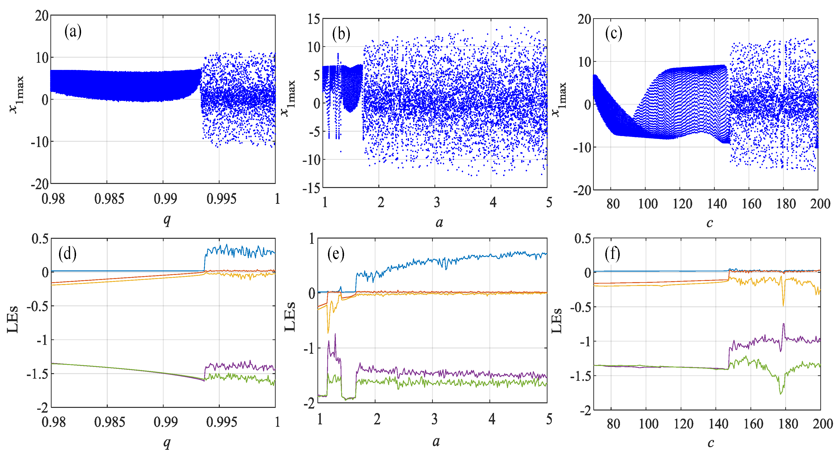
3.1. Bifurcation Analysis

To investigate the dynamics of system (2), three different cases are considered as follows. It is crucial to state here that the initial values of the system in these three cases are set as x 0 = [ 0.1 , 0.2 , 0.3 , 0.4 , 0.5 ] , and the sequence length is N = 10 4 with removing the first 10 4 points of data.
(1) Fix a = 2.0, b = 0.8, c = 70, d = 0.01, Q 1 = 0.005, Q 2 = 0.01 and vary q from 0.98 to 1 with a step size of 8 × 10 5 . Figure 2a,b depict the dynamics of system (2) using two significant analyses, which are the bifurcation diagram and Lyapunov exponents, respectively. Multi-periodic or periodic appears when q takes smaller values, but it becomes to be chaotic when q > 0.993 . As a result, with the derivative order, system (2) owns bright dynamics.
(2) Fix b = 0.8, c = 70, d = 0.01, Q 1 = 0.005, Q 2 = 0.01, q = 0.999 and vary a from 1 to 5 with a step size of 0.016 . Figure 2b,e shows that the system is totally chaotic with different values of parameter a, and the largest Lyapunov exponents increase with the growth of parameter a. It means that the complexity of the system increases with the growing values of a.
(3) Fix a = 2.0, c = 100, d = 0.01, Q 1 = 0.005, Q 2 = 0.01, q = 0.98 and vary c from 70 to 200 with a step size of 0.52. The dynamics of system (2) are depicted in Figure 2c,f. As shown in Figure 2c,f, the system becomes too chaotic when c > 148 . However, starting from q = 0.98 , the maximum Lyapunov exponent is close to zero.
According to the bifurcation diagram results in the above three cases, the system is chaotic with a relatively large derivative order q, the parameters a and c. Vary q from 0.95 to 1 with a step size of 5 × 10 4 , and vary a from 1 to 5 with a step size of 0.04 . The largest Lyapunov exponents contour plot of the system is illustrated in Figure 3a. Obviously, the system has relatively large Lyapunov exponents in the top right corner of the parameter plane. Meanwhile, the minimum order for chaos is about q = 0.96 according to Figure 3a. Moreover, we vary the derivative order 0.97 to 1 with a step size of 3 × 10 4 , and increase c from 70 to 200 with a step size of 1.3. The largest Lyapunov exponents contour plot is depicted in Figure 3b. It is clear that the higher complexity values of the system appear with larger values of q and the smaller values of c.

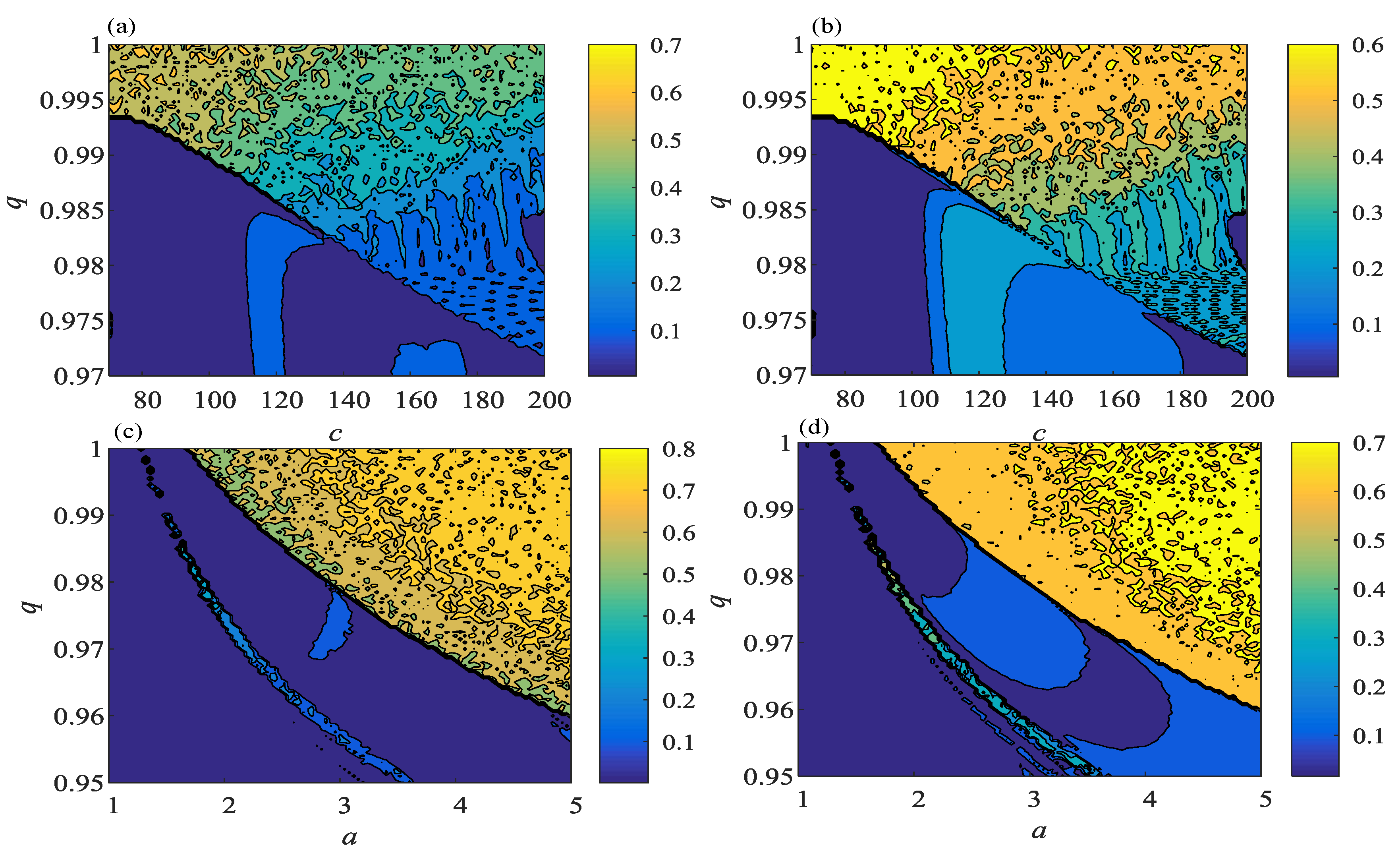
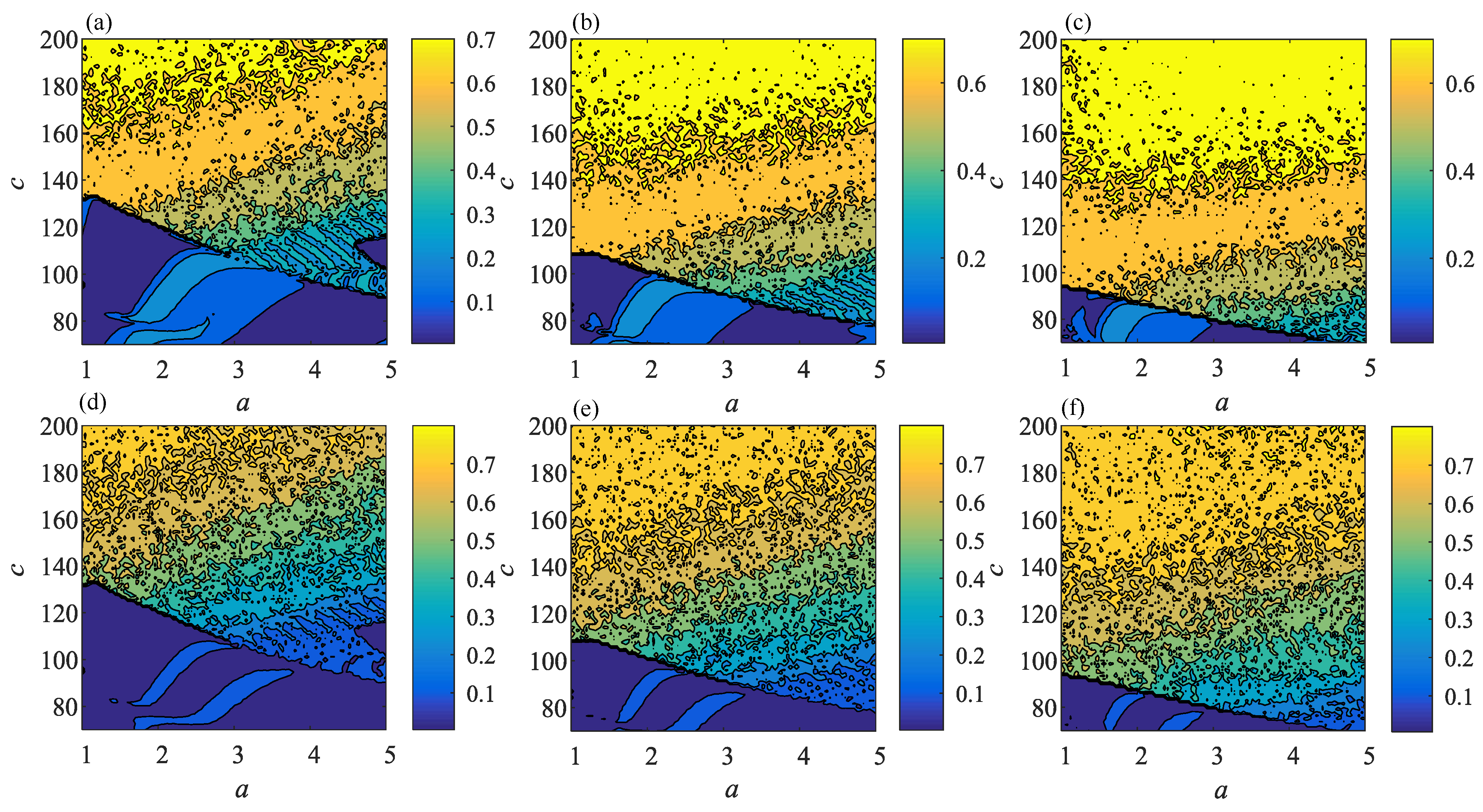
3.2. Multiscale Complexity Analysis

Suppose that the time series { x ( n ) , n = 0 , 1 , 2 , 3 , , N 1 } , and its corresponding discrete Fourier transformation is given by
X ( k ) = n = 0 N 1 x ( n ) e j 2 π N n k = n = 0 N 1 x ( n ) W N n k ,
where k = 0 , 1 , , N 1 and j = 1 is the imaginary unit. If the power of a discrete power spectrum with the kth frequency is | X ( k ) | 2 , then the probability of this frequency is defined as
P k = | X k | 2 k = 0 N / 2 1 | X k | 2 .
Using the discrete Fourier transformation, the summation runs from k = 0 to k = N / 2 1 . The entropy of this probability distribution with the same summation limits in Equation (8) is [17]
SE ( x ) = 1 ln ( N / 2 ) k = 0 N / 2 1 P k ln P k .
Assume the square value of { X ( k ) , k = 0 , 1 , 2 , , N 1 } is
G N = 1 N k = 0 N 1 | X ( k ) | 2 .
In addition, suppose
X ˜ ( k ) = X ( k ) i f | X ( k ) | 2 > ξ G N 0 i f | X ( k ) | 2 ξ G N ,
where ξ is a control parameter, then the C 0 complexity algorithm can be defined as [18]
C 0 ( x , r ) = k = 0 N 1 | X ( k ) X ˜ ( k ) | 2 n = 0 N 1 | X ( k ) | 2 .
Now, the consecutive coarse-graining of a one-dimensional discrete time series is given by [19]
y τ ( j ) = 1 τ ( j 1 ) τ j τ 1 x ( j ) ,
where 1 j [ N / τ ] , τ represents the non-overlapping window length. Distinctly, for  τ = 1 , the sequence y τ represents the prime sequence { x ( n ) , n = 0 , 1 , 2 , , N 1 } . However, the multiscale complexity in this paper is defined as [20]
MSE = 1 τ max τ = 1 τ max SE ( y τ ) ,
and
M C 0 = 1 τ max τ = 1 τ max C 0 ( y τ ) .
MSE and MC 0 are employed to estimate the complexity of system (2), where the maximum scale factor τ m a x = 25 . Complexity results with q varying are plotted in Figure 4a,d, and complexity results with a and c are plotted in Figure 4b–e and Figure 4c–f, respectively. Meanwhile, complexity results in the q a and q c parameter planes are shown in Figure 5. Firstly, it is obvious that the complexity results coincide with the bifurcation diagram and Lyapunov exponents. Secondly, it means that the system exhibits high complexity for real applications. Here, we vary a from 1 to 5 with a step size of 0.04, and increase c from 70 to 200 with a step size of 1.3. The complexity contour plots with q = 0.98, 0.99 and 0.999 are shown in Figure 6. It can be observed that the wider region of high complexity values appear when q takes larger values. Meanwhile, the system exhibits larger complexity values when parameter c is larger, and the system has wider range of high complexity when the parameter a is relatively larger. In conclusion, q, a, and c determines the complexity performance of the system.

4. Network Dynamics of the Fractional-Order Laser Systems

4.1. Building of the Laser Network

In this section, the coupled ring network of different identical fractional-order laser systems is proposed. The equations of the network are defined as
D t 0 q x i , 1 = a x i , 1 x i , 3 x i , 1 2 + x i , 2 2 Q 2 x i , 1 + Q 1 x i , 2 + κ 2 K j N o d e s x j , 1 x i , 1 , D t 0 q x i , 2 = a x i , 2 x i , 4 x i , 1 2 + x i , 2 2 Q 1 x i , 1 Q 2 x i , 2 , D t 0 q x i , 3 = x i , 3 d x i , 4 + c x i , 5 x i , 1 , D t 0 q x i , 4 = x i , 4 d x i , 3 + c x i , 5 x i , 2 , D t 0 q x i , 5 = b x i , 5 + x i , 1 x i , 3 + x i , 2 x i , 4 ,
where κ is the coupled strength, 2 K is the number of the nearby nodes, N o d e s contains the index of the nearby nodes, and there are N nodes ( i = 1 , 2 , , N ) in the network. In this paper, each node contains a fractional-order laser system. As a matter of fact, the node i is connected with its nearby 2 K nodes. Figure 7 shows the networks of 50 nodes with different values of K. When K = 1 , each node is connected with its two neighbors. The dynamics of this kind of network are investigated by He et al. [39] but with different systems. When K > 1 , there are more connections, and the network becomes more and more complicated with the increase of K.
To find all the connected nodes ( N o d e s ), Algorithm 1 is designed. The input of variables are i, K and N. Here, we have 1 i N , 2 K < N . For instance, when K = 1 , i = 1 and N = 50 , the nodes found are j = 50 and j = 2 , while if i = 10 , the nodes find are j = 9 and j = 11 . The output of the function is a matrix, thus nodes found for i = 1 is N o d e s = [ 50 , 2 ] . Then the equations can be programmed, realized using the found N o d e s , namely, j takes values from the matrix N o d e s .
Algorithm 1 Find the index of neighbors of node i, the function name is Find Nodes ( i , K , N ) .
Input:i, K, N
Output: N o d e s
if i + K N then
   N o d e 1 = i + 1 i + K ;
else
   N o d e 1 = [ i + 1 N , 1 K ( N i ) ] ;
end if
if i K > 0 then
   N o d e 2 = i + 1 i + K ;
else
   N o d e 2 = [ 1 i 1 , N K + i N ] ;
end if
N o d e s = [ N o d e 1 , N o d e 2 ]

4.2. Synchronization and Chimera States in the Network

According to the complexity results and phase diagrams, which have been shown in Figure 1, we choose the system parameters a = 2.0, b = 0.8, c = 70, d = 0.01, Q 1 = 0.005 and Q 2 = 0.05. When q = 0.98 , the system is periodic, while q = 0.998 , the system is chaotic. Meanwhile, the number of the nodes in the network is 500, namely, N = 500 . The initialization of network is set using random numbers. As a result, in the simulations, we choose it as x 0 = r a n d o m ( 5 N , 1 ) . Meanwhile, let us define the network error with respect to time as
E r r o r t = 1 N i = 2 N x i , 1 x i 1 , 1 + x N , 1 x 1 , 1 .
It shows the difference between different nodes. If E r r o r ( t ) 0 , the network is synchronized. Otherwise, there is no synchronization. Meanwhile, if there are coexisting zero and nonzero values, chimera states can be observed.
The dynamics of the network with different values of q and number of connections K are investigated. Figure 8 demonstrates the spatiotemporal patterns of the ring network of fractional-order laser systems with 500 nodes and couple strength κ = 5 . When q = 0.98 , the spatiotemporal patterns of the network are shown in Figure 8a–c, and the errors are shown in Figure 8d–f. Meanwhile, q = 0.998 , the simulation results are shown in Figure 8g–l. When K = 10 , the networks with q = 0.98 and 0.998 are not synchronized. However, when q = 0.98 and K takes larger values, the network is synchronized. Moreover, when q = 0.998 and K equals 50 and 100, it can be seen in Figure 8g–l that the spatiotemporal behaviors demonstrate the coherent and incoherent states, thus there are chimera states. As a result, when q = 0.998 and κ = 5 , there is no synchronization with different K. We fix q = 0.998 and K = 100 , the spatiotemporal patterns of the network are obtained after three simulations and the results are shown in Figure 9. Since the initial conditions of each experiment is different due to the randomness, it shows that the network is also sensitive to the initial values.
Let the coupling strength κ = 5 and derivative order q = 0.98 and 0.998, and vary the connection number K = 15, 55, 95, 125 and 155. Each experiment is carried out two times with different initial conditions, and the network errors with respect to time are shown in Figure 10a–d. It shows that the network can be synchronized when q = 0.98 and K > 15 . However, when q = 0.998 , it shows in Figure 10c,d that the network cannot be synchronized and non-stationary chimera states are observed, where the positions of coherent and incoherent oscillators vary in time. Fix the connection number K = 50 and derivative order q = 0.98 and 0.998, and the coupling strength κ is set as 5, 15, 25, 35 and 45. The analysis results are shown in Figure 10e–h. For each q, the experiments are carried two times and they are obtained with different initial conditions. Obviously, the network is synchronized when q = 0.98 and the chimera state is observed when q = 0.998 . Generally, larger coupling strength κ and more connections K cannot make the network synchronized.
Therefore, it can be concluded that the network is hard to be synchronized when the fractional-order laser system is chaotic ( q = 0.998 ). Furthermore, the network is synchronized with proper coupling strength and connection numbers when the laser system is periodic ( q = 0.98 ). Since each node contains a fractional-order laser system, the network is a fractional-order network, and its dynamics are determined by the derivative order q. Meanwhile, states of the network are determined by the initial conditions, and the chimera states are observed in the network. We hold the opinion that the laser network can have complex dynamical behaviors.

5. Discussion

For the neural process in nature, there are many potential applications regarding the chimera states. For instance, the bump states in the neural system localized regions of coherent oscillation surrounded by incoherence deduced the chimera states. Furthermore, various types of neuronal diseases, including schizophrenia, Parkinson’s disease, Alzheimer’s disease, and epileptic seizures connect to the sorting of co-existence of synchronization and desynchronization [40]. However, as far as we know, although the optical chimera state is not a new topic and it has already been reported [41,42], there are few reports on the chimera state of the fractional-order laser network. As a matter of fact, an optical chimera state was observed in the experiments and simulations, and it shows that the amplitude-phase coupling is necessary for the formation of the chimera states.
Here, the network investigated is a ring coupled network with limited numbered neighbor links. In real situations, the network can be with other structures. However, the analysis results can be concluded that the fractional-order laser network can have complex dynamics and even show chimera states. The main reason comes from the complex dynamics of the laser system the amplitude-phase coupling. When the original laser system is chaotic, chimera states are observed. Otherwise, when the original laser system is periodic, the network can be synchronized.
However, we still hope there will be more experiments, which can point out the existence of fractional-order laser systems or can better explain the physical significance. Meanwhile, the existence of chimera states in the laser is observed. However, applications of chimera states in the laser system should be further investigated.

6. Conclusions

This paper has explored the complexity and synchronization of a fractional-order laser system. Multiscale SE and C 0 algorithms have been applied to analyze the complexity performance of the time series of the system. Meanwhile, the ring network of the fractional-order laser models has been built with the presence of periodic and chaotic states. The following conclusions are stressed.
(1) Symmetric chaotic attractors and periodic circuits are observed, and chaos is found in the system.
(2) It can be observed that the fractional-order laser system has a wide range of high complexity regions in the parameter planes.
(3) It exhibits rich dynamics with the variance of q, a, and c, which was verified by a bifurcation diagram, phase diagram, MSE complexity and MC 0 complexity.
(4) Simulation results show that the chimera states can be observed only when the laser systems exhibit chaotic behaviors. Meanwhile, the network is synchronized with the periodic behaviors of the systems.
In fact, our analysis has demonstrated the complex behaviors of the proposed fractional-order laser network, especially the existence of different kinds of chimera states. Our next work will focus on the applications of chimera states in the fractional-order laser network.

Author Contributions

Conceptualization, S.B. and S.H.; methodology, H.N. and K.S.; software, S.H.; validation, S.H. and S.B.; formal analysis, S.B.; investigation, H.N. and S.H.; resources, H.N.; data curation, H.N.; writing—original draft preparation, S.H. and H.N.; writing—review and editing, S.B.; visualization, S.H.; supervision, S.B.; project administration, K.S.; funding acquisition, S.H. All authors have read and agreed to the published version of the manuscript.

Funding

Shaobo He was supported by the National Natural Science Foundation of China (Grant Nos. 61901530 and 62071496), the National Natural Science Foundation of Hunan Province, PR China (No. 2020JJ5767).

Institutional Review Board Statement

Not applicable.

Informed Consent Statement

Not applicable.

Data Availability Statement

All datasets generated for this study are included in the article.

Acknowledgments

The authors would like to thank the four anonymous reviewers for their constructive comments and insightful suggestions.

Conflicts of Interest

The authors declare no conflict of interest.

References

  1. Ichise, M.; Nagayanagi, Y.; Kojima, T. An analog simulation of non-integer order transfer functions for analysis of electrode processes. J. Electroanal. Chem. Interfacial Electrochem. 1971, 33, 253–265. [Google Scholar] [CrossRef]
  2. Tavazoei, M.S.; Mohammad, H. A proof for non existence of periodic solutions in time invariant fractional order systems. Automatica 2009, 45, 1886–1890. [Google Scholar] [CrossRef]
  3. Sun, H.; Zhang, Y.; Baleanu, D.; Chen, W.; Chen, Y. A new collection of real world applications of fractional calculus in science and engineering. Commun. Nonlinear Sci. Numer. Simul. 2018, 64, 213–231. [Google Scholar] [CrossRef]
  4. Su, D.; Bao, W.; Liu, J.; Gong, C. An efficient simulation of the fractional chaotic system and its synchronization. J. Frankl. Inst. 2018, 355, 9072–9084. [Google Scholar] [CrossRef]
  5. Pano-Azucena, A.D.; Tlelo-Cuautle, E.; Muñoz-Pacheco, J.M.; de la Fraga, L.G. FPGA-based implementation of different families of fractional-order chaotic oscillators applying Grünwald–Letnikov method. Commun. Nonlinear Sci. Numer. Simul. 2019, 72, 516–527. [Google Scholar] [CrossRef]
  6. He, S.; Santo, B. Epidemic outbreaks and its control using a fractional order model with seasonality and stochastic infection. Phys. Stat. Mech. Its Appl. 2018, 501, 408–417. [Google Scholar] [CrossRef]
  7. Lin, H.; Matthew, M.V.; Yu, Z. Synchronization of chaotic outputs in multi-transverse-mode vertical-cavity surface-emitting lasers. Opt. Commun. 2013, 309, 242–246. [Google Scholar] [CrossRef]
  8. Arroyo-Almanza, D.A.; Pisarchik, A.N.; Fischer, I.; Mirasso, C.R.; Soriano, M.C. Spectral properties and synchronization scenarios of two mutually delay-coupled semiconductor lasers. Opt. Commun. 2013, 301, 67–73. [Google Scholar] [CrossRef]
  9. Gottwald, G.A.; Ian, M. On the implementation of the 0–1 test for chaos. SIAM J. Appl. Dyn. Syst. 2009, 8, 129–145. [Google Scholar] [CrossRef]
  10. Rondoni, L.; Ariffin, M.R.K.; Varatharajoo, R.; Mukherjee, S.; Palit, S.K.; Banerjee, S. Optical complexity in external cavity semiconductor laser. Opt. Commun. 2017, 387, 257–266. [Google Scholar] [CrossRef]
  11. Natiq, H.; Said, M.R.M.; Ariffin, M.R.K.; He, S.; Rondoni, L.; Banerjee, S. Self-excited and hidden attractors in a novel chaotic system with complicated multistability. Eur. Phys. J. Plus 2018, 133, 1–12. [Google Scholar] [CrossRef]
  12. Natiq, H.; Banerjee, S.; Said, M.R.M. Cosine chaotification technique to enhance chaos and complexity of discrete systems. Eur. Phys. J. Spec. Top. 2019, 228, 185–194. [Google Scholar] [CrossRef]
  13. Natiq, H.; Kamel Ariffin, M.R.; Asbullah, M.A.; Mahad, Z.; Najah, M. Enhancing Chaos Complexity of a Plasma Model through Power Input with Desirable Random Features. Entropy 2021, 23, 48. [Google Scholar] [CrossRef]
  14. Bandt, C.; Bernd, P. Permutation entropy: A natural complexity measure for time series. Phys. Rev. Lett. 2002, 88, 174102. [Google Scholar] [CrossRef]
  15. Chen, W.; Zhuang, J.; Yu, W.; Wang, Z. Measuring complexity using fuzzyen, apen, and sampen. Med Eng. Phys. 2009, 31, 61–68. [Google Scholar] [CrossRef]
  16. Larrondo, H.A.; González, C.M.; Martin, M.T.; Plastino, A.; Rosso, O.A. Intensive statistical complexity measure of pseudorandom number generators. Phys. Stat. Mech. Its Appl. 2005, 356, 133–138. [Google Scholar] [CrossRef]
  17. Staniczenko, P.P.; Lee, C.F.; Jones, N.S. Rapidly detecting disorder in rhythmic biological signals: A spectral entropy measure to identify cardiac arrhythmias. Phys. Rev. 2009, 79, 011915. [Google Scholar] [CrossRef]
  18. En-hua, S.; Zhi-jie, C.; Fan-ji, G. Mathematical foundation of a new complexity measure. Appl. Math. Mech. 2005, 26, 1188–1196. [Google Scholar] [CrossRef]
  19. Costa, M.; Goldberger, A.L.; Peng, C.-K. Multiscale entropy analysis of biological signals. Phys. Rev. 2005, 71, 021906. [Google Scholar] [CrossRef] [Green Version]
  20. He, S.; Kehui, S.; Huihai, W. Complexity analysis and DSP implementation of the fractional-order Lorenz hyperchaotic system. Entropy 2015, 17, 8299–8311. [Google Scholar] [CrossRef] [Green Version]
  21. Boccaletti, S.; Latora, V.; Moreno, Y.; Chavez, M.; Hwang, D.U. Complex networks: Structure and dynamics. Phys. Rep. 2006, 424, 175–308. [Google Scholar] [CrossRef]
  22. Hai, X.; Ren, G.; Yu, Y.; Xu, C.; Zeng, Y. Pinning synchronization of fractional and impulsive complex networks via event-triggered strategy. Commun. Nonlinear Sci. Numer. Simul. 2020, 82, 105017. [Google Scholar] [CrossRef]
  23. Sheikholeslami, M.; Gerdroodbary, M.B.; Moradi, R.; Shafee, A.; Li, Z. Application of Neural Network for estimation of heat transfer treatment of Al2O3-H2O nanofluid through a channel. Comput. Methods Appl. Mech. Eng. 2019, 344, 1–12. [Google Scholar] [CrossRef]
  24. Majhi, S.; Bera, B.K.; Ghosh, D.; Perc, M. Chimera states in neuronal networks: A review. Phys. Life Rev. 2019, 28, 100–121. [Google Scholar] [CrossRef]
  25. Wei, Z.; Parastesh, F.; Azarnoush, H.; Jafari, S.; Ghosh, D.; Perc, M.; Slavinec, M. Nonstationary chimeras in a neuronal network. EPL Europhys. Lett. 2018, 123, 48003. [Google Scholar] [CrossRef]
  26. Parastesh, F.; Jafari, S.; Azarnoush, H.; Hatef, B.; Namazi, H.; Dudkowski, D. Chimera in a network of memristor-based Hopfield neural network. Eur. Phys. J. Spec. Top. 2019, 228, 2023–2033. [Google Scholar] [CrossRef]
  27. Martens, E.A. Bistable chimera attractors on a triangular network of oscillator populations. Phys. Rev. E 2010, 82, 016216. [Google Scholar] [CrossRef] [Green Version]
  28. Abdel-Aty, A.H.; Khater, M.M.; Attia, R.A.; Abdel-Aty, M.; Eleuch, H. On the new explicit solutions of the fractional nonlinear space-time nuclear model. Fractals 2020, 28, 2040035. [Google Scholar] [CrossRef]
  29. Akbar, M.; Nawaz, R.; Ahsan, S.; Nisar, K.S.; Abdel-Aty, A.H.; Eleuch, H. New approach to approximate the solution for the system of fractional order Volterra integro-differential equations. Results Phys. 2020, 19, 103453. [Google Scholar] [CrossRef]
  30. Wu, G.Z.; Yu, L.J.; Wang, Y.Y. Fractional optical solitons of the space-time fractional nonlinear Schrodinger equation. Optik 2020, 207, 164405. [Google Scholar] [CrossRef]
  31. Lv, L.; Li, C.; Li, G.; Zhao, G. Cluster synchronization transmission of laser pattern signal in laser network with ring cavity. Sci. Sin. Phys. 2017, 47, 080501. [Google Scholar] [CrossRef]
  32. Şafak, K.; Xin, M.; Peng, M.Y.; Kärtner, F.X. Synchronous multi-color laser network with daily sub-femtosecond timing drift. Sci. Rep. 2018, 8, 11948. [Google Scholar] [CrossRef]
  33. Xiang, S.; Wen, A.; Pan, W. Synchronization Regime of Star-Type Laser Network With Heterogeneous Coupling Delays. IEEE Photonics Technol. Lett. 2016, 28, 1988–1991. [Google Scholar] [CrossRef]
  34. Ahmed, E.; Elgazzar, A.S. On fractional order differential equations model for nonlocal epidemics. Phys. A 2007, 379, 607–614. [Google Scholar] [CrossRef]
  35. Banerjee, S.; Mukhopadhyay, S.; Rondoni, L. Multi-image encryption based on synchronization of chaotic lasers and iris authentication. Opt. Lasers Eng. 2012, 50, 950–957. [Google Scholar] [CrossRef]
  36. Banerjee, S.; Saha, P.; Chowdhury, A.R. Chaotic aspects of lasers with host-induced nonlinearity and its control. Phys. Lett. A 2001, 291, 103–114. [Google Scholar] [CrossRef]
  37. Gorenflo, R. Fractional Calculus: Some Numerical Methods. Courses and Lectures-International Centre for Mechanical Sciences. 1997. Available online: http://www.fracalmo.org/download/rgcism10.pdf (accessed on 20 January 2021).
  38. Sun, H.H.; Abdelwahab, A.; Onaral, B. Linear approximation of transfer function with a pole of fractional power. IEEE Trans. Autom. Control. 1984, 29, 441–444. [Google Scholar] [CrossRef]
  39. He, S.; Sun, K.; Wang, H. Synchronisation of fractional-order time delayed chaotic systems with ring connection. Eur. Phys. J. Spec. Top. 2016, 225, 97–106. [Google Scholar] [CrossRef]
  40. Wang, Z.; Liu, Z. A Brief Review of Chimera State in Empirical Brain Networks. Front. Physiol. 2020, 11, 724. [Google Scholar] [CrossRef]
  41. Uy, C.H.; Weicker, L.; Rontani, D.; Sciamanna, M. Optical chimera in light polarization. APL Photonics 2019, 4, 056104. [Google Scholar] [CrossRef]
  42. Böhm, F.; Zakharova, A.; Schöll, E.; Lüdge, K. Amplitude-phase coupling drives chimera states in globally coupled laser networks. Phys. Rev. E 2015, 91, 040901. [Google Scholar] [CrossRef] [PubMed] [Green Version]
Figure 1. Phase portraits with a = 2 , b = 0.8 , c = 70 , d = 0.01 , Q 1 = 0.005 and Q 2 = 0.01 : (a) q = 0.98 ; (b) q = 0.998 .
Symmetry 13 00341 g001
Figure 2. Dynamics of the system (2): (ac) the bifurcation diagrams versus q, a, and c varying, respectively; (df) LEs versus q, a, c varying, respectively.
Symmetry 13 00341 g002
Figure 3. Maximum Lyapunov exponent based contour plots: (a) q a plane; (b) q c plane.
Symmetry 13 00341 g003
Figure 4. Complexity analysis results of the fractional-order laser system: (a) MSE with the derivative order q varying; (b) MSE with the parameter a varying; (c) MSE with the parameter c varying; (d) MC 0 with the derivative order q varying; (e) MC 0 with the parameter a varying; (f) MC 0 with the parameter c varying.
Symmetry 13 00341 g004
Figure 5. Complexity measure results based contour plots: (a) q c plane using MC 0 algorithm; (b) q c plane using MSE algorithm; (c) q a plane using MC 0 algorithm; (d) q a plane using MSE algorithm.
Symmetry 13 00341 g005
Figure 6. Complexity results based contour plots in a c plane: (a) MC 0 complexity with q = 0.98 ; (b) MC 0 complexity with q = 0.99 ; (c) MC 0 complexity with q = 0.999 ; (d) MSE complexity with q = 0.98 ; (e) MSE complexity with q = 0.99 ; (f) MSE complexity with q = 0.999 .
Symmetry 13 00341 g006
Figure 7. Examples of the proposed networks with 50 nodes: (a) K = 1 ; (b) K = 2 ; (c) K = 5 ; (d K = 15 .
Symmetry 13 00341 g007
Figure 8. Spatiotemporal patterns and errors of the ring network of fractional-order laser systems with 500 nodes and the couple strength κ = 5 : (ac) Spatiotemporal patterns with q = 0.98 and K equal to 10, 50, 100, respectively; (df) errors with q = 0.98 and K equal to 10, 50, 100, respectively; (gi) spatiotemporal patterns with q = 0.998 and K equal to 10, 50, 100, respectively; (jl) errors with q = 0.998 and K equal to 10, 50, 100, respectively.
Symmetry 13 00341 g008
Figure 9. Spatiotemporal patterns of the ring network of fractional-order laser systems with 500 nodes, the couple strength κ = 5 , the derivative order q = 0.998 and the connections number K = 100 : (a) the first time; (b) the second time; (c) the third time.
Symmetry 13 00341 g009
Figure 10. Errors of the ring network of fractional-order laser systems with 500 nodes: (a) κ = 5 , q = 0.98 , different K and the experiment of the first time; (b) κ = 5 , q = 0.98 , different K and the experiment of the second time; (c) κ = 5 , q = 0.998 , different K and the experiment of the first time; (d) κ = 5 , q = 0.998 , different K and the experiment of the second time; (e) K = 50 , q = 0.98 , different κ and the experiment of the first time; (f) K = 50 , q = 0.98 , different κ and the experiment of the second time; (g) K = 50 , q = 0.998 , different κ and the experiment of the first time; (h) K = 50 , q = 0.998 , different κ and the experiment of the second time.
Symmetry 13 00341 g010
Publisher’s Note: MDPI stays neutral with regard to jurisdictional claims in published maps and institutional affiliations.

