A Heuristic Approach to Shelf Space Allocation Decision Support Including Facings, Capping, and Nesting

Abstract

Shelf space on which products are exhibited is a scarce resource in the retail environment. Retailers regularly make decisions related to allocating products to their outlets’ limited shelf space. The aim of the paper was to develop a practical shelf space allocation model offering the possibility of horizontal and vertical product grouping, representing an item (product) with facings, capping, and nesting, with the objective of maximizing the retailer’s profit. Because real category-management problems address a lot of retailer’s rules, we expanded the basic shelf space allocation model, using shelf constraints, product constraints, multi-shelves constraints, and category constraints. To solve the problem, we proposed two adjustable methods that allowed us to achieve good results within a short time interval. The validity of algorithms was estimated, using the CPLEX solver and illustrated with example problems. Experiments were performed on data generated on the basis of real retail values. To estimate the performance of the proposed approach, 45 cases were tested. Among them, the proposed approach found solutions in 34 cases, while CPLEX found solutions only in 23 cases. The profit ratio of the proposed approach is, on average, 94.57%, with minimal and maximal values of 86.80% and 99.84%, accordingly.

1. Introduction

Shelf space is one of the most expensive resources in retail. Retailers regularly make decisions related to the allocation of products to their outlets’ limited shelf space. Increasing retailers’ profit by attracting customers’ attention and encouraging them to perform additional purchases can be implemented by proper category management in the retail store. Defining enough shelf space for a product and finding the best product position on planogram shelves are important issues with respect to shelf space allocation.

Appropriate shelf space allocation is one of the main factors to obtaining an edge in the very competitive retail industry [1]. Stores’ growing product ranges cause a great challenge for retailers. Many models allocating a large number of products to shelf space have been developed over recent years, with the goal to optimize the retailer’s objective under certain constraints and merchandising rules within the store.

The significance of store space allocation approaches and their importance for researchers and retailers in order to make correct decisions was highlighted by Yang and Chen [2]. Shelf space allocation decisions involve two steps: the amount of shelf space for a particular product category and the amount of shelf space for a particular product within each product category [3].

Many consumers decide on what to purchase already inside the store. They do not always prefer to choose the cheapest product from the range offered. Instead, a lot of factors, such as the perceived quality of the product, loyalty to a particular brand, brand reputation, appetite to try something new, and other marketing variables, impact their choice [3]. With appropriate merchandising tactics, the retailer can try to obtain more profit from consumers when they visit the store.

As the shelf space allocation problem (SSAP) is, in many cases, NP-hard, specialized heuristics and metaheuristics should be used. Such algorithms allow one to attain a satisfactory near-optimal solution but still do not guarantee a globally optimal value [4]. Yang [5] developed a heuristic that extends an approach often applied to the knapsack problem in order to find the solution to the SSAP, considering the profit from a product unit as weight and weight taking order as the priority index in space planning. His algorithm consists of preparatory, allocation, and termination phases. Yang and Chen [2] classified shelf space management strategies, including dominance, adaptation, and passiveness, on the grounds of a questionnaire survey. Drèze et al. [6] proposed a model to measure the effect of the reallocation of a product on the shelf and the between the sales of individual brands inside the product category. Gajjar and Adil [7] developed some heuristics to solve the retail SSAP with a linear profit function. Reyes and Frazier [3] proposed nonlinear integer SSAP for grocery stores, considering the relationships between customer service factors and profitability. Frontoni et al. [8] proposed a heuristic approach to the planogram supply to find and count multiple facings of the same item of a product. Fadıloğlu et al. [9] prepared an optimization model that created an appropriate product shelf mix based on the store requirements, to maximize profit, that can be used by the retailers. Jajja [10] used a dynamic model to solve the SSAP in the retail shop. He also performed a sensitivity analysis for some variables in the model for various space allocation scenarios in stores. Hübner and Schaal [11] studied the demand effects and developed the retailer’s optimization model that takes into account stochastic, space-dependent, and vertical-shelf-positions-dependent demand. They proposed a solution for both cases, i.e., with cross-space elasticity and without it. Hübner and Schaal [12] included, in their model, the effects of replenishment and inventory costs. Valenzuela and Raghubir [13] claimed that the bottom shelves were dedicated to cheaper brands, while luxury brands should be located on the top shelves. Furthermore, Desrochers and Nelson [14] declared that consumers’ purchasing decisions depended on the correct categorization into product families that specified associations between products and the visual display on the shelf.

Table 1. Overview of literature on solution approaches. Abbreviations used in the table are as follows: EA—exact approach; BB—branch-and-bound; DP—dynamic programming; H—heuristics; GA—genetic algorithm; SA—simulated annealing; TS—tabu search; VNS—variable neighborhood search; SW—squeaky wheel; ABC—artificial bee colony; PSO—particle swarm optimization; GRA—gradient approach; ●—author’s solution approach.

Author	Year	EA	BB	DP	H	GA	SA	TS	VNS	SW	ABC	PSO	GRA
Anderson and Amato [15]	1974	●
Hansen and Heinsbroek [16]	1979				●
Corstjens and Doyle [17]	1981		●
Zufryden [18]	1986			●
Bultez and Naert [19]	1989				●
Borin, Farris, and Freeland [20]	1994						●
Borin and Farris [21]	1995				●		●
Urban [22]	1998				●	●							●
Li and Tsai [23]	2001				●
Moholkar and Sanjeev [24]	2001					●
Rajaram and Tang [25]	2001				●
Yang [5]	2001				●
Rodrigues, Lim, and Qian [26]	2002				●					●
Lim, Rodrigues, and Zhang [1]	2004				●			●		●
Bai and Kendall [27]	2005				●		●
Hwang, Choi, and Lee [28]	2005					●							●
Esparcia-Alcazar, Lluch-Revert, Sharman, Albarracin-Guillem, and Palmer-Gato [29]	2006a					●
Esparcia-Alćazar, Lluch-Revert, Sharman, Albarracín-Guillem, and Palmer-Gato [30]	2006b					●
Kok and Fisher [31]	2007				●
Abbott and Palekar [32]	2008				●
Bai and Kendall [33]	2008												●
Esparcia-Alcázar and Martínez-García [34]	2008					●
Van Nierop and Fok [35]	2008						●
Hwang, Choi and Lee [36]	2009					●
Silva, Marikar, and Le [37]	2009				●
Gajjar and Adil [38]	2010				●
Hansen, Raut, and Swami [39]	2010				●	●
Hall, Kopalle, and Krishna [40]	2010			●
Murray, Talukdar, and Gosavi [41]	2010				●
Russell and Urban [42]	2010				●
Gajjar and Adil [7]	2011				●
Ozcan and Esnaf [43]	2011										●	●
Yapicioglu and Smith [44]	2012							●
Aloysius and Binu [45]	2013				●
Bai and Kendall [46]	2013						●						●
Pinto and Soares [47]	2013					●
Castelli and Vanneschi [48]	2014					●			●
Chen, Chiu, and Yang [49]	2014					●
Erol, Bulkan, and Agaoglu [50]	2015						●
Geismar, Dawande, Murthi, and Sriskandarajah [51]	2015				●
Pinto, Soares, Brazdil, Bravo, Davison, Jofré, Maldonado, and Weber [52]	2015					●	●					●
Bianchi-Aguiar, Silva, Guimarães, Carravilla, Oliveira, Amaral, Liz, and Lapela [53]	2016				●
Ghazavi and Lotfi [54]	2016	●				●
Ghoniem, Maddah, and Ibrahim [55]	2016				●
Hübner, Kuhn, and Kühn [56]	2016	●			●
Hübner and Schaal [57]	2016				●
Flamand, Ghoniem, Haouari, and Maddah [58]	2017				●
Heydari and Yousefli [59]	2017					●
Hübner and Schaal [11]	2017a				●
Hübner and Schaal [12]	2017b				●
Choubey [60]	2017					●
Rabbani, Salmanzadeh-Meydani, and Farshbaf-Geranmayeh [61]	2018					●
Düsterhöft, Hübner, and Schaal [62]	2020	●
Yu, Maglasang, and Tsao [63]	2020								●

provides an overview of approaches used to solve the SSAP.

In the previous research, only facings of product items were considered. Moreover, one of the key limitations in the literature is that it neglects merchandising rules based on the frequency of product moves and the product price. More precisely, it disregards the different vertical shelf levels based on product sales potentials. Missing is a model which simultaneously takes into account retailers’ location and practical pricing rules.

The objective of this article was to develop a practical retail shelf space allocation model with not only facings but also capping (i.e., placing a product on top of another one and rotating the top one) and nesting (placing a product inside another one, e.g., a basket or plate). The main contribution of the paper is the development of an SSAP model characterized by the following:

• Cap and nest parameters.
• Vertical and horizontal category rows by appropriate product grouping, which makes planograms visually attractive to customers; such an effect is very important in visual merchandising for retailers, who, in general, prefer to design their own display spaces on planograms.
• Associating products based on their sales potentials for properly locating them on the bottom or top shelves, as well as creating vertical product families and grouping them to make the planogram visually attractive.

We proposed a realistic SSAP model, considering four groups of constraints, namely shelf constraints, product constraints, multi-shelves constraints, and category constraints. We also developed a heuristic approach and performed experiments on various practical problem sizes, estimating the quality of the solution with the CPLEX solver. In our approach, we placed special emphasis on the possibility of its practical implementation by retail category managers, in order to deliver higher profits.

The remainder of the article is structured as follows. Section 2 describes the data and methods. Numerical results of the computational experiments are given in Section 3. Section 4 outlines the conclusion of our research.

2. Data and Methods

Retailers focus on efficiently arranging products on shelves, with the goal of maximizing profit margin/sales, improving customer satisfaction, and managing stock control. Planograms are graphic representations of products’ arrangement on shelves. With their help, retailers can define the position of a product and the number of its units. Besides the fact that the SSAP is only a small part on the whole set of the category management processes, it is an easy way to earn profits.

2.1. Variables and Parameters

In our research, we used the following variables and parameters. Subscripts indicate the variables’ indexes, and superscripts indicate the variables’ descriptions and should not be read as indexes. Parameters and indices are as follows:

• $K$—total number of categories.
• $G$—total number of subcategories.
• $S$—total number of shelves.
• $P$—total number of products.
• $k$—category index, $k=1,\dots ,K$.
• $g$—subcategory index,$g=1,\dots ,G$.
• $i$—shelf index, $i=1,\dots ,S$.
• $j$—product index, $j=1,\dots ,P$.

Category parameters are as follows:

• $m_k$—minimum category $k$ size per cent of the shelf length.
• $t_k$—maximum category size tolerance between shelves in category $k$.

Shelf parameters:

• $s_i^l$—length of the shelf $i$.
• $s_i^d$—depth of the shelf $i$.
• $s_i^h$—height of the shelf $i$.
• $s_i^b$—weight limit of the shelf $i$.

Product parameters:

• $p_j^w$—width of the product $j$.
• $p_j^d$—depth of the product $j$.
• $p_j^h$—height of the product $j$.
• $p_j^b$—weight of the product $j$.
• $p_j^s$—supply limit of the product $j$.
• $p_j^u$—unit profit of the product $j$.
• $p_j^k$—category of the product $j$.
• $p_j^g$—subcategory of the product $j$.
• $p_j^n$—nesting coefficient of the product $j$, $p_j^n<1$, or $p_j^n=0$ if the product cannot be nested.
• $p_j^{o_1}$—front orientation binary parameter.
• $p_j^{o_1}=\left\{\begin{array}{l}1, \mathrm{if} \mathrm{front} \mathrm{orientation} \mathrm{is} \mathrm{available} \mathrm{for} \mathrm{product} j\\ 0, \mathrm{otherwise}\end{array}\right\}$
• $p_j^{o_2}$—side orientation binary parameter.
• $p_j^{o_2}=\left\{\begin{array}{l}1, \mathrm{if} \mathrm{side} \mathrm{orientation} \mathrm{is} \mathrm{available} \mathrm{for} \mathrm{product} j\\ 0, \mathrm{otherwise}\end{array}\right\}$.
• $p_j^l$—cluster of the product $j$.
• $f_j^{\min }$—minimum number of facings of the product $j$.
• $f_j^{\max }$—maximum number of facings of the product $j$.
• $c_j^{\min }$—minimum number of caps per facings group of the product $j$.
• $c_j^{\max }$—maximum number of caps per facings group of the product $j$.
• $n_j^{\min }$—minimum number of nests of one facing of the product $j$.
• $n_j^{\max }$—maximum number of nests of one facing of the product $j$.
• $s_j^{\min }$—minimum number of shelves on which product $j$ can be allocated.
• $s_j^{\max }$—maximum number of shelves on which product $j$ can be allocated.

Decision variables are as follows:

• $x_{ij}=\left\{\begin{array}{l}1, \mathrm{if} \mathrm{product} j \mathrm{is} \mathrm{put} \mathrm{to} \mathrm{the} \mathrm{shelf} i\\ 0, \mathrm{otherwise}\end{array}\right\}$
• $f_{ij}$—number of facings of the product.
• $c_{ij}$—number of caps of the product.
• $n_{ij}$—number of nests of the product.
• $y_{ij}^{o_1}=\left\{\begin{array}{l}1, \mathrm{if} \mathrm{product} j \mathrm{is} \mathrm{put} \mathrm{to} \mathrm{the} \mathrm{shelf} i \mathrm{on} \mathrm{front} \mathrm{orientation} \\ 0, \mathrm{otherwise}\end{array}\right\}$.
• $y_{ij}^{o_2}=\left\{\begin{array}{l}1, \mathrm{if} \mathrm{product} j \mathrm{is} \mathrm{put} \mathrm{to} \mathrm{the} \mathrm{shelf} i \mathrm{on} \mathrm{side} \mathrm{orientation} \\ 0, \mathrm{otherwise}\end{array}\right\}$.

2.2. Problem Definition and Methods

The problem can be formulated as follows. The $P$, products, are assigned to a $K$, categories (product families), and $G$, subcategories (sales potentials), and then they are placed on $S$, shelves, on a planogram. The minimal space occupied by a category is defined on each planogram, which makes it visually attractive for customers. All categories are vertical, i.e., the products can be placed on all shelves. Obviously, products of the same category cannot be split by another vertical category. The sales potential subcategories are horizontal, i.e., products can be placed on the shelves with a greater or equal subcategory but cannot be placed on the shelf for a lower subcategory. This models the situation where more expensive products (with higher sales potentials) are located on the higher shelves (at eye level); cheaper products can be located on the lower shelves and on the higher ones. However, the overpriced brands cannot be located underneath. The problem is to find the optimal shelf space for each product category, $K$, defining the quantities of each product in order to maximize the retailers’ profit.

Table 2. Categories and sales-potential subcategory allocation rules. ●—product of the defined category and subcategory can be placed on a shelf of the defined category and subcategory. The higher sales-potential subcategory (10, 20, 30) is, the darker is the color. Different main colors (blue, green, red) represent different categories (A, B, C).

	Shelf Category	A			B			C
Product Category	Subcategory	10	20	30	10	20	30	10	20	30
A	10	●	●	●	●	●	●	●	●	●
	20		●	●		●	●		●	●
	30			●			●			●
B	10				●	●	●	●	●	●
	20					●	●		●	●
	30						●			●
C	10							●	●	●
	20								●	●
	30									●

explains the methods of allocating products on shelves based on a retailer’s rules. Products from category A and subcategory 10 can be placed on the shelves dedicated to categories A, B, and C, as well as subcategories 10, 20, and 30. Under other conditions, products from the category C and subcategory 30 cannot be placed on the shelves for other categories and subcategories. The next example represents B20, which can be placed on shelves B20, B30, C10, C20, and C30. Sales potentials are assigned with an initially selected step (in this case, it equals 10) because, in practice, if base product ranges are assigned to sales subcategories 10 and 20, but one seasonal or promotional shelf is included on the planogram only for a 2-week time shift, the retailer can easily assign seasonal or promotional products to sales potential 15, without reassigning the sales potentials of the base product range. Figure 1 and Figure 2 show category sizes on shelves with different sales potentials. The divisor which splits the categories may be flexible (Figure 1) or strict (Figure 2), which is steered by coefficient $m_k$ (the minimum category size is $m_k$, a percent of the shelf length) and coefficient $t_k$ (the maximum category size tolerance between shelves in the category, a percent of the shelf length). The idea for this is taken from practice: The category must exist on the planogram, the products in this category must be noticeable by customers, and beautiful vertical category rectangles should be built in categories.

The product can be placed on the shelf in a front orientation (width $p_j^w$ is taken as line parameter) or side orientation, at 90 degrees (depth $p_j^d$ is taken as width of the product). The products with the same characteristics, functions, or tastes can be grouped into clusters, to make a certain substitution effect and must be placed on the same shelf. This is done in an out-of-stock situation, when the customer can easily choose a similar product from another brand.

As in a real retail store, and depending on the product package’s physical characteristics, products can be capped, nested, or neither. Capping is product placement on top of one another, e.g., in the case of rectangular boxes, as with tea or sweets boxes. Nesting is product placement inside another one, as with bowls or plates.

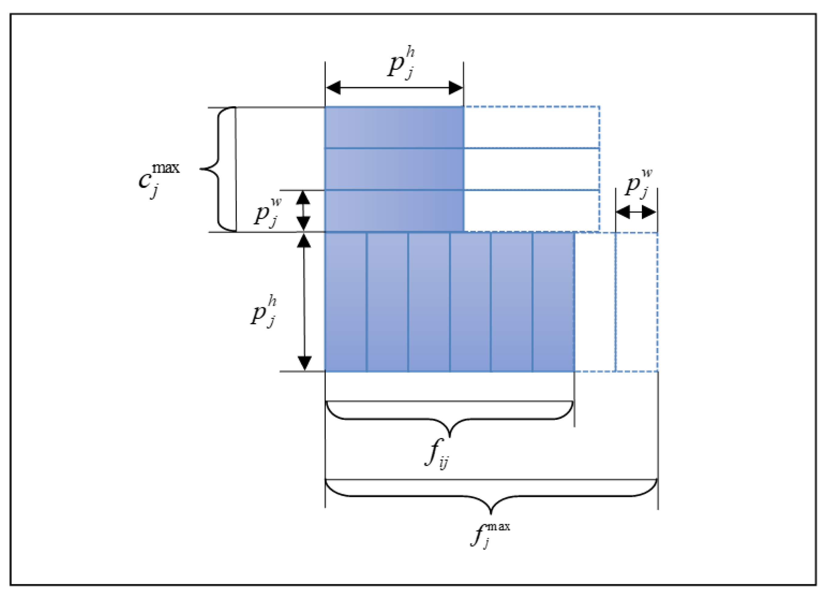
For products with a front orientation, the number of facings in one capped group is $\lceil p_j^h/p_j^w\rceil$, and for products with a secondary side orientation, it is $\lceil p_j^h/p_j^d\rceil$. For cappings, if too many tea boxes are placed above the facings in the row below, the boxes below may become damaged or destroyed, or upper tea boxes could fall off the shelf. For nestings, if too many bowls are placed inside the lowest bowl on the shelf, the bowl below may become damaged or destroyed, or the upper bowls could fall off the shelf. The total number of product items is the sum of facings, caps, and nests. Figure 3 and Figure 4 illustrate the caps and nests allocation method.

In our research, we considered one (top) row of facings with cappings or nestings on it. The number of facings in the vertical dimension is not modeled. The shelf height and product supply limit were defined only for the top row of facings, including capping or nesting. Similarly, the depth of the products and the depth of the shelf were defined for the same top row of facings.

To solve the problem, the task was to define the number of facings ($f_{ij}$), caps ($c_{ij}$), and nests ($n_{ij}$) of product $j$ placed on shelf $i$, with regard to constraints, which are grouped into 4 classes: shelf constraints, product constraints, multi-shelves constraints, and category constraints, in order to maximize the retailer’s total profit.

2.3. Basic Notions

2.3.1. Problem Formulation

The non-linear integer model can then be formulated as follows:

$$\max {\displaystyle \sum _{j=1}^P{\displaystyle \sum _{i=1}^S{x}_{ij}{p}_j^u(f_{ij}+c_{ij}+n_{ij})}}.$$

(1)

2.3.2. Shelf Constraints

The shelf constraints are as follows:

$$\forall (i)[{\displaystyle \sum _{j=1}^P{f}_{ij}(y_{ij}^{o_1}{p}_j^w+y_{ij}^{o_2}{p}_j^d)}\le s_i^l],$$

(2)

shelf length;

$$\begin{array}{l}\forall (i,j)[x_{ij}(p_j^h+\lceil \frac{c_{ij}{x}_{ij}}{\max (\lfloor \frac{f_{ij}(y_{ij}^{o_1}{p}_j^w+y_{ij}^{o_2}{p}_j^d)}{p_j^h}\rfloor ,1)}\rceil ·(y_{ij}^{o_1}{p}_j^w+y_{ij}^{o_2}{p}_j^d)+\\ +\lceil \frac{n_{ij}{x}_{ij}}{\max (f_{ij},1)}\rceil ·p_j^h{p}_j^n)\le s_i^h]\end{array},$$

(3)

shelf height;

$$\forall (i,j)[x_{ij}(y_{ij}^{o_1}{p}_j^d+y_{ij}^{o_2}{p}_j^w)\le s_i^d],$$

(4)

shelf depth;

$$\forall (i)[{\displaystyle \sum _{j=1}^P(f_{ij}+c_{ij}+n_{ij})p_j^b}\le s_i^b],$$

(5)

shelf weight.

Constraint (3) signifies that the height of each product on the shelf fit the shelf’s height limit. This was also true for the caps’ (Figure 3) height and nests’ height (Figure 4). As for the front-oriented products, their width represents the additional height to the product facings. Otherwise, as for the side-oriented products, their depth represents the additional height to the product facings. A construction such as $x_{ij}/\max (f_{ij},1)$ is used for omitting the division by 0 cases, i.e., if the product is not placed on the shelf.

2.3.3. Product Constraints

The product constraints are as follows:

$$\forall (j)[s_j^{\min }\le {\displaystyle \sum _{i=1}^S{x}_{ij}}\le s_j^{\max }],$$

(6)

minimum and maximum number of shelves;

$$\forall (j)[{\displaystyle \sum _{i=1}^S(f_{ij}}+c_{ij}+n_{ij})\le p_j^s],$$

(7)

supply limit;

$$\forall (j)[f_j^{\min }\le {\displaystyle \sum _{i=1}^S{f}_{ij}}\le f_j^{\max }],$$

(8)

minimum and maximum number of facings;

$$\forall (i,j)[c_j^{\min }\le c_{ij}\le c_j^{\max }·\lfloor \frac{f_{ij}(y_{ij}^{o_1}{p}_j^w+y_{ij}^{o_2}{p}_j^d)}{p_j^h}\rfloor ],$$

(9)

minimum and maximum number of caps;

$$\forall (i,j)[n_j^{\min }\le n_{ij}\le n_j^{\max }{f}_{ij}],$$

(10)

minimum and maximum number of nests;

$$\forall (i,j)[c_{ij}·n_{ij}=0],$$

(11)

either caps or nests.

2.3.4. Multi-Shelves Constraints

The multi-shelves constraints are as follows:

$$\forall (i,j)[y_{ij}^{o_1}·y_{ij}^{o_2}=0],$$

(12)

only one orientation (front or side) is available;

$$\forall (i,j)[y_{ij}^{o_1}+y_{ij}^{o_2}=1],$$

(13)

only one orientation (front or side) is available;

$$\forall (j)[\underset{i=1,\dots ,S}{\max }(y_{ij}^{o_1})\ne \underset{i=1,\dots ,S}{\max }(y_{ij}^{o_2})],$$

(14)

the same product orientation on all shelves;

$$\forall (i,j)[y_{ij}^{o_1}\le p_j^{o_1}],$$

(15)

front orientation is possible;

$$\forall (i,j)[y_{ij}^{o_2}\le p_j^{o_2}],$$

(16)

side orientation is possible;

$$\forall (j)\forall (a,b:\left|a-b\right|\ne 1\wedge a<b, a,b=1,\dots S)[x_{aj}·x_{bj}=0],$$

(17)

the next shelf only;

$$\forall (i)\forall (a,b: p_a^l =p_b^l, ? a,b=1,\dots P)[x_{ia}=x_{ib}],$$

(18)

the same cluster on the same shelf.

The same orientation on all shelves (Constraint (14)) is needed for building a better visual display of blocks on all shelves. For the same reason, products can be placed only on the neighboring shelf (Constraint (17)).

2.3.5. Category Constraints

The category constraints are a follows:

$$\forall (i,k)[{\displaystyle \sum _{\begin{array}{l}j=1,\\ p_j^k=k\end{array}}^P{f}_{ij}(y_{ij}^{o_1}{p}_j^w+y_{ij}^{o_2}{p}_j^d)}\ge \left[s_i^l·m_k\right]\vee {\displaystyle \sum _{\begin{array}{l}j=1,\\ p_j^k=k\end{array}}^P{f}_{ij}}=0],$$

(19)

minimum category size;

$$\begin{array}{l}\forall (k)[\underset{i=1,\dots ,S}{\max }({\displaystyle \sum _{\begin{array}{l}j=1,\\ p_j^k=k\end{array}}^P{f}_{ij}(y_{ij}^{o_1}{p}_j^w+y_{ij}^{o_2}{p}_j^d)})-\\ -\underset{i=1,\dots ,S}{\min }({\displaystyle \sum _{\begin{array}{l}j=1,\\ p_j^k=k\end{array}}^P{f}_{ij}(y_{ij}^{o_1}{p}_j^w+y_{ij}^{o_2}{p}_j^d)})\le \left[\underset{i=1,\dots ,S}{\max }(s_i^l)·t_k\right]]\end{array},$$

(20)

category tolerance between different shelves;

$$\forall (i,j)[x_{ij}\le \min (\max (s_i^g-p_j^g,0),1)],$$

(21)

sales potentials subcategory;

$$\left[\underset{i=1,\dots ,S}{\max }(s_i^l)·t_k\right]=\lfloor \underset{i=1,\dots ,S}{\max }(s_i^l)·t_k+0,5\rfloor ,$$

means rounded value.

Constraint (20) is used to form the border between neighboring categories on different shelves. Products with lower sales potentials, compared to the shelf, can be placed on shelves with greater sales potentials; otherwise, products with greater sales potentials, compared to the shelf, cannot be placed on the shelves with lower sales potentials (Constraint (21)).

2.3.6. Relationship Constraints

The relationship constraints are as follows:

$$\forall (i,j)[x_{ij}{s}_i^l(\frac{y_{ij}^{o_1}}{p_j^w}+\frac{y_{ij}^{o_2}}{p_j^d})\ge f_{ij}],$$

(22)

facings relationships;

$$\forall (i,j)[x_{ij}\le f_{ij}(y_{ij}^{o_1}+y_{ij}^{o_2})],$$

(23)

facings relationships;

$$\forall (i,j)[c_{ij}\le x_{ij}{c}_j^{\max }·\lfloor \frac{f_{ij}(y_{ij}^{o_1}{p}_j^w+y_{ij}^{o_2}{p}_j^d)}{p_j^h}\rfloor ],$$

(24)

capping relationships;

$$\forall (i,j)[n_{ij}\le x_{ij}{n}_j^{\max }{f}_{ij}],$$

(25)

nesting relationships.

2.3.7. Decision Variables

The decision variables are as follows:

$$x_{ij}\in \{0,1\},$$

(26)

product is placed on the shelf;

$$f_{ij}=\{f_j^{\min }\dots f_j^{\max }\},$$

(27)

number of facings;

$$c_{ij}=\{c_j^{\min }\dots c_j^{\max }·\lfloor \frac{f_{ij}(y_{ij}^{o_1}{p}_j^w+y_{ij}^{o_2}{p}_j^d)}{p_j^h}\rfloor \},$$

(28)

number of caps;

$$n_{ij}=\{n_j^{\min }\dots n_j^{\max }·f_j^{\max }\},$$

(29)

number of nests;

$$y_{ij}^{o_1}\in \{0,1\},$$

(30)

front orientation;

$$y_{ij}^{o_2}\in \{0,1\},$$

(31)

side orientation.

2.4. Proposed Approach

The main steps of the proposed approach include the following:

• Solve the decision problem in order to identify if the product can be placed on the shelf with regard to the multi-shelves constraints (Constraints (12)–(18)) and sales potentials subcategory Constraint (21). During this step, we set all possible products for shelf allocations.
• Select from the received set only allocations where number LB of product items fit shelf ((2)–(5)) and product ((6)–(11)) constraints.
• Solve the optimization problem (1) with regard to shelf Constraints (2)–(5), product Constraints (6)–(11), and category Constraints (19) and (20).

In this section, the following notations are used:

$\alpha$—integer coefficient of dividing shelf length into a number of product widths.

$\beta$—percent of solutions to be taken to the next steps of the algorithm.

The proposed algorithm of Step 3 is executed as follows. For the given shelf length, $s_i^l$, define all possible variations of line segments divisible by the product width, $\alpha p_j^w$ (or depth, $\alpha p_j^d$, based on its orientation). Integer coefficient $\alpha$ is selected empirically, i.e., the greater shelf length, the greater $\alpha$. Assign an appropriate number of facings, caps, and nests into the line segments for the given product. Thus, a number of possible solutions emerge. Apply this to all shelves in all categories. Exclude results where shelf ((2)–(5)), product ((6)–(11)), and category (19)–(20) constraints do not fit. Calculate the profit of each received solution. Apply Algorithm 1 and Algorithm 2 to the received solution set.

Algorithm 1 Steps

$\mathrm{Group} \mathrm{all} \mathrm{solutions} \mathrm{by} \mathrm{profit} {\displaystyle \sum _{j=1}^P{\displaystyle \sum _{i=1}^S{p}_j^u(f_{ij}+c_{ij}+n_{ij}).}}$ $\mathrm{For} \mathrm{each} \mathrm{one}, \mathrm{take} \mathrm{only} \mathrm{that} \mathrm{with} \mathrm{minimum} \mathrm{occupied} \mathrm{space} {\displaystyle \sum _{j=1}^P{\displaystyle \sum _{i=1}^S{f}_{ij}(y_{ij}^{o_1}{p}_j^w+y_{ij}^{o_2}{p}_j^d).}}$ $\mathrm{Sort} \mathrm{them} \mathrm{in} \mathrm{a} \mathrm{non}-\mathrm{ascending} \mathrm{order} \mathrm{of} \mathrm{profit}-\mathrm{to}-\mathrm{width} \mathrm{ratio} \frac{{\displaystyle \sum _{i=1}^S{\displaystyle \sum _{j=1}^P{p}_j^u(f_{ij}+c_{ij}+n_{ij})}}}{{\displaystyle \sum _{i=1}^S{\displaystyle \sum _{j=1}^P{f}_{ij}(y_{ij}^{o_1}{p}_j^w+y_{ij}^{o_2}{p}_j^d)}}} \mathrm{and} \mathrm{take} \beta$, an appropriate percentage of them (if there are too many of them). Select the best one.

There are three possible cases.

• The solution is ${\displaystyle \sum _{j=1}^P{\displaystyle \sum _{i=1}^S{p}_j^u(f_{ij}+c_{ij}+n_{ij})}}>0$. In this case, decrease $\alpha$, so additional possible solutions appear. Analyze only branches that give a greater total profit than the one received with the previous $\alpha$. If there are too many solutions to be analyzed, create profit branches for each category. In this case, the solution is found; the profit for each separate category is also known. Analyze only branches with higher profit categories, in order to create new possible solutions, and use only them. Leave less profitable profit category branches; choose appropriate percentage of branches to be analyzed based on their number received and the time used for generating them.
• The solution has not been found, and all values have been analyzed, so ${\displaystyle \sum _{j=1}^P{\displaystyle \sum _{i=1}^S{p}_j^u(f_{ij}+c_{ij}+n_{ij})}}=0$. Further, decrease $\alpha$ and analyze extra possible solutions.
• Not all values are analyzed at the given time limit. The solution has not been found, so ${\displaystyle \sum _{j=1}^P{\displaystyle \sum _{i=1}^S{p}_j^u(f_{ij}+c_{ij}+n_{ij})}}=\infty$. In this case, increase $\alpha$ so less possible solutions to be checked are generated, and repeat Algorithm 1.

Repeat Algorithm 1 an appropriate number of times, adjusting $\alpha$ and $\beta$.

Algorithm 2 Steps

$\mathrm{Group} \mathrm{all} \mathrm{solutions} \mathrm{according} \mathrm{to} \mathrm{occupied} \mathrm{space} {\displaystyle \sum _{j=1}^P{\displaystyle \sum _{i=1}^S{f}_{ij}(y_{ij}^{o_1}{p}_j^w+y_{ij}^{o_2}{p}_j^d).}}$ $\mathrm{For} \mathrm{each} \mathrm{one}, \mathrm{take} \mathrm{only} \mathrm{that} \mathrm{with} \mathrm{maximum} \mathrm{profit} {\displaystyle \sum _{j=1}^P{\displaystyle \sum _{i=1}^S{p}_j^u(f_{ij}+c_{ij}+n_{ij}).}}$ $\mathrm{Sort} \mathrm{them} \mathrm{in} \mathrm{a} \mathrm{non}-\mathrm{descending} \mathrm{order} \mathrm{of} \mathrm{space} \mathrm{occupied} \mathrm{on} \mathrm{the} \mathrm{shelves} \mathrm{and} \mathrm{take} \beta$, an appropriate percentage of them (if there are too many of them). Select the best one.

There are also three possible cases. Actions to be performed on them are the same as in Algorithm 1. Repeat Algorithm 2 an appropriate number of times, adjusting $\alpha$ and $\beta$.

3. Results

The computation experiments evaluated the quality of the solutions of the proposed approach to solving the current SSAP. To examine the performance of the proposed algorithm, simulated test problems based on real data were solved.

We simulated nine stores, where planograms with the defined product sets had to be placed. As in a retail store, shelf widths vary in different stores, but retailers must allocate in each store the same set of products. We simulated five planogram widths with three shelves with different sales potentials. The widths of all shelves on the planogram were the same because this was the regular case in a real store. Very rarely did a situation occur where store obstructions or inconvenient parts of the shelf decreased the shelf width. The prepared nine product sets included 10, 15, 20, 25, 30, 35, 40, 45, and 50 products with different widths, weights, and heights. The shelves widths were 250, 375, 500, 625, and 750 cm. The numbers of vertical categories were two (for 10, 15, and 20 products), three (for 25 and 30 products), four (for 35 and 40 products), and five (for 45 and 50 products).

The computational experiments were implemented in Visual C# 2015 and MS SQL Server 2014. The optimal (or maximum feasible, in some cases) solution to compare with was found with IBM ILOG CPLEX Optimization Studio Version: 12.7.1.0.

The benefit of both proposed algorithms is the lack of randomly selected elements, so there is no requirement to run them several times. Moreover, the data on all steps are visible and understandable for retailers, so all initial parameters can be easily checked, and the coefficient parameters can also be simply approximated, while watching the data and the received results.

Table 3. Number of solutions found by the proposed algorithms, where it was a maximum feasible solution.

Solution is Maximum Feasible Solution	Algorithm 1	Algorithm2
Number of solutions	25	18

shows the number of solutions found by both algorithms, where the solution of the proposed approach was the maximum feasible solution. Algorithm 2 was better, finding the maximum feasible solution in 25 cases.

Table 4. Number of solutions found by the proposed algorithm and CPLEX solver.

Solution Exists	Algorithms	CPLEX
Number of solutions	34	23

compares the proposed approach to the CPLEX solver, which found the solution in 34 cases, while CPLEX did in only 23, and affirmed the necessity of our implementations.

In order to estimate the performance of the algorithm, the following notations are used:

$U_a$—the profit of the proposed algorithm (Formula (1)).

$U_o$—the profit of the CPLEX solution.

$U_a/U_o$—the profit ratio of the proposed algorithm to the optimal (or maximum feasible, in some cases) solution.

Table 5. Solution quality, compared to the CPLEX solver.

Products	Shelf Width	Profit Ratio	Solution Exists	Total Number of Product Allocations	Processed Number of Product Allocations
10	250	98.30%	Algorithm, CPLEX	1.58 × 106	1.58 × 106
	375	98.52%	Algorithm, CPLEX	9.55 × 106	1.35 × 103
	500	97.93%	Algorithm, CPLEX	2.51 × 107	2.16 × 103
	625	97.01%	Algorithm, CPLEX	3.10 × 107	2.22 × 103
	750	97.31%	Algorithm, CPLEX	2.76 × 107	2.05 × 103
15	250		Algorithm	1.76 × 106	1.76 × 106
	375		Algorithm	2.00 × 105	4.77 × 102
	500		Algorithm	7.99 × 105	7.99 × 105
	625		Algorithm	1.31 × 107	4.27 × 103
	750		Algorithm	1.90 × 107	5.57 × 103
20	250			0.00	0.00
	375	99.84%	Algorithm, CPLEX	7.97 × 107	1.56 × 104
	500	97.72%	Algorithm, CPLEX	2.05 × 107	2.05 × 107
	625	92.68%	Algorithm, CPLEX	8.25 × 106	8.25 × 106
	750	88.07%	Algorithm, CPLEX	457 × 105	4.60 × 102
25	250	97.95%	Algorithm, CPLEX	7.18 × 106	7.18 × 106
	375	98.77%	Algorithm, CPLEX	6.25 × 107	2.06 × 105
	500	89.58%	Algorithm, CPLEX	1.10 × 106	2.16 × 104
	625	89.16%	Algorithm, CPLEX	3.60 × 106	4.73 × 104
	750	93.60%	Algorithm, CPLEX	9.39 × 106	7.00 × 104
30	250			0.00	0.00
	375			0.00	0.00
	500			0.00	0.00
	625			0.00	0.00
	750			0.00	0.00
35	250			0.00	0.00
	375	97.34%	Algorithm, CPLEX	1.71 × 109	3.31 × 106
	500	86.80%	Algorithm, CPLEX	1.10 × 1010	3.89 × 104
	625	90.87%	Algorithm, CPLEX	3.14 × 1012	1.94 × 106
	750	93.09%	Algorithm, CPLEX	7.40 × 109	1.07 × 105
40	250			0.00	0.00
	375	97.40%	Algorithm, CPLEX	7.46 × 109	9.99 × 104
	500	91.30%	Algorithm, CPLEX	1.04 × 108	1.15 × 106
	625		Algorithm	3.52 × 1012	8.19×105
	750		Algorithm	2.74 × 1013	1.65×106
45	250			0.00	0.00
	375	87.87%	Algorithm, CPLEX	1.16 × 1012	1.16×107
	500	95.86%	Algorithm, CPLEX	6.30 × 107	6.30×107
	625		Algorithm	1.05 × 1010	7.00×103
	750	98.08%	Algorithm, CPLEX	3.42 × 1014	1.46×105
50	250			0.00	0.00
	375			0.00	0.00
	500		Algorithm	1.44 × 1013	1.20 × 106
	625		Algorithm	1.57 × 1014	1.75 × 106
	750		Algorithm	2.46 × 1013	1.72 × 106
Min		86.80%		0.00	0.00
Average		94.57%		1.28 × 1013	2.87 × 106
Max		99.84%		3.42 × 1014	6.30 × 107
Median		97.01%		1.31 × 107	4.73 × 104
SD		4.17%		5.56 × 1013	9.90×106

shows the quality of the proposed approach, compared to the CPLEX solver. The average profit ratio of the best algorithm was 94.57%, with its minimal and minimal and maximal values at 86.80% and 99.84%, respectively. It could be observed that there are some advantages of the proposed approach. In 11 cases, the proposed approach found the solution, but CPLEX did not. Moreover, no opposite situation occurred where CPLEX found the solution but the proposed approach did not. In 11 cases, a solution was not found at all.

This case simulated the situation in a real retail store, where retailers requested something that could not be implemented based on the provided constraints. General mistakes that often happened in the retailer’s requirements are as follows:

• Even if the decision problem was successfully solved and a product could be placed on the shelf, the lower bounds numbers of a product on the shelf exceeded the shelf length or weight.
• Even if the lower bounds numbers satisfied the shelf length and weight, there were too many products in the category to be placed in aesthetically pleasing columns, which restricted the category constraints. The proposed corrections divided them into the categories in another way and changed the minimum category size or category tolerance.
• Even if there were lower bounds of product number, shelf length, and weight fit, the sales potentials of the products were incorrect, so that, on one shelf, there were too many products, and there were too few on another. In this case, it would be better to move some products from the most numerous subcategory to another sales potential subcategory.

These errors are visible and could be analyzed while processing each instance. Therefore, there is no reason to waste time trying to find the solution by using data in which we know every solution step fails to satisfy initial constraints.

Table 5 also illustrates the total number of product allocations received when solving the product-on-shelf decision problem. The last column shows the reduced number of product allocations, which was enough to be processed according to the proposed solution approach. The main idea was that, at first, we estimated how many decisions existed, and for each, we adjusted the appropriate number of product facings, caps, and nests. If we had enough time, we processed all of the product allocations. If there were too many allocations to be processed and it could not be done in a reasonable time, we reduced the number of allocations to be processed and selected more profitable ones according to Algorithms 1 and 2. When solving the optimization problem, we did not check all permutations of facings either, because there were too many variants. We also used the idea of the proposed Algorithms 1 and 2, which generated only profitable variants.

Table 6. Time taken looking for the solution and the total processing time.

	Time Taken Looking for the Solution		Total Time
	Seconds	Minutes	Seconds	Minutes
Min	2	0.03	2	0.49
Average	323	5.39	434	9.53
Max	5039	83.98	5170	87.11
Median	98	1.64	215	5.43
SD	856	14.27	892	15.01

presents the processing time taken to look for the solution while solving the optimization problem by both algorithms, which, on average, amounts to 5.39 min and varies from 2 s up to 83.98 min. The total processing time includes all preparation steps and solves the decision problem. On average, it amounts to 9.53 min and varies from 2 s to 87.11 min. The time limit for the CPLEX solver was set as 15 min because it was much more than the average and median time of the algorithms, and the standard deviation was approximately 15 min. In most cases, both proposed approaches were faster.

4. Conclusions

Shelf space is one of the most important resources used to involve more customers in category management decisions.

In this article, we proposed a new practicable mathematical shelf space allocation model with regard to horizontal products grouped into categories and vertical shelf levels grouped into sales potentials subcategories. The model includes cap and nest parameters. We developed two heuristic approaches and explained, in detail, how to implement them during category management problems. We also offered suggestions to space planners, focusing on general mistakes in requirements and how they should be corrected.

To estimate the performance of the proposed approach, 45 cases were tested. Among them, the proposed approach found solutions in 34 cases, while CPLEX achieved it only in 23 cases. The profit ratio of the proposed approach was, on average, 94.57%, with its minimal and maximal values being 86.80% and 99.84%, respectively.

The main feature that differentiates the proposed approach from the previous ones was the lack of randomly generated or randomly adjusted elements. At first, we solved the decision problem in order to check if the product fit the shelf; next, we solved the optimization problem, finding the appropriate number of facings of each product. Moreover, the data at all described steps could be easily analyzed and allowed us to adjust the steering parameters.

The main disadvantages of the proposed approach are as follows. If the product width (or depth, based on its orientation) is very small, there are too many possible variations of line segments initially generated. In situations where there are too many variants to be checked and the solution is not found within the given time, it is recommended to increase $\alpha$, dividing the shelf into larger parts. This method can decrease the number of variants and decrease processing time, which worsens the solution quality by increasing the distance of the feasible solution that can be found to the optimal one.

Our approaches are valuable for retailers looking for expert advice on techniques that could be used to solve the SSAP, which would enable them to maximize profit, minimize lost revenue, and find a balance between ensuring customer satisfaction and dealing with multiple inputs.

References

1. Lim, A.; Rodrigues, B.; Zhang, X. Metaheuristics with Local Search Techniques for Retail Shelf-Space Optimization. Manag. Sci. 2004, 50, 117–131. [Google Scholar] [CrossRef]
2. Yang, M.H.; Chen, W.C. Study on shelf space allocation and management. Int. J. Prod. Econ. 1999, 60–61, 309–317. [Google Scholar] [CrossRef]
3. Reyes, P.M.; Frazier, G.V. Goal programming model for grocery shelf space allocation. Eur. J. Oper. Res. 2007, 181, 634–644. [Google Scholar] [CrossRef]
4. Hübner, A. Retail Category Management: Decision Support Systems for Assortment, Shelf Space, Inventory and Price Planning; Springer: Berlin/Heidelberg, Germany, 2011; Volume 656. [Google Scholar]
5. Yang, M.H. Efficient algorithm to allocate shelf space. Eur. J. Oper. Res. 2001, 131, 107–118. [Google Scholar] [CrossRef]
6. Drèze, X.; Hoch, S.J.; Purk, M.E. Shelf management and space elasticity. J. Retail. 1994, 70, 301–326. [Google Scholar] [CrossRef] [Green Version]
7. Gajjar, H.K.; Adil, G.K. Heuristics for retail shelf space allocation problem with linear profit function. Int. J. Retail Distrib. Manag. 2011, 29, 144–155. [Google Scholar] [CrossRef]
8. Frontoni, E.; Contigiani, M.; Ribighini, G. A heuristic approach to evaluate occurrences of products for the planogram maintenance. In Proceedings of the MESA 2014—10th IEEE/ASME International Conference on Mechatronic and Embedded Systems and Applications, Senigallia, Italy, 10–12 September 2014. [Google Scholar]
9. Fadiloglu, M.M.; Karaşan, O.E.; Pinar, M.Ç. A model and case study for efficient shelf usage and assortment analysis. Ann. Oper. Res. 2010, 180, 105–124. [Google Scholar] [CrossRef] [Green Version]
10. Jajja, M.S.S. Retail shelf space allocation analysis using system dynamics approach. J. Qual. Technol. Manag. 2013, 9, 99–129. [Google Scholar]
11. Hübner, A.; Schaal, K. A shelf-space optimization model when demand is stochastic and space-elastic. Omega 2017, 68, 139–154. [Google Scholar] [CrossRef]
12. Hübner, A.; Schaal, K. An integrated assortment and shelf-space optimization model with demand substitution and space-elasticity effects. Eur. J. Oper. Res. 2017, 261, 302–316. [Google Scholar] [CrossRef]
13. Valenzuela, A.; Raghubir, P. Center of Orientation: Effect of Vertical and Horizontal Shelf Space Product Position. ACR N. Am. Adv. 2009, 36, 100–103. [Google Scholar]
14. Desrochers, D.M.; Nelson, P. Adding consumer behavior insights to category management: Improving item placement decisions. J. Retail. 2006, 82, 357–365. [Google Scholar] [CrossRef]
15. Anderson, E.E.; Amato, H.N. Mathematical Model for Simultaneously Determining the Optimal Brand-Collection and Display-Area Allocation. Oper. Res. 1974, 22, 13–21. [Google Scholar] [CrossRef]
16. Hansen, P.; Heinsbroek, H. Product selection and space allocation in supermarkets. Eur. J. Oper. Res. 1979, 3, 474–484. [Google Scholar] [CrossRef]
17. Corstjens, M.; Doyle, P. A Model for Optimizing Retail Space Allocations. Manag. Sci. 1981, 27, 822–833. [Google Scholar] [CrossRef]
18. Zufryden, F.S. A dynamic programming approach for product selection and supermarket shelf-space allocation. J. Oper. Res. Soc. 1986, 37, 413–422. [Google Scholar] [CrossRef]
19. Bultez, A.; Gijbrechts, E.; Naert, P.; Abeele, P. Vanden Asymmetric cannibalism in retail assortments. J. Retail. 1989, 65, 153–192. [Google Scholar]
20. Borin, N.; Farris, P.W.; Freeland, J.R. A Model for Determining Retail Product Category Assortment and Shelf Space Allocation. Decis. Sci. 1994, 25, 359–384. [Google Scholar] [CrossRef]
21. Borin, N.; Farris, P. A sensitivity analysis of retailer shelf management models. J. Retail. 1995, 71, 153–171. [Google Scholar] [CrossRef] [Green Version]
22. Urban, T.L. An inventory-theoretic approach to product assortment and shelf-space allocation. J. Retail. 1998, 74, 15–35. [Google Scholar] [CrossRef]
23. Li, H.L.; Tsai, J.F. A fast algorithm for assortment optimization problems. Comput. Oper. Res. 2001, 28, 1245–1252. [Google Scholar] [CrossRef]
24. Moholkar, M.; Sanjeev, S. A Genetic Algorithm Based Approach to Unequal Capacity Scheduling in Complex Retail Environments. In Proceedings of the ORSI International Conference, Ahmedabad, India, 27–29 January 2001. [Google Scholar]
25. Rajaram, K.; Tang, C.S. The impact of product substitution on retail merchandising. Eur. J. Oper. Res. 2001, 135, 582–601. [Google Scholar] [CrossRef]
26. Rodrigues, B.; Lim, A.; Qian, Z. A Heuristic for Shelf Space Decision Support in the Retail Industry. In Proceedings of the American Conference on Information Systems AMCIS 2002 Proceedings, Dallas, TX, USA, 9–11 August 2002. [Google Scholar]
27. Bai, R.; Kendall, G. An investigation of automated planograms using a simulated annealing based hyper-heuristic. Oper. Res. Comput. Sci. Interfaces Ser. 2005, 32, 87–108. [Google Scholar]
28. Hwang, H.; Choi, B.; Lee, M.J. A model for shelf space allocation and inventory control considering location and inventory level effects on demand. Int. J. Prod. Econ. 2005, 97, 185–195. [Google Scholar] [CrossRef]
29. Esparcia-Alcazar, A.I.; Lluch-Revert, L.; Sharman, K.C.; Albarracin-Guillem, J.M.; Palmer-Gato, M.E. Towards an evolutionary tool for the allocation of supermarket shelf space. In Proceedings of the Eighth Annual Conference on Genetic and Evolutionary Computation, GECCO 2006, Proceedings, Seattle, WA, USA, 8–12 July 2006; pp. 1653–1660. [Google Scholar]
30. Esparcia-Alćazar, A.I.; Lluch-Revert, L.; Sharman, K.; Albarracín-Guillem, J.M.; Palmer-Gato, M.E. An Evolutionary Algorithm for the Product to Shelf Allocation Problem. In Proceedings of the IEEE Congress on Evolutionary Computation (CEC), Vancouver, BC, Canada, 16–21 July 2006; pp. 10966–10972. [Google Scholar]
31. Kök, A.G.; Fisher, M.L. Demand estimation and assortment optimization under substitution: Methodology and application. Oper. Res. 2007, 55, 1001–1021. [Google Scholar] [CrossRef]
32. Abbott, H.; Palekar, U.S. Retail replenishment models with display-space elastic demand. Eur. J. Oper. Res. 2008, 186, 586–607. [Google Scholar] [CrossRef]
33. Bai, R.; Kendall, G. A model for fresh produce shelf-space allocation and inventory management with freshness-condition-dependent demand. INFORMS J. Comput. 2008, 20, 78–85. [Google Scholar] [CrossRef]
34. Esparcia-Alcázar, A.I.; Martínez-García, A.I.; Albarracín-Guillem, J.M.; Palmer-Gato, M.E.; Merelo, J.J.; Sharman, K.C.; Alfaro-Cid, E. A multiobjective evolutionary algorithm for the linear shelf space allocation problem. In Lecture Notes in Computer Science (including subseries Lecture Notes in Artificial Intelligence and Lecture Notes in Bioinformatics); Springer: Berlin/Heidelberg, Germany, 2008. [Google Scholar] [CrossRef] [Green Version]
35. Van Nierop, E.; Fok, D.; Franses, P.H. Interaction between shelf layout and marketing effectiveness and its impact on optimizing shelf arrangements. Mark. Sci. 2008, 27, 1065–1082. [Google Scholar] [CrossRef] [Green Version]
36. Hwang, H.; Choi, B.; Lee, G. A genetic algorithm approach to an integrated problem of shelf space design and item allocation. Comput. Ind. Eng. 2009, 56, 809–820. [Google Scholar] [CrossRef]
37. Landa-Silva, D.; Marikar, F.; Le, K. Heuristic approach for automated shelf space allocation. In Proceedings of the ACM Symposium on Applied Computing (SAC), Honolulu, HI, USA, 9–12 March 2009; pp. 922–928. [Google Scholar]
38. Gajjar, H.K.; Adil, G.K. A piecewise linearization for retail shelf space allocation problem and a local search heuristic. Ann. Oper. Res. 2010, 179, 149–167. [Google Scholar] [CrossRef]
39. Hansen, J.M.; Raut, S.; Swami, S. Retail Shelf Allocation: A Comparative Analysis of Heuristic and Meta-Heuristic Approaches. J. Retail. 2010, 86, 94–105. [Google Scholar] [CrossRef]
40. Hall, J.M.; Kopalle, P.K.; Krishna, A. Retailer Dynamic Pricing and Ordering Decisions: Category Management versus Brand-by-Brand Approaches. J. Retail. 2010, 86, 172–183. [Google Scholar] [CrossRef]
41. Murray, C.C.; Talukdar, D.; Gosavi, A. Joint Optimization of Product Price, Display Orientation and Shelf-Space Allocation in Retail Category Management. J. Retail. 2010, 86, 125–136. [Google Scholar] [CrossRef]
42. Russell, R.A.; Urban, T.L. The location and allocation of products and product families on retail shelves. Ann. Oper. Res. 2010, 179, 131–147. [Google Scholar] [CrossRef]
43. Ozcan, T.; Esnaf, S. A heuristic approach based on artificial bee colony algorithm for retail shelf space optimization. In Proceedings of the2011 IEEE Congress on Evolutionary Computation (CEC), New Orleans, LA, USA, 5–8 June 2011; pp. 95–101. [Google Scholar]
44. Yapicioglu, H.; Smith, A.E. Retail space design considering revenue and adjacencies using a racetrack aisle network. IIE Trans. Inst. Ind. Eng. 2012, 44, 446–458. [Google Scholar] [CrossRef]
45. Aloysius, G.; Binu, D. An approach to products placement in supermarkets using PrefixSpan algorithm. J. King Saud Univ. Comput. Inf. Sci. 2013, 25, 77–87. [Google Scholar] [CrossRef] [Green Version]
46. Bai, R.; van Woensel, T.; Kendall, G.; Burke, E.K. A new model and a hyper-heuristic approach for two-dimensional shelf space allocation. 4OR 2013, 11, 31–55. [Google Scholar] [CrossRef]
47. Pinto, F.; Soares, C. Space allocation in the retail industry: A decision support system integrating evolutionary algorithms and regression models. In Joint European Conference on Machine Learning and Knowledge Discovery in Databases; Springer: Berlin/Heidelberg, Germany, 2013; pp. 531–546. [Google Scholar]
48. Castelli, M.; Vanneschi, L. Genetic algorithm with variable neighborhood search for the optimal allocation of goods in shop shelves. Oper. Res. Lett. 2014, 42, 355–360. [Google Scholar] [CrossRef]
49. Chen, Y.K.; Chiu, F.R.; Yang, C.J. An optimization model for product placement on product listing pages. Adv. Oper. Res. 2014. [Google Scholar] [CrossRef] [Green Version]
50. Erol, H.; Bulkan, S.; Agaoglu, M. A Heuristic Approach for Shelf Space Allocation Problem. J. Mil. Inf. Sci. 2015, 4. [Google Scholar] [CrossRef]
51. Geismar, H.N.; Dawande, M.; Murthi, B.P.S.; Sriskandarajah, C. Maximizing Revenue through Two-Dimensional Shelf-Space Allocation. Prod. Oper. Manag. 2015, 24, 1148–1163. [Google Scholar] [CrossRef]
52. Pinto, F.; Soares, C.; Brazdil, P. Combining regression models and metaheuristics to optimize space allocation in the retail industry. Intell. Data Anal. 2015, 19, 149–162. [Google Scholar] [CrossRef] [Green Version]
53. Bianchi-Aguiar, T.; Silva, E.; Guimarães, L.; Carravilla, M.A.; Oliveira, J.F.; Amaral, J.G.; Liz, J.; Lapela, S. Using analytics to enhance a food retailer’s shelf-space management. Interfaces 2016, 46, 424–444. [Google Scholar] [CrossRef] [Green Version]
54. Ghazavi, E.; Lotfi, M.M. Formulation of customers’ shopping path in shelf space planning: A simulation-optimization approach. Expert Syst. Appl. 2016, 55, 243–254. [Google Scholar] [CrossRef]
55. Ghoniem, A.; Maddah, B.; Ibrahim, A. Optimizing assortment and pricing of multiple retail categories with cross-selling. J. Glob. Optim. 2016, 66, 291–309. [Google Scholar] [CrossRef]
56. Hübner, A.; Kuhn, H.; Kühn, S. An efficient algorithm for capacitated assortment planning with stochastic demand and substitution. Eur. J. Oper. Res. 2016, 250, 505–520. [Google Scholar] [CrossRef]
57. Schaal, K.; Hübner, A. When does cross-space elasticity matter in shelf-space planning? A decision analytics approach. Omega 2018, 80, 135–152. [Google Scholar] [CrossRef]
58. Flamand, T.; Ghoniem, A.; Haouari, M.; Maddah, B. Integrated assortment planning and store-wide shelf space allocation: An optimization-based approach. Omega 2018, 81, 134–149. [Google Scholar] [CrossRef]
59. Heydari, M.; Yousefli, A. A new optimization model for market basket analysis with allocation considerations: A genetic algorithm solution approach. Manag. Mark. 2017, 12, 1–11. [Google Scholar] [CrossRef] [Green Version]
60. Choubey, N. Floor Layout Optimization Using Genetic Algorithm. Int. J. Curr. Res. 2017, 9, 53529–53533. [Google Scholar]
61. Rabbani, M.; Salmanzadeh-Meydani, N.; Farshbaf-Geranmayeh, A.; Fadakar-Gabalou, V. Profit maximizing through 3D shelf space allocation of 2D display orientation items with variable heights of the shelves. OPSEARCH 2018, 9, 53529–53533. [Google Scholar] [CrossRef]
62. Düsterhöft, T.; Hübner, A.; Schaal, K. A practical approach to the shelf-space allocation and replenishment problem with heterogeneously sized shelves. Eur. J. Oper. Res. 2020, 282, 252–266. [Google Scholar] [CrossRef]
63. Yu, V.F.; Maglasang, R.; Tsao, Y.C. A reduced variable neighborhood search-based hyperheuristic for the shelf space allocation problem. Comput. Ind. Eng. 2020, 143, 106420. [Google Scholar] [CrossRef]
Figure 1. Allocation of categories and sales-potential subcategories, with a flexible border between the vertical categories. The higher sales-potential subcategory (10, 20, 30) is, the darker is the color. Different main colors (blue, green, red) represent different categories (A, B, C).
Symmetry 13 00314 g001
Figure 2. Allocation of categories and sales-potential subcategories, with a strict border between the vertical categories. The higher sales-potential subcategory (10, 20, 30) is, the darker is the color. Different main colors (blue, green, red) represent different categories (A, B, C).
Symmetry 13 00314 g002
Figure 3. Caps allocation.
Symmetry 13 00314 g003
Figure 4. Nests allocation.
Symmetry 13 00314 g004