1. Introduction
The desire to consider a wide range of space-time scales in physical systems study leads to increased interest in multiscale modeling [
1,
2,
3,
4]. Discrete element methods (DEM) are a powerful tool in this direction. Typically, methods of this type describe objects as a set of closely packed interacting particles. The particles move according to classical dynamics laws, and their motion can be described by a system of ordinary differential equations. The application of DEM is possible at various scale levels. The potential for parallelization of computations inherent in this family of methods makes it possible to have a high spatial-temporal resolution by increasing the number of discrete elements. We should also note that the method has the property to eliminate the shortcomings of the continuum models, which is especially important when the medium’s continuity is violated. In the case of the right choice of particle interaction potential and careful parameter tuning, such an approach allows for simulating quite complex processes [
5,
6,
7].
The most common method of this class is the molecular dynamics method. The system is considered a set of interacting discrete elements (atoms, molecules), the dynamics of which is described by the laws of classical mechanics. In this case, the parameters of the interatomic potential can be identified from the data of ab initio (quantum mechanical) calculations. Such an approach at the current level of computer technology makes it possible to simulate the behavior of systems consisting of up to hundreds of millions of structural elements, which corresponds to the nanometer size range (up to 1 μm). The use of structural formations consisting of a large number of atoms or molecules as discrete elements makes it possible to reach the mesoscopic level of describing systems. The critical point here is the availability of information about the parameters of interaction between elements. The coarse-grained methods are based on a generalization of the molecular dynamics approach. Effective realizations have been proposed for various systems [
8,
9,
10,
11,
12,
13]. A comprehensive review of this class of methods can be found in [
14]. One of the first implementations of DEM, as applied to two-dimensional problems, is setting the interaction mechanism by placing two virtual springs (longitudinal and transverse) between the elements with their elasticity parameters. Thus, longitudinal and shear stresses in the material are set depending on deformations. In this case, the parameters of elasticity can be estimated from the macroscopic response of the material to characteristic influences. The method was implemented in the Particle Flow Code (PFC2D). Some effective approaches have been developed using a combination of discrete elements and continuum mechanics methods [
15,
16,
17,
18,
19]. In [
20,
21], the cohesive discrete element method was presented where a continuous medium is modeled by packed granular spheres, and cohesive interaction between the spheres is described with beam elements. Another concept is laid on the basis of cellular automata methods. This approach is based on the representation of materials as a set of elements (cellular automata) that change their state at discrete times depending on the state of the element and its neighbors at the previous time moment. The evolution of a system of automata is determined by the rules of transition between states, which gives an alternative to describing processes using differential equations. Movable cellular automata [
22] have the ability of elements to move in space, which makes it possible to apply the method to fracture mechanics problems.
In our previous paper [
23], a discrete element method was proposed that adapts information on the microstructure of a material. The proposed method’s main feature is a combination of discrete elements and associated atomic samples. For the atomic sample, the molecular dynamics simulation is carried out to determine element properties. The natural assumption is used that the tensors of stress and deformation are equal for the discrete element and its atomic sample. This enables us to organize the information transfer between the levels. Thus, no macroscopic material properties have to be known; all the necessary information can be obtained by atomic sample simulation. In [
23], the method has been validated for materials with embedded-atom interatomic potentials.
This paper presents a full cycle of multiscale discrete-element modeling applied to the analysis of materials with covalent bonds. The paper’s novelty lies in the fact that all stages of multiscale modeling, including discrete-element modeling [
23], are considered in relation to polycrystalline materials with Tersoff interatomic potential. The first step of multiscale modeling is fitting interatomic potential to quantum mechanical properties. It is conducted using the quasi-Newton limited-memory Broyden–Fletcher–Goldfarb–Shanno (L-BFGS) optimization method. Gradients of the loss function are extracted using automatic differentiation. The data obtained in this way (the interatomic potential parameters) make it possible to proceed to model at the mesoscopic level. A polycrystalline object is simulated using discrete elements with randomly oriented lattices. Differential equations describing dynamics on macro and micro levels are solved in a self-consistent manner. As a result, polycrystalline silicon’s elastic properties are obtained only using data extracted from quantum mechanical information.
2. Materials and Methods
The discrete element method considers an object as an ensemble of
n interacting particles (discrete elements). Particle motion is described in terms of classical dynamics by the system of ordinary differential equations:
Here,
is a mass the
i-th particle,
a position vector, and
a force acting on the
i-th particle. Typically, the force is equal to the sum of forces caused by the interaction with the surrounding particles:
where
is a force with which the
j-th particle acts on the
i-th particle,
.
In the present work, to integrate the system (1)–(2), we use the Verlet velocity method of the second-order accuracy. This numerical scheme is symplectic and rather effective in terms of accuracy and computational cost. According to the method, first, the coordinates of the particles are updated, then the forces acting on the particles are calculated, after which the new particle velocities are determined from the average acceleration values over the time interval:
Here, k is a time step number and is a time step value.
Note that since the algorithm contains an implicit element when calculating velocities (the velocities on a new time layer are calculated from the acceleration (force) on a new layer), it has a reasonable margin of stability.
In our multiscale method, we use differential Equations (1)–(2) at two scale levels—atomic level and macro-element level. At the atomic level, the discrete elements are atoms interacting with interatomic potential. At the macro-element level, the discrete elements are tetrahedrons interacting by their faces. The dynamics of macro-elements is determined by their vertex motion. The connection between the systems at different levels is based on deformation and stress tensors. Here, we use a natural assumption that the tensors are the same for macro-element and its atomic sample.
The first step of the multiscale approach is ab initio (quantum mechanical) modeling. Ab initio methods allow for studying various properties of different materials, only requiring knowledge about the atomic composition of studied materials. Since these methods are computationally very costly, it is hard to implement them for systems with linear sizes of more than a few nanometers. For our goal, it is principal that from the ab initio modeling, we can get the unit cell size, cohesion energy, bulk modulus, and elastic constants of the material. This information is used for the parametric identification of the interatomic potential to carry out molecular dynamics modeling. In the present work, we consider the Tersoff potential, which adequately reflects the specificity of covalent bonds. The details of the identification are considered later in the paper.
When moving to the next macroscopic level, we represent the object as a set of tetrahedral elements stiffly bound by their faces [
23]. With every discrete element, we associate an atomic sample (representative fragment of atomic structure). For materials with a crystalline structure, the atomic sample is a representative (in terms of determining element properties) fragment of crystalline lattice oriented in a certain direction.
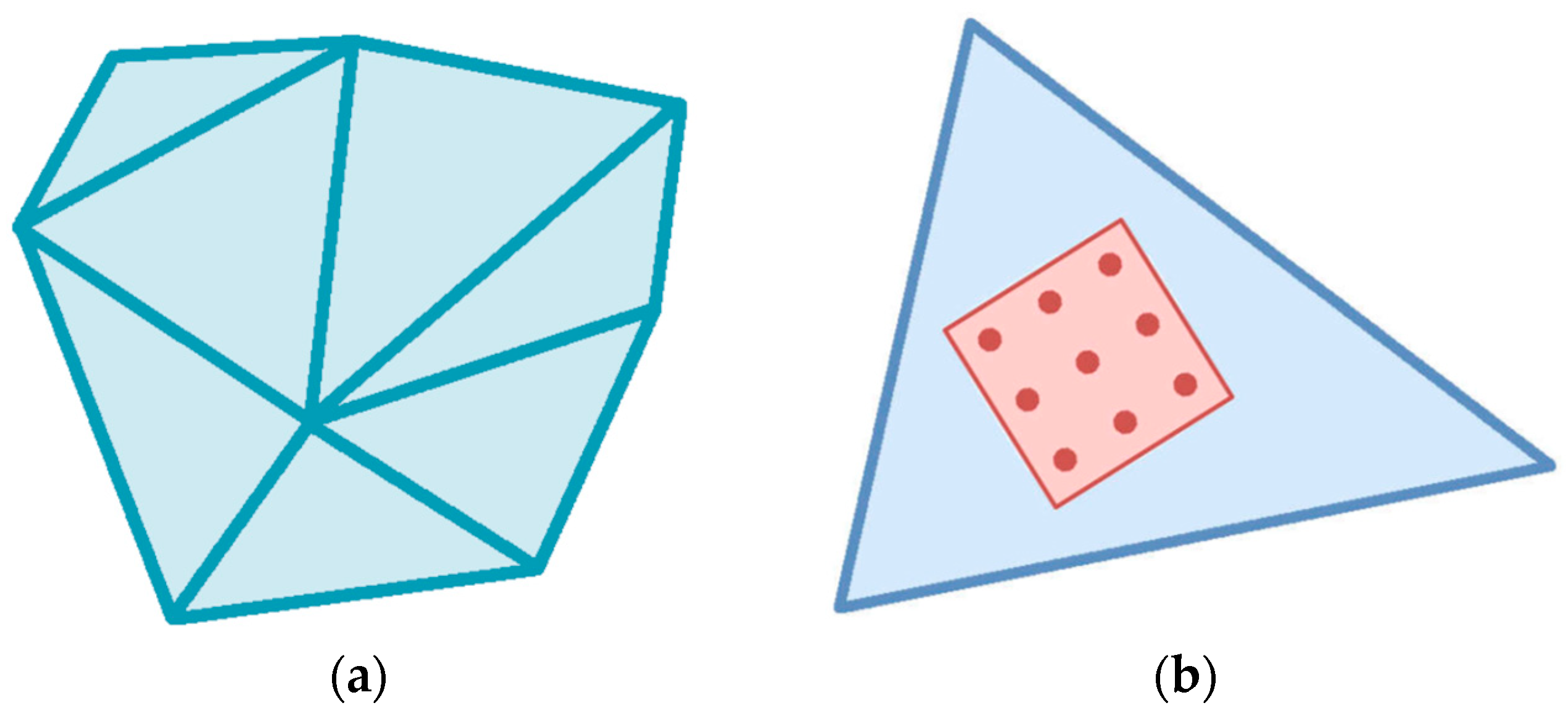
Figure 1 shows the object as a set of discrete macro-elements (
Figure 1a) and the atomic sample associated with the element (
Figure 1b).
Note that there is a huge difference in characteristic time and size between macroscopic discrete element (DE) and atomic sample (AS). Nevertheless, it is possible to organize the information transfer between the levels. A detailed description can be found in [
23]. We use a natural assumption that the tensors of stress and deformation are the same for the element DE and its atomic sample AS. Indeed, the AS associated with DE is a representative fragment of the element, and the DE volume is large enough not to take boundary effects into account. Thus, we can consider the DE properties to be entirely determined by the corresponding properties of the associated AS.
Here, we provide basic steps of self-consistent macro- and micro-dynamics.
Starting from macro-element deformation, we calculate the DE deformation tensor:
where
are initial position vectors of element vertexes and
are current position vectors of vertexes.
Assuming that the atomic sample associated with the element undergoes the same deformation as the element, we get the strain tensor for AS:
Having the deformation tensor, we can calculate new atom positions in the global coordinate system:
where
is the matrix of AS basis vectors so that the AS is a parallelepiped generated by these vectors,
is the lattice rotation matrix,
is the matrix of atomic positions in local fractional coordinates, and
N is the number of atoms in AS. The obtained positions are used on the next step as initial conditions.
Atomic dynamics is simulated solving the system of ordinary differential Equations (1)–(2) with numerical method (3). The system can be written in a matrix form:
where
is the diagonal matrix of atomic masses,
is the matrix of atomic velocities, and
is the potential energy function.
After the steady state is reached in the process of atomic dynamics simulation, we calculate the stress tensor of AS:
Here, is the AS volume and is the average atom velocity.
Assuming that the stress tensors of AS and DE are equal, we get the stress tensor for the element
Having the stress tensor
, we can calculate the forces acting on every vertex of the DE. Consider one face of the DE. The force
acting on the
k-th vertex (
k = 1,2,3) of the
m-th face of element
l is calculated using the force acting on the face
:
where
is the normal to face
m of element
l,
is the face area, and
is the part of face area attributed to vertex
. Similarly, we assign masses to vertices. We divide the element’s volume into four parts and distribute the element’s mass between the vertexes according to the corresponding volumes. Summation over all elements adjacent to the vertex gives the net force and effective mass of the vertex.
After forces acting on vertexes and vertex masses are determined, we calculate new vertex positions using the system of differential Equations (1)–(2) for vertex dynamics and numerical method (3).
Getting new vertex positions, we turn to step 1, and the computational process continues.
It should be noted that the proposed approach is computationally expensive. A three-dimensional model of an object requires a significant number of discrete elements, while for each element, it is necessary to get the relaxation of the associated atomic sample by molecular dynamics modeling. In this regard, the computations are parallelized on graphic processors. The computational process suits well the architecture of graphic processors since it consists of solving many not too large independent problems (molecular dynamics modeling inside each atomic sample).
3. Results and Discussion
In [
23], we validated the discrete element model on metals. Here, we consider a full cycle of multiscale modeling as applied to materials with covalent bonds. In this case, the interatomic interaction can be described with Tersoff potential, which adequately reflects the specificity of covalent bonds. The Tersoff potential was proposed in 1988, and it has been widely used in molecular dynamics [
24]. For a system of atoms of a single type, it can be written in the following form:
Here, rij is the distance between atoms i and j and θijk is the bond angle between the ij and ik bonds. This potential has 14 parameters, but R and D are always fixed before fitting so that atoms interact only with the nearest neighbors. Additionally, m is generally fixed and equal to 3, so effectively, there are only 11 parameters that can be used in the fitting.
As an example, we consider polycrystalline silicon, the characteristics of which are widely presented in the literature.
The potential parameters are identified to describe the elastic properties and cohesive energy of a material reasonably well. The target properties are cohesive energy (
Ec), bulk modulus (
B), elastic constants (
C′,
C11,
C12,
C440,
C44), and unit cell size (
a). Here,
C440 is the theoretical value obtained for
C44 in the absence of internal displacements. All target properties can be extracted from ab initio calculations; we do not dive into it but use some already known values.
Table 1 contains the values used [
25]. The unit cell size for a given parameter set is not directly computed, but instead, the loss function contains a derivative of the cell energy with respect to the cell size, which is required to be zero at the actual cell size so that the energy is minimized for the unit cell of appropriate size. All elastic properties are considered equally important so that the chosen loss function is a weighted root mean square error:
All elastic properties can be derived from the potential as a second derivative of the energy with respect to some deformation. For example, for
C440, the deformation matrix and resulting evaluation are as follows:
Here, Ω is the volume per atom. The required second derivatives can be evaluated numerically:
After fitting, several parameter sets with the lowest loss function are checked by molecular dynamics simulations for stability. A cube of 4 × 4 × 4 unit cells is modeled for 0.01 nanoseconds with four different boundary conditions: fully periodic in all directions, periodic in the x- and y-directions but not z-, periodic only in the x-direction, and non-periodic. The best stable parameters set is selected for further usage.
The optimization of the loss function is an important and rather complex problem. Methods of parametric identification of the Tersoff potential parameters are considered in [
26,
27]. One of the effective ways is using gradient methods based on automatic differentiation of loss function. In our work, the parameters are found using the L-BFGS algorithm, which requires the loss function gradient. Derivation of an analytical expression for the loss function gradient is a tedious and error-prone process, whereas the numerical evaluation of gradients using finite differences suffers from numerical inaccuracies. The automatic differentiation solves both of these problems; it is a technique for transforming an arbitrary program that calculates some numerical values of a function into a program that calculates numerical values of derivatives of that function with an accuracy close to that of a function evaluation [
28]. There are two main approaches to the implementation of automatic differentiation: forward and reverse accumulation. In general, for a function, f: Rn→Rm, reverse accumulation is preferable when
n >> m. Here, we use forward accumulation because the differentiation problem is rather modest, but for potentials with more parameters or multicomponent systems, reverse accumulation can be chosen. Automatic differentiation with forward accumulation can be implemented using the augmented algebra of real numbers. Each computation result is replaced by a pair of numbers: the result itself and its derivatives’ vector with respect to every variable. Then, every operation on such a pair is implemented in a way to keep the values and derivatives consistent.
It has to be noted that the L-BFGS algorithm is able to find a local minimum of the loss function, whereas the problem under consideration is multi-extremal. To solve this problem, the search is performed multiple times from different random start points.
The results of the identification are presented in
Table 1 and
Table 2. The target and calculated properties are given in
Table 1; the identified parameter set (the result of optimization) is shown in
Table 2.
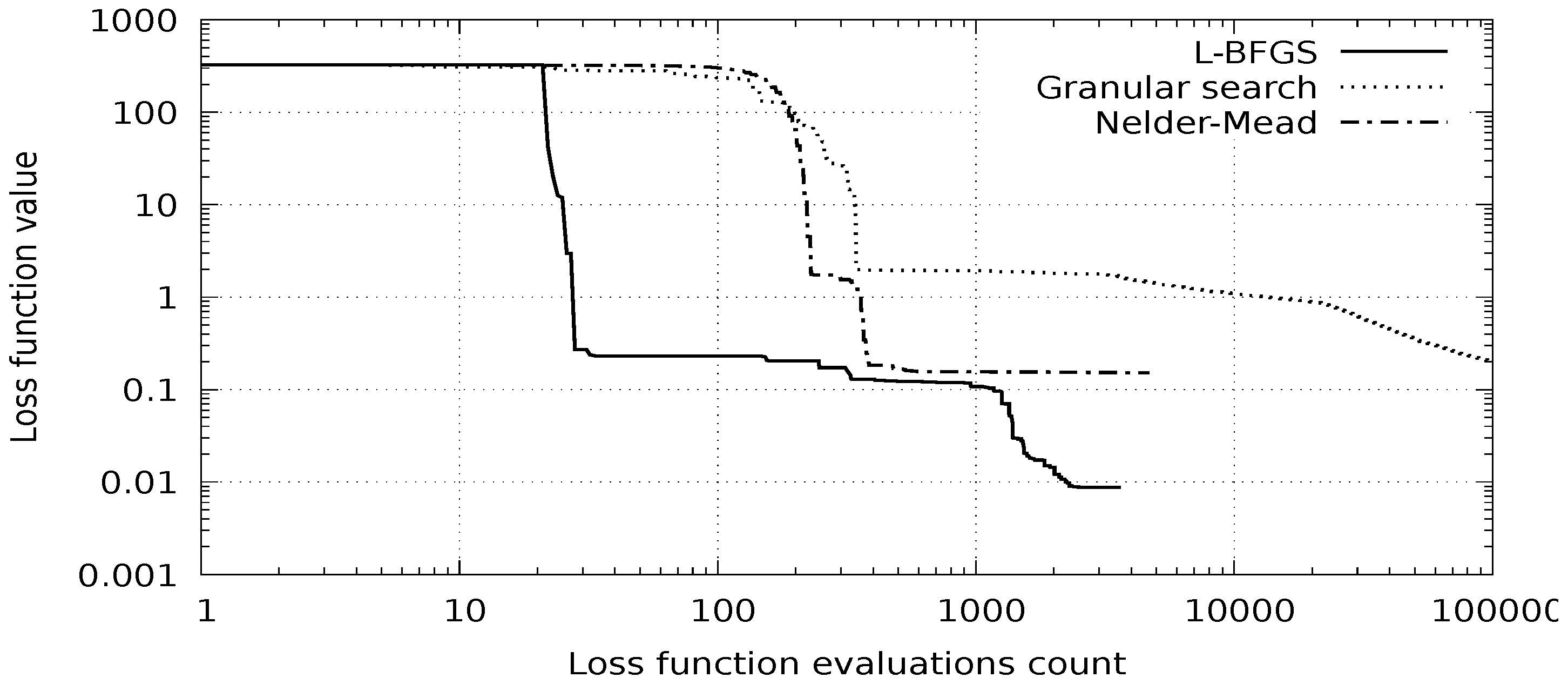
In
Figure 2, we compare the discussed method with two other methods: the Nelder–Mead method and the granular search method [
29]. Convergence of the three methods starting from the same point is presented. It can be seen that the discussed method converges much faster and is less prone to long explorations of local minima.
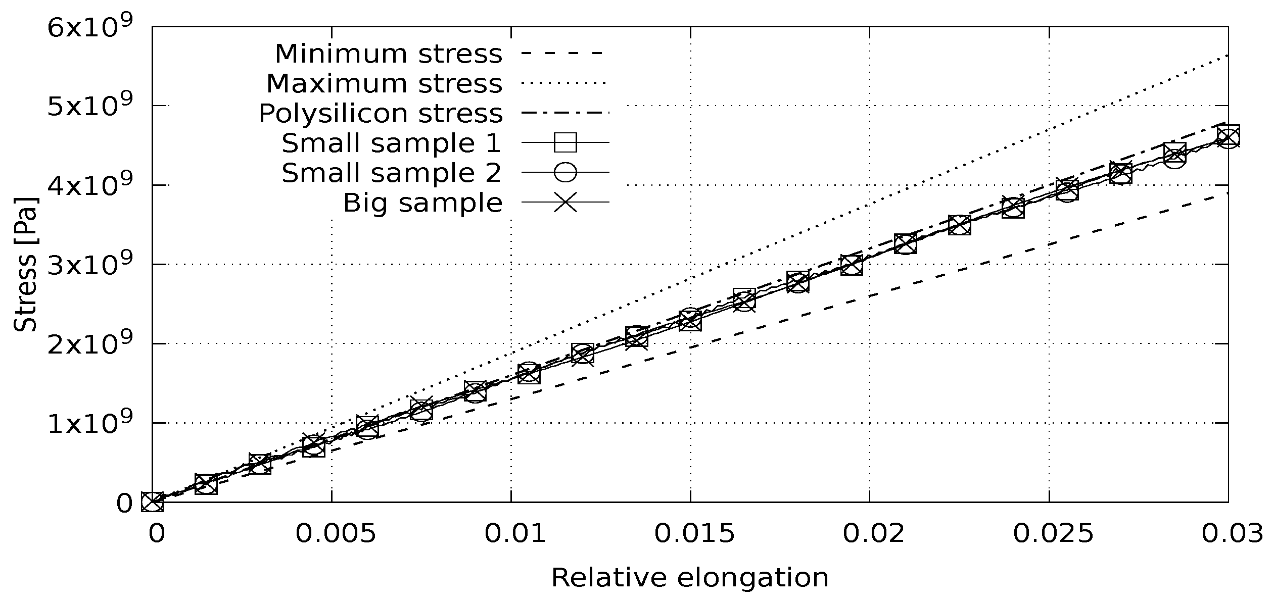
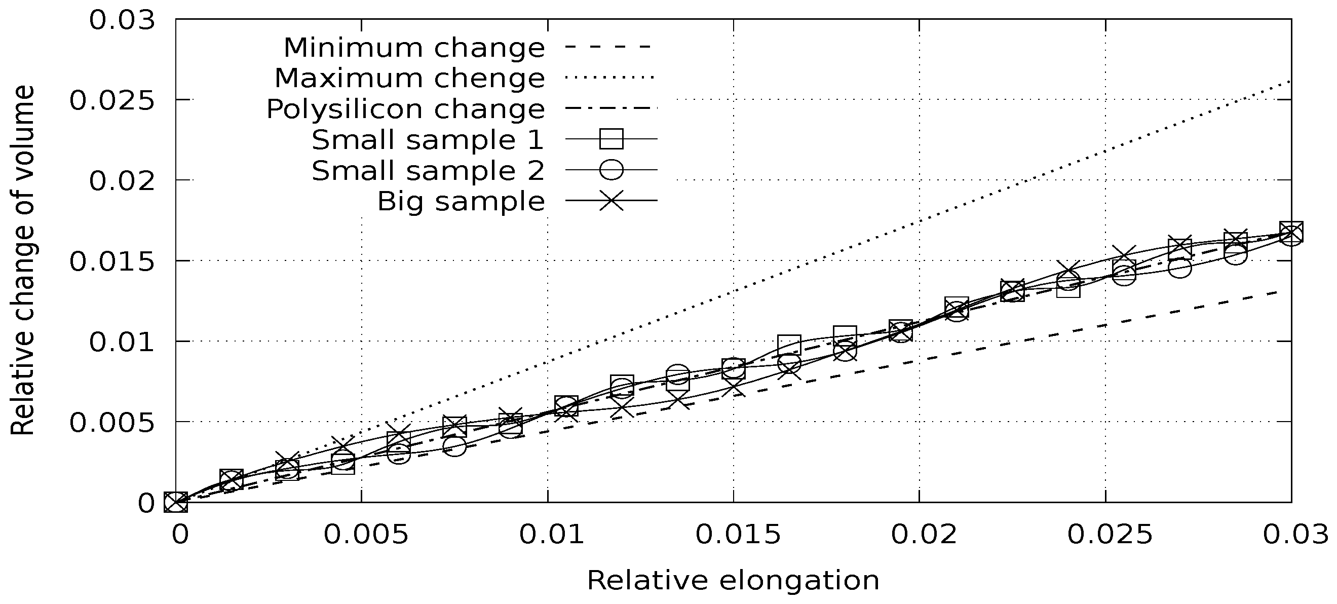
Having interatomic potential parameters, we can continue with discrete element modeling. The first group of computational experiments is focused on modeling the stress–strain state of materials. We solve the following problem: a polycrystalline silicon sample is periodically continued in one direction and stretched in that direction with a constant speed. We use a quasistatic approach; a few steps are carried out with the sample deformation, and then a few steps are performed to stabilize the sample. Three experiments were conducted with varying physical sizes and element sizes. In the first two experiments, the object was composed of 384 elements; in the third experiment, the object was composed of 3072 elements. Each element contained 64 atoms. The linear size of the object was doubled in each experiment. Base lattice orientations are independently randomized in each experiment. The stress-deformation and volume-deformation dependences were obtained, which allow for calculating Young’s modulus and Poisson’s ratio. The reference values of Young’s modulus for silicon are: crystal, 130 ÷ 188 GPa; polycrystal, 160 GPa. Poisson’s ratio values for silicon are: crystal, 0.064 ÷ 0.28; polycrystal, 0.22 [
30].
The experimental results show a good correspondence of the calculated stress and volume change with linear estimation from Young’s modulus (
Figure 3) and Poisson’s ratio (
Figure 4) that does not depend on the object size or the number of elements.
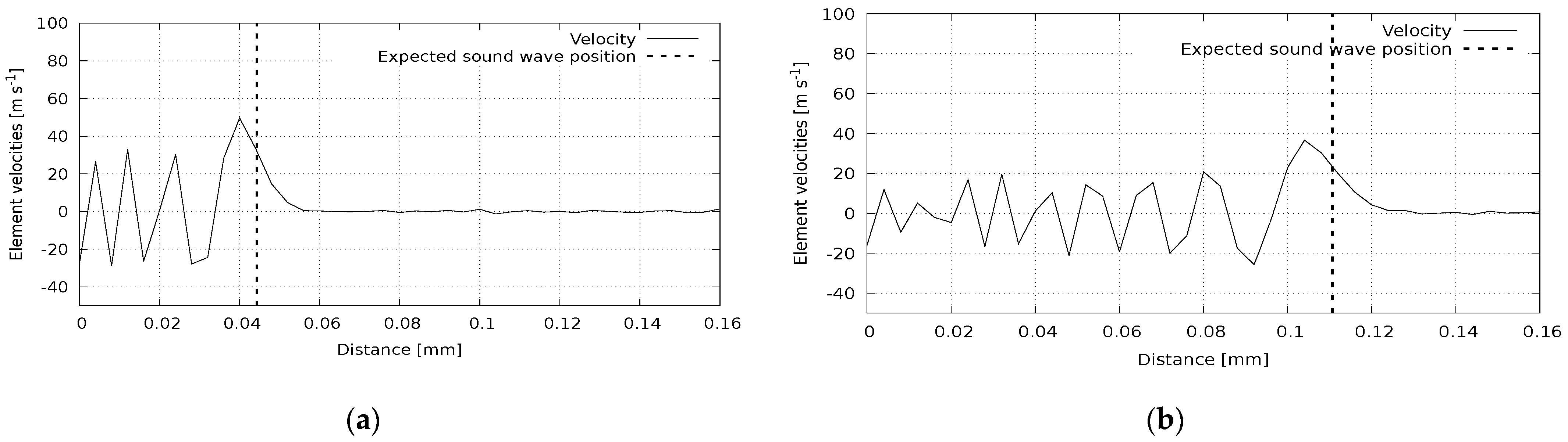
In the second group of computational experiments, we simulate the dynamic processes in materials. The number of discrete elements in all experiments was 3840, with an atomic sample size of 64 atoms. In the first experiment, the pressure wave propagation was calculated in a polycrystalline silicon plate under the action of impulse normal to the plate surface. The results at two moments are presented in
Figure 5. The reference sound speed for this case is 8850 m/s. The sound wavefront corresponding to this value is shown in the figure with a vertical line. It can be seen that the calculated wave position agrees with the reference one. A similar picture can be observed in
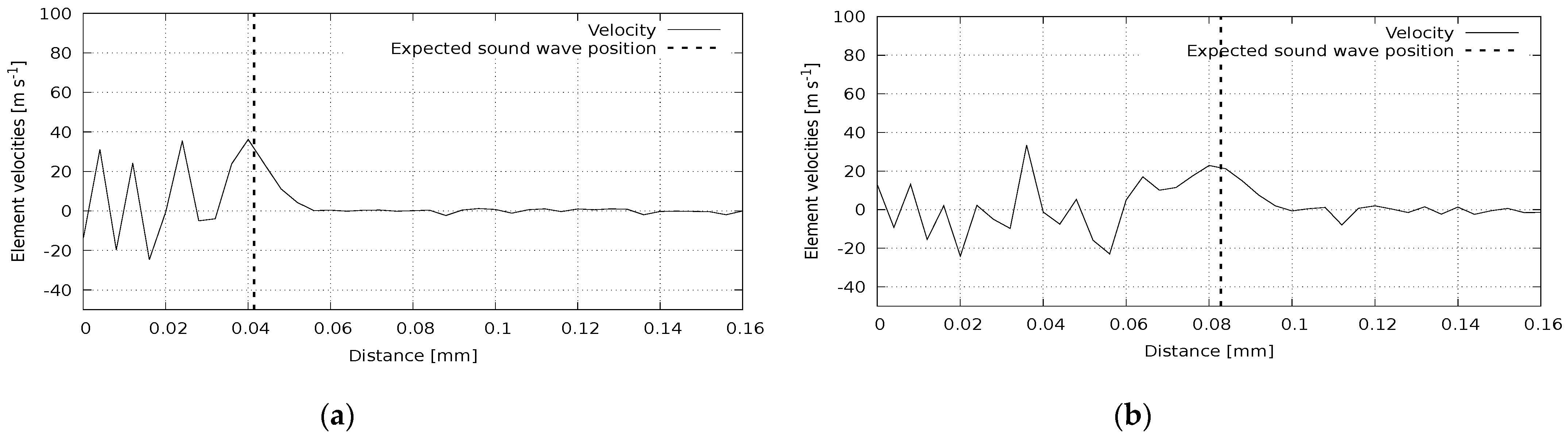
Figure 6, where we illustrate the wave propagation in a polycrystalline silicon rod affected by an instantaneous pulse in the parallel direction. The reference value here is 8290 m/s. Shear wave propagation is presented in
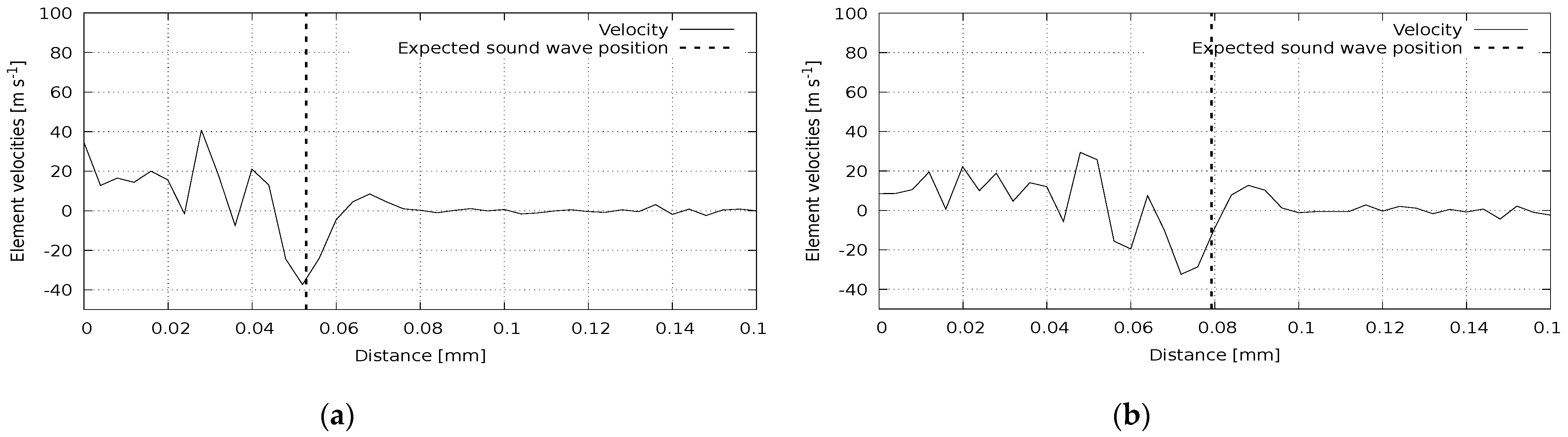
Figure 7. Here, a polycrystalline silicon rod was impacted by a perpendicular impulse. The reference value for this case is 5280 m/s. Again, we can see a good agreement of calculated and reference data.


