Primal-Dual Splitting Algorithms for Solving Structured Monotone Inclusion with Applications

Abstract

This work proposes two different primal-dual splitting algorithms for solving structured monotone inclusion containing a cocoercive operator and the parallel-sum of maximally monotone operators. In particular, the parallel-sum is symmetry. The proposed primal-dual splitting algorithms are derived from two approaches: One is the preconditioned forward–backward splitting algorithm, and the other is the forward–backward–half-forward splitting algorithm. Both algorithms have a simple calculation framework. In particular, the single-valued operators are processed via explicit steps, while the set-valued operators are computed by their resolvents. Numerical experiments on constrained image denoising problems are presented to show the performance of the proposed algorithms.

1. Introduction

In the last decade, there has been great interest in primal-dual splitting algorithms for solving structured monotone inclusion. The reason is that many convex minimization problems arising in image processing, statistical learning, and economic management can be modelled by such monotone inclusion problems. Based on the perspective of operator splitting algorithms, these primal-dual splitting algorithms can be roughly divided into four categories: (i) Forward–backward splitting type [1,2,3,4]; (ii) Douglas-Rachford splitting type [5,6,7]; (iii) Forward–backward–forward splitting type [8,9,10,11,12]; and (iv) Projective splitting type [13,14,15,16,17]. In 2014, Becker and Combettes [11] first studied the following structured monotone inclusion problem:

Problem 1.

Let $\mathcal{H}$ be a real Hilbert space, $z\in \mathcal{H}$, and $m>0$ be an integer. Let $A:\mathcal{H}\to 2^{\mathcal{H}}$ be maximally monotone and $C:\mathcal{H}\to \mathcal{H}$ be monotone and L-Lipschitzian continuous, for some $L>0$. For every integer $i=1,\dots ,m$, let ${\mathcal{X}}_i$ and ${\mathcal{G}}_i$ be real Hilbert spaces, let $B_i:{\mathcal{X}}_i\to 2^{{\mathcal{X}}_i}$ and $D_i:{\mathcal{Y}}_i\to 2^{{\mathcal{Y}}_i}$ be maximally monotone operators, and let $K_i:\mathcal{H}\to {\mathcal{X}}_i$ and $M_i:\mathcal{H}\to {\mathcal{Y}}_i$ be nonzero linear bounded operators. The problem is to solve the primal inclusion

$$find\hspace{1em}x\in \mathcal{H}such\hspace{1em}that\hspace{1em}z\in Ax+\sum _{i=1}^m\left(\left(K_i^{*}\circ B_i\circ K_i\right)\square \left(M_i^{*}\circ D_i\circ M_i\right)\right)x+Cx,$$

(1)

together with its dual inclusion  

$$find\left\{\begin{array}{c}{p}_i\in {\mathcal{X}}_i,i=1,\dots ,m,\hfill \\ q_i\in {\mathcal{Y}}_i,i=1,\dots ,m,\hfill \\ y_i\in \mathcal{H},i=1,\dots ,m,\hfill \end{array}\right.such\hspace{1em}that\exists x\in \mathcal{H}:\left\{\begin{array}{c}z-\sum _{i=1}^m{L}_i^{*}{K}_i^{*}{p}_i\in Ax+Cx,\hfill \\ K_{i}x-K_i{y}_i\in B_i^{-1}{p}_i,i=1,\dots ,m,\hfill \\ M_i{y}_i\in D_i^{-1}{q}_i,i=1,\dots ,m,\hfill \\ K_i^{*}{p}_i=M_i^{*}{q}_i,i=1,\dots ,m.\hfill \end{array}\right.$$

(2)

Based on the method of [10], they proposed a primal-dual splitting algorithm to solve (1) and (2). Moreover, they applied the algorithm to solve an image restoration model with infimal convolution terms mixing first- and second-order total variation, which was initially studied in [18] and further explored in [19]. The advantage of this model is that it can reduce the staircase effects caused by the first-order total variation. Furthermore, Boţ and Hendrich [4] studied a more general monotone inclusion problem as follows.

Problem 2.

Let $\mathcal{H}$ be a real Hilbert space, $z\in \mathcal{H}$, and $m>0$ be an integer. Let $A:\mathcal{H}\to 2^{\mathcal{H}}$ be maximally monotone and $C:\mathcal{H}\to \mathcal{H}$ be ${\mu }^{-1}$-cocoercive operator, for some $\mu >0$. For every $i=1,\dots ,m$, let ${\mathcal{G}}_i,{\mathcal{X}}_i,{\mathcal{Y}}_i$ be real Hilbert spaces, let $r_i\in {\mathcal{G}}_i$, let $B_i:{\mathcal{X}}_i\to 2^{{\mathcal{X}}_i}$ and $D_i:{\mathcal{Y}}_i\to 2^{{\mathcal{Y}}_i}$ be maximally monotone operators, and let $L_i:\mathcal{H}\to {\mathcal{G}}_i,K_i:{\mathcal{G}}_i\to {\mathcal{X}}_i$ and $M_i:{\mathcal{G}}_i\to {\mathcal{Y}}_i$ be nonzero bounded linear operators. The problem is to solve the primal inclusion

$$find x\in \mathcal{H}\mathit{such} \mathit{that} z\in Ax+\sum _{i=1}^m{L}_i^{*}\left(\left(K_i^{*}\circ B_i\circ K_i\right)\square \left(M_i^{*}\circ D_i\circ M_i\right)\right)(L_{i}x-r_i)+Cx,$$

(3)

together with its dual inclusion

$$find\left\{\begin{array}{c}{p}_i\in {\mathcal{X}}_i,i=1,\dots ,m,\hfill \\ q_i\in {\mathcal{Y}}_i,i=1,\dots ,m,\hfill \\ y_i\in {\mathcal{G}}_i,i=1,\dots ,m,\hfill \end{array}\right.such\hspace{1em}that\exists x\in \mathcal{H}:\left\{\begin{array}{c}z-\sum _{i=1}^m{L}_i^{*}{K}_i^{*}{p}_i\in Ax+Cx,\hfill \\ K_i\left(L_{i}x-y_i-r_i\right)\in B_i^{-1}{p}_i,i=1,\dots ,m,\hfill \\ M_i{y}_i\in D_i^{-1}{q}_i,i=1,\dots ,m,\hfill \\ K_i^{*}{p}_i=M_i^{*}{q}_i,i=1,\dots ,m.\hfill \end{array}\right.$$

(4)

It is easy to see that Problem 1 could be viewed as a special case of Problem 2 by letting $L_i=I$ and $r_i=0$, for any $i=1,\cdots ,m$. They proposed two different primal-dual algorithms for solving the primal-dual pair of monotone inclusions (3) and (4). The first algorithm is a forward–backward splitting type, which is defined as follows. Let $x_0\in \mathcal{H}$, and for any $i=1,\dots ,m$, $p_{i,0}\in {\mathcal{X}}_i$, $q_{i,0}\in {\mathcal{Y}}_i$ and $z_{i,0},y_{i,0},v_{i,0}\in {\mathcal{G}}_i$, and set

$$(\forall n\ge 0)⌊\begin{array}{cc}\hfill & {\tilde{x}}_n=J_{\tau A}(x_n-\tau (C{x}_n+\sum _{i=1}^m{L}_i^{*}{v}_{i,n}-z))\hfill \\ \hfill & \mathrm{for}i=1,\dots ,m\hfill \\ \hfill & ⌊\begin{array}{cc}\hfill & {\tilde{p}}_{i,n}=J_{{\theta }_{1,i}{B}_i^{-1}}\left(p_{i,n}+{\theta }_{1,i}{K}_i{z}_{i,n}\right)\hfill \\ \hfill & {\tilde{q}}_{i,n}=J_{{\theta }_{2,i}{D}_i^{-1}}\left(q_{i,n}+{\theta }_{2,i}{M}_i{y}_{i,n}\right)\hfill \\ \hfill & u_{1,i,n}=z_{i,n}+{\gamma }_{1,i}\left(K_i^{*}\left(p_{i,n}-2{\tilde{p}}_{i,n}\right)+v_{i,n}+{\sigma }_i\left(L_i\left(2{\tilde{x}}_n-x_n\right)-r_i\right)\right)\hfill \\ \hfill & u_{2,i,n}=y_{i,n}+{\gamma }_{2,i}\left(M_i^{*}\left(q_{i,n}-2{\tilde{q}}_{i,n}\right)+v_{i,n}+{\sigma }_i\left(L_i\left(2{\tilde{x}}_n-x_n\right)-r_i\right)\right)\hfill \\ \hfill & {\tilde{z}}_{i,n}=\frac{1+{\sigma }_i{\gamma }_{2,i}}{1+{\sigma }_i\left({\gamma }_{1,i}+{\gamma }_{2,i}\right)}(u_{1,i,n}-\frac{{\sigma }_i{\gamma }_{1,i}}{1+{\sigma }_i{\gamma }_{2,i}}{u}_{2,i,n})\hfill \\ \hfill & {\tilde{y}}_{i,n}=\frac{1}{1+{\sigma }_i{\gamma }_{2,i}}\left(u_{2,i,n}-{\sigma }_i{\gamma }_{2,i}{\tilde{z}}_{i,n}\right)\hfill \\ \hfill & {\tilde{v}}_{i,n}=v_{i,n}+{\sigma }_i\left(L_i\left(2{\tilde{x}}_n-x_n\right)-r_i-{\tilde{z}}_{i,n}-{\tilde{y}}_{i,n}\right)\hfill \end{array}\hfill \\ \hfill & x_{n+1}=x_n+{\lambda }_n\left({\tilde{x}}_n-x_n\right)\hfill \\ \hfill & \mathrm{for} i=1,\dots ,m\hfill \\ \hfill & ⌊\begin{array}{cc}\hfill & p_{i,n+1}=p_{i,n}+{\lambda }_n\left({\tilde{p}}_{i,n}-p_{i,n}\right)\hfill \\ \hfill & q_{i,n+1}=q_{i,n}+{\lambda }_n\left({\tilde{q}}_{i,n}-q_{i,n}\right)\hfill \\ \hfill & z_{i,n+1}=z_{i,n}+{\lambda }_n\left({\tilde{z}}_{i,n}-z_{i,n}\right)\hfill \\ \hfill & y_{i,n+1}=y_{i,n}+{\lambda }_n\left({\tilde{y}}_{i,n}-y_{i,n}\right)\hfill \\ \hfill & v_{i,n+1}=v_{i,n}+{\lambda }_n\left({\tilde{v}}_{i,n}-v_{i,n}\right),\hfill \end{array}\hfill \end{array}$$

(5)

where for any $i=1,\dots ,m$, $\tau ,{\theta }_{1,i},{\theta }_{2,i},{\gamma }_{1,i},{\gamma }_{2,i}$ and ${\sigma }_i$ are strictly positive real numbers such that

$$2{\mu }^{-1}(1-\overline{\alpha })\underset{i=1,\dots ,m}{min}\left\{\frac{1}{\tau },\frac{1}{{\theta }_{1,i}},\frac{1}{{\theta }_{2,i}},\frac{1}{{\gamma }_{1,i}},\frac{1}{{\gamma }_{2,i}},\frac{1}{{\sigma }_i}\right\}>1$$

(6)

for

$$\overline{\alpha }=max\left\{\sqrt{\tau \sum _{i=1}^m{\sigma }_i{∥L_i∥}^2},\underset{j=1,\dots ,m}{max}\left\{\sqrt{{\theta }_{1,j}{\gamma }_{1,j}{∥K_j∥}^2},\sqrt{{\theta }_{2,j}{\gamma }_{2,j}{∥M_j∥}^2}\right\}\right\}.$$

(7)

In addition, $\left\{{\lambda }_n\right\}\subseteq [\epsilon ,1]$, where $\epsilon \in (0,1)$. The second algorithm is a forward–backward–forward splitting type. Let $x_0\in \mathcal{H}$, and for any $i=1,\dots ,m$, let $p_{i,0}\in {\mathcal{X}}_i,q_{i,0}\in {\mathcal{Y}}_i$, $z_{i,0},y_{i,0},v_{i,0}\in {\mathcal{G}}_i$, and set  

$$(\forall n\ge 0)⌊\begin{array}{cc}\hfill & {\tilde{x}}_n=J_{{\gamma }_{n}A}(x_n-{\gamma }_n(C{x}_n+\sum _{i=1}^m{L}_i^{*}{v}_{i,n}-z))\hfill \\ \hfill & \mathrm{for} i=1,\dots ,m\hfill \\ \hfill & ⌊\begin{array}{cc}\hfill & {\tilde{p}}_{i,n}=J_{{\gamma }_n{B}_i^{-1}}\left(p_{i,n}+{\gamma }_n{K}_i{z}_{i,n}\right)\hfill \\ \hfill & {\tilde{q}}_{i,n}=J_{{\gamma }_n{D}_i^{-1}}\left(q_{i,n}+{\gamma }_n{M}_i{y}_{i,n}\right)\hfill \\ \hfill & u_{1,i,n}=z_{i,n}-{\gamma }_n\left(K_i^{*}{p}_{i,n}-v_{i,n}-{\gamma }_n\left(L_i{x}_n-r_i\right)\right)\hfill \\ \hfill & u_{2,i,n}=y_{i,n}-{\gamma }_n\left(M_i^{*}{q}_{i,n}-v_{i,n}-{\gamma }_n\left(L_i{x}_n-r_i\right)\right)\hfill \\ \hfill & {\tilde{z}}_{i,n}=\frac{1+{\gamma }_n^2}{1+2{\gamma }_n^2}(u_{1,i,n}-\frac{{\gamma }_n^2}{1+{\gamma }_n^2}{u}_{2,i,n})\hfill \\ \hfill & {\tilde{y}}_{i,n}=\frac{1}{1+{\gamma }_n^2}\left(u_{2,i,n}-{\gamma }_n^2{\tilde{z}}_{i,n}\right)\hfill \\ \hfill & {\tilde{v}}_{i,n}=v_{i,n}+{\gamma }_n\left(L_i{x}_n-r_i-{\tilde{z}}_{i,n}-{\tilde{y}}_{i,n}\right)\hfill \end{array}\hfill \\ \hfill & x_{n+1}={\tilde{x}}_n+{\gamma }_n(C{x}_n-C{\tilde{x}}_n+\sum _{i=1}^m{L}_i^{*}\left(v_{i,n}-{\tilde{v}}_{i,n}\right))\hfill \\ \hfill & \mathrm{for} i=1,\dots ,m\hfill \\ \hfill & ⌊\begin{array}{cc}\hfill & p_{i,n+1}={\tilde{p}}_{i,n}-{\gamma }_n\left(K_i\left(z_{i,n}-{\tilde{z}}_{i,n}\right)\right)\hfill \\ \hfill & q_{i,n+1}={\tilde{q}}_{i,n}-{\gamma }_n\left(M_i\left(y_{i,n}-{\tilde{y}}_{i,n}\right)\right)\hfill \\ \hfill & z_{i,n+1}={\tilde{z}}_{i,n}+{\gamma }_n\left(K_i^{*}\left(p_{i,n}-{\tilde{p}}_{i,n}\right)\right)\hfill \\ \hfill & y_{i,n+1}={\tilde{y}}_{i,n}+{\gamma }_n\left(M_i^{*}\left(q_{i,n}-{\tilde{q}}_{i,n}\right)\right)\hfill \\ \hfill & v_{i,n+1}={\tilde{v}}_{i,n}-{\gamma }_n\left(L_i\left(x_n-{\tilde{x}}_n\right)\right),\hfill \end{array}\hfill \end{array}$$

(8)

where $\left\{{\gamma }_n\right\}\subseteq \left[\epsilon ,\frac{1-\epsilon }{\beta }\right]$ with $\epsilon \in \left(0,\frac{1}{\beta +1}\right)$ and

$$\beta =\mu +\sqrt{max\left\{\sum _{i=1}^m{∥L_i∥}^2,{max}_{j=1,\dots ,m}\left\{{∥K_j∥}^2,{∥M_j∥}^2\right\}\right\}}.$$

(9)

The first algorithm (5) could be viewed as a preconditioned forward–backward splitting algorithm [20]. While the second algorithm (8) is an instance of the forward-backward-forward splitting algorithm proposed by Tseng [21]. We can see that the operators $B_i^{-1}$ and $D_i^{-1}$ are symmetry in both of algorithms. We call the first algorithm (5) the FB_BH algorithm and the second algorithm, the FBF_BH algorithm.

In this paper, we continue studying primal-dual splitting algorithms for solving the structured monotone inclusion (3) and (4). First, we establish a new convergence theorem for the primal-dual forward–backward splitting type algorithm (5). We relax the limitation of the iteration parameters as well as expand the selection range of the relaxation parameter. Since the primal-dual forward–backward–forward splitting type algorithm (8) does not make full use of the cocoercive operator, we introduce a new primal-dual splitting algorithm for solving (3) and (4), which is based on the forward–backward–half-forward splitting algorithm [22]. This new algorithm is not only less computationally expensive than the original algorithm but also provides a larger range of parameter selection. To show the advantages of the proposed algorithms, we apply them to solve image denoising problems.

This paper is organized as follows. In Section 2, we recall some preliminary results in monotone operator theory. In Section 3, we present the main results. We study the convergence of two primal-dual splitting algorithms for solving (3) and (4). Furthermore, we employ the obtained algorithms to solve convex minimization problems. In Section 4, we perform numerical experiments on image denoising problems. Finally, we present conclusions.

2. Preliminaries

Throughout this paper, $\mathcal{H}$ is a real Hilbert space, which is equipped with inner product $\langle ·,·\rangle$ and associated norm $\parallel ·\parallel =\sqrt{\langle ·,·\rangle }$. Let $2^{\mathcal{H}}$ be the power set of $\mathcal{H}$. Let $L:\mathcal{H}\to \mathcal{G}$ be a linear bounded operator, where $\mathcal{G}$ is another real Hilbert space, the operator $L^{*}:\mathcal{G}\to \mathcal{H}$ is said to be its adjoint if $\langle Lx,y\rangle =〈x,L^{*}y〉$ holds for all $x\in \mathcal{H}$ and all $y\in \mathcal{G}$. Most of the definitions are taken from [23].

Let $A:\mathcal{H}\to 2^{\mathcal{H}}$ be a set-valued operator. Let zer $A=\{x\in \mathcal{H}:0\in Ax\}$ be the set of its zeros, ran $A=\{u\in \mathcal{H}:$$\exists x\in \mathcal{H},u\in Ax\}$ its range, and gra $A=\left\{\right(x,u)\in \mathcal{H}\times \mathcal{H}:u\in Ax\}$ its graph. The inverse of A is defined by $A^{-1}:\mathcal{H}\to 2^{\mathcal{H}},u\mapsto \{x\in \mathcal{H}:u\in Ax\}$.

Definition 1.

Let $A:\mathcal{H}\to 2^{\mathcal{H}}$ be a set-valued operator. A is said to be monotone, if $\langle x-y,u-v\rangle \ge 0,\forall (x,u),(y,v)\in graA.$ Furthermore, A is said to be maximally monotone if it is monotone, and there exists no monotone operator $B:\mathcal{H}\to 2^{\mathcal{H}}$ such that gra B properly contains gra A.

Definition 2.

Let $T:\mathcal{H}\to \mathcal{H}$ be a single-valued operator.

(i) T is said to be L-Lipschitzian, for some $L>0$, if $\parallel Tx-Ty\parallel \le L\parallel x-y\parallel ,\forall x,y\in \mathcal{H}.$

(ii) T is said to be μ-cocoercive, for some $\mu >0$, if $\langle x-y,Tx-Ty\rangle \ge {\mu \parallel Tx-Ty\parallel }^2,$$\forall x,y\in \mathcal{H}.$

Definition 3.

Let $A:\mathcal{H}\to 2^{\mathcal{H}}$, the resolvent of A with index $\lambda >0$ is defined by

$$J_{\lambda A}={(Id+\lambda A)}^{-1},$$

(10)

where $Id$ denotes the identity operator on $\mathcal{H}$.

Definition 4.

Let $A_1,A_2:\mathcal{H}\to 2^{\mathcal{H}}$ be two set-valued operators. The sum and the parallel sum of $A_1$ and $A_2$ are defined as follows:

$$\begin{array}{cc}\hfill & A_1+A_2:\mathcal{H}\to 2^{\mathcal{H}},\left(A_1+A_2\right)\left(x\right)=A_1\left(x\right)+A_2\left(x\right)\hfill \\ \hfill & A_1\square A_2:\mathcal{H}\to 2^{\mathcal{H}},A_1\square A_2={\left(A_1^{-1}+A_2^{-1}\right)}^{-1}.\hfill \end{array}$$

(11)

Let $f:\mathcal{H}\to \overline{\mathbb{R}}:=\mathbb{R}\cup \{\pm \infty \}$. We denote its effective domain as dom $f:=\{x\in \mathcal{H}:f(x)<+\infty \}$, f is said to be proper if $domf\ne ⌀$ and $f\left(x\right)>-\infty$ for all $x\in \mathcal{H}$. Furthermore, we define ${\mathsf{\Gamma }}_0\left(\mathcal{H}\right):=\{f:\mathcal{H}\to \overline{\mathbb{R}}\mid f$ is proper, convex, and lower semicontinuous (lsc)}.

The conjugate function of f is defined by $f^{*}:\mathcal{H}\to \overline{\mathbb{R}},f^{*}\left(p\right)=sup\{\langle p,x\rangle -f\left(x\right):x\in \mathcal{H}\}$ for all $p\in \mathcal{H}$. If $f\in {\mathsf{\Gamma }}_0\left(\mathcal{H}\right)$, then $f^{**}=f$.

Let $f\in {\mathsf{\Gamma }}_0\left(\mathcal{H}\right)$, the subdifferential of f is defined by $\partial f:\mathcal{H}\to 2^{\mathcal{H}}:x\mapsto \{u\in \mathcal{H}\mid (\forall y\in \mathcal{H})f\left(y\right)\ge f\left(x\right)+\langle u\mid y-x\rangle \}$. If $f\in {\mathsf{\Gamma }}_0\left(\mathcal{H}\right)$, then $\partial f$ is maximally monotone.

Let two proper functions $f,h:\mathcal{H}\to \overline{\mathbb{R}}$,

$$f\square h:\mathcal{H}\to \overline{\mathbb{R}},(f\square h)\left(x\right)=\underset{y\in \mathcal{H}}{inf}\{f\left(y\right)+h(x-y)\},$$

(12)

denotes their infimal convolution.

Let $f\in {\mathsf{\Gamma }}_0\left(\mathcal{H}\right)$ and $\gamma >0$, the proximity operator of f is defined by

$${prox}_{\gamma f}:\mathcal{H}\to \mathcal{H}:x\mapsto \underset{y\in \mathcal{H}}{argmin}\left\{f\left(y\right)+\frac{1}{2\gamma }{\parallel x-y\parallel }^2\right\}.$$

(13)

It follows from $f\in {\mathsf{\Gamma }}_0\left(\mathcal{H}\right)$ that ${prox}_{\gamma f}\left(x\right)=J_{\gamma \partial f}\left(x\right)$.

The following lemma shows the relationship between the proximity operator of f and its convex conjugate $f^{*}$.

Lemma 1. 

(Moreau’s decomposition) Let $\gamma >0$ and $f\in {\mathsf{\Gamma }}_0\left(\mathcal{H}\right)$, then

$${prox}_{\gamma f}\left(x\right)+\gamma {prox}_{\frac{1}{\gamma }{f}^{*}}\left(\frac{1}{\gamma }x\right)=x,\forall x\in \mathcal{H}.$$

Let $C\subseteq \mathcal{H}$ be a nonempty closed convex set, the indicator function of C is denoted by

$${\delta }_C:x\mapsto \left\{\begin{array}{c}0,\mathrm{if}x\in C\hfill \\ +\infty ,\mathrm{otherwise}.\hfill \end{array}\right.$$

(14)

The orthogonal projection onto C is defined by $P_C$, which is $P_C\left(x\right)=\underset{y\in C}{argmin}\parallel x-y\parallel$. Let $\gamma >0$, ${prox}_{\gamma {\delta }_C}\left(x\right)=P_C\left(x\right)$.

3. Main Results

In this section, we study primal-dual splitting algorithms for solving (3) and (4) and discuss their asymptotic convergence. First, we provide a technique lemma, which shows that the primal-dual monotone inclusions (3) and (4) are equivalent to the sum of three maximally monotone operators. In the following, let $\mathcal{H}={\mathcal{H}}_1\oplus \cdots {\mathcal{H}}_m$ be the direct sum of real Hilbert spaces ${\left\{{\mathcal{H}}_i\right\}}_{i=1}^m$. Let $\mathit{v}=(v_1,\cdots ,v_m)\in \mathcal{H}$ and $\mathit{q}=(q_1,\cdots ,q_m)\in \mathcal{H}$, the inner product and associated norm on $\mathcal{H}$ are defined as

$${\langle \mathit{v},\mathit{q}\rangle }_{\mathcal{H}}=\sum _{i=1}^m\langle v_i,q_i\rangle ,{\parallel \mathit{v}\parallel }_{\mathcal{H}}=\sqrt{\sum _{i=1}^m{\parallel v_i\parallel }^2}.$$

Lemma 2.

Let $\mathcal{H}$, A, C, ${\mathcal{X}}_i$, ${\mathcal{Y}}_i$, ${\mathcal{G}}_i$, $B_i$, $D_i$, $L_i$, $K_i$, $M_i$, $i=1,\cdots ,m$ be defined as in Problem 2, and let

$$\begin{array}{cc}\hfill & \mathit{X}:={\mathcal{X}}_1\oplus \cdots \oplus {\mathcal{X}}_m,\mathcal{Y}:={\mathcal{Y}}_1\oplus \cdots \oplus {\mathcal{Y}}_m,\mathcal{G}:={\mathcal{G}}_1\oplus \cdots \oplus {\mathcal{G}}_m,\mathcal{K}:=\mathcal{H}\oplus \mathcal{X}\oplus \mathcal{Y}\oplus \mathcal{G}\oplus \mathcal{G}\oplus \mathcal{G},\hfill \\ \hfill & \mathit{p}=\left(p_1,\dots ,p_m\right)\in \mathcal{X},\mathit{q}=\left(q_1,\dots ,q_m\right)\in \mathcal{Y},\mathit{z}=\left(z_1,\dots ,z_m\right)\in \mathcal{G},\hfill \\ \hfill & \mathit{y}=\left(y_1,\dots ,y_m\right)\in \mathcal{G},\mathit{v}=\left(v_1,\dots ,v_m\right)\in \mathcal{G},\mathit{r}=\left(r_1,\dots ,r_m\right)\in \mathcal{G},\hfill \\ \hfill & \mathit{B}:\mathcal{X}\to 2^{\mathcal{X}}:\mathit{p}\mapsto \left(B_1{p}_1,\cdots ,B_m{p}_m\right),\mathit{D}:\mathcal{Y}\to 2^{\mathcal{Y}},\mathit{q}\mapsto \left(D_1{q}_1,\cdots ,D_m{q}_m\right),\hfill \\ \hfill & \tilde{M}:\mathcal{G}\to \mathcal{Y},\mathit{y}\mapsto \left(M_1{y}_1,\cdots ,M_m{y}_m\right),\tilde{K}:\mathcal{G}\to \mathcal{X},\mathit{y}\mapsto \left(K_1{y}_1,\cdots ,K_m{y}_m\right),\hfill \\ \hfill & \mathit{M}:\mathcal{K}\to 2^{\mathcal{K}},(x,\mathit{p},\mathit{q},\mathit{z},\mathit{y},\mathit{v})\mapsto (-z+Ax)\times {\mathit{B}}^{-1}\mathit{p}\times {\mathit{D}}^{-1}\mathit{q}\times (-\mathit{v},-\mathit{v},\mathit{r}+\mathit{z}+\mathit{y})\hfill \\ \hfill & \mathit{S}:\mathcal{K}\to \mathcal{K},(x,\mathit{p},\mathit{q},\mathit{z},\mathit{y},\mathit{v})\mapsto \left(\sum _{i=1}^m{L}_i^{*}{v}_i,-\tilde{K}\mathit{z},-\tilde{M}\mathit{y},{\tilde{K}}^{*}\mathit{p},{\tilde{M}}^{*}\mathit{q},-L_{1}x,\dots ,-L_{m}x\right)\hfill \\ \hfill & \mathit{Q}:\mathcal{K}\to \mathcal{K},(x,\mathit{p},\mathit{q},\mathit{z},\mathit{y},\mathit{v})\mapsto (Cx,\mathbf{0},\mathbf{0},\mathbf{0},\mathbf{0},\mathbf{0})\hfill \end{array}$$

(15)

Then the following conclusions hold:

(i)

$\mathit{M}$ is maximally monotone.

(ii)

$\mathit{S}$ is monotone and l-Lipschitzian, where

$$l=(max\{\underset{i=1,\cdots ,m}{max}\parallel K_i{\parallel }^2,\underset{i=1,\cdots ,m}{max}\parallel M_i{\parallel }^2,\sum _{i=1}^m\parallel L_i{\parallel }^2{\left\}\right)}^{\frac{1}{2}}.$$

(16)

(iii)

$\mathit{Q}$ is ${\mu }^{-1}$-cocoercive.

(iv)

For any $\overline{x}\in \mathcal{H}$, $\overline{x}$ is a solution to Problem 2, if and only if $\overline{x}\in zer(\mathit{M}+\mathit{S}+\mathit{Q})$.

Proof. 

(i) Since $\mathit{A},\mathit{B}$, and $\mathit{D}$ are maximally monotone, it follows from [23] Proposition $20.22$ and Proposition $20.23$ that the set-valued operator $\mathit{M}$ is maximally monotone.

(ii) By taking two arbitrary elements $\mathit{x}=(x,\mathit{p},\mathit{q},\mathit{z},\mathit{y},\mathit{v})$ and $\widehat{\mathit{x}}=(\widehat{x},\widehat{\mathit{p}},\widehat{\mathit{q}},\widehat{\mathit{z}},\widehat{\mathit{y}},\widehat{\mathit{v}})$ in $\mathcal{K}$, we obtain

$$\begin{array}{cc}\hfill & \langle \mathit{x}-\widehat{\mathit{x}},\mathit{S}\mathit{x}-\mathit{S}\widehat{\mathit{x}}\rangle \hfill \\ \hfill =& \langle (x-\widehat{x},p_1-{\widehat{p}}_1,\cdots ,p_m-{\widehat{p}}_m,q_1-{\widehat{q}}_1,\cdots ,q_m-{\widehat{q}}_m,z_1-{\widehat{z}}_1,\cdots ,z_m-{\widehat{z}}_m,y_1-{\widehat{y}}_1,\cdots ,y_m-{\widehat{y}}_m,\hfill \\ \hfill & v_1-{\widehat{v}}_1,\cdots ,v_m-{\widehat{v}}_m),(\sum _{i=1}^m{L}_i^{*}(v_i-{\widehat{v}}_i),-K_1(z_1-{\widehat{z}}_1),\cdots ,-K_m(z_m-{\widehat{z}}_m),-M_1(y_1-{\widehat{y}}_1),\cdots ,-M_m(y_m-{\widehat{y}}_m),\hfill \\ \hfill & K_1^{*}(p_1-{\widehat{p}}_1),\cdots ,K_m^{*}(p_m-{\widehat{p}}_m),M_1^{*}(q_1-{\widehat{q}}_1),\cdots ,M_m^{*}(q_m-{\widehat{q}}_m),-L_1(x-\widehat{x}),\cdots ,-L_m(x-\widehat{x})\rangle \hfill \\ \hfill =& \sum _{i=1}^m\langle x-\widehat{x},L_i^{*}(v_i-{\widehat{v}}_i)\rangle -\sum _{i=1}^m\langle p_i-{\widehat{p}}_i,K_i(z_i-\widehat{z_i})\rangle -\sum _{i=1}^m\langle q_i-{\widehat{q}}_i,M_i(y_i-{\widehat{y}}_i)\rangle +\sum _{i=1}^m\langle z_i-{\widehat{z}}_i,K_i^{*}(p_i-{\widehat{p}}_i)\rangle \hfill \\ \hfill & +\sum _{i=1}^m\langle y_i-{\widehat{y}}_i,M_i^{*}(q_i-\widehat{q_i})-\sum _{i=1}^m\langle v_i-{\widehat{v}}_i,L_i(x-\widehat{x})\rangle \hfill \\ \hfill =& 0,\hfill \end{array}$$

(17)

which means that $\mathit{S}$ is monotone. It follows from the Cauchy-Schwarz inequality that

$$\begin{array}{cc}\hfill & \parallel \mathit{S}\mathit{x}-\mathit{S}\widehat{\mathit{x}}\parallel \hfill \\ \hfill & =\parallel (\sum _{i=1}^m{L}_i^{*}(v_i-{\widehat{v}}_i),-K_1(z_1-{\widehat{z}}_1),\cdots ,-K_m(z_m-{\widehat{z}}_m),-M_1(y_1-{\widehat{y}}_1),\cdots ,-M_m(y_m-{\widehat{y}}_m),\hfill \\ \hfill & +K_1^{*}(p_1-{\widehat{p}}_1),\cdots ,K_m^{*}(p_m-{\widehat{p}}_m),M_1^{*}(q_1-{\widehat{q}}_1),\cdots ,M_m^{*}(q_m-{\widehat{q}}_m),-L_1(x-\widehat{x}),\cdots ,-L_m(x-\widehat{x})\parallel \hfill \\ \hfill & =(\parallel \sum _{i=1}^m{L}_i^{*}(v_i-{\widehat{v}}_i){\parallel }^2+\sum _{i=1}^m\parallel K_i(z_i-\widehat{z_i}){\parallel }^2+\sum _{i=1}^m\parallel M_i(y_i-{\widehat{y}}_i){\parallel }^2+\sum _{i=1}^m\parallel K_i^{*}(p_i-\widehat{p_i}){\parallel }^2\hfill \\ \hfill & +\sum _{i=1}^m\parallel M_i^{*}(q_i-\widehat{q_i}){\parallel }^2+\sum _{i=1}^m\parallel L_i^{*}(x-\widehat{x}){{\parallel }^2)}^{\frac{1}{2}}\hfill \\ \hfill & \le \left(\right(\sum _{i=1}^m\parallel L_i{\parallel }^2)\sum _{i=1}^m\parallel v_i-{\widehat{v}}_i{\parallel }^2+\sum _{i=1}^m\parallel K_i{\parallel }^2\parallel z_i-\widehat{z_i}{\parallel }^2+\sum _{i=1}^m\parallel M_i{\parallel }^2\parallel y_i-{\widehat{y}}_i{\parallel }^2+\sum _{i=1}^m\parallel K_i{\parallel }^2{\parallel p_i-{\widehat{p}}_i\parallel }^2\hfill \\ \hfill & +\sum _{i=1}^m\parallel M_i{\parallel }^2\parallel q_i-{\widehat{q}}_i{\parallel }^2+\sum _{i=1}^m\parallel L_i{\parallel }^2\parallel x-\widehat{x}{{\parallel }^2)}^{\frac{1}{2}}\hfill \\ \hfill & \le \left(\right(\sum _{i=1}^m\parallel L_i{\parallel }^2)\sum _{i=1}^m\parallel v_i-{\widehat{v}}_i{\parallel }^2+\underset{i=1,\cdots ,m}{max}\parallel K_i{\parallel }^2\sum _{i=1}^m\parallel z_i-{\widehat{z}}_i{\parallel }^2+\underset{i=1,\cdots ,m}{max}\parallel M_i{\parallel }^2\sum _{i=1}^m{\parallel y_i-\widehat{y_i}\parallel }^2\hfill \\ \hfill & +\underset{i=1,\cdots ,m}{max}\parallel K_i{\parallel }^2\sum _{i=1}^m\parallel p_i-{\widehat{p}}_i{\parallel }^2+\underset{i=1,\cdots ,m}{max}\parallel M_i{\parallel }^2\sum _{i=1}^m\parallel q_i-{\widehat{q}}_i{\parallel }^2+\sum _{i=1}^m\parallel L_i{\parallel }^2\parallel x-\widehat{x}{{\parallel }^2)}^{\frac{1}{2}}\hfill \\ \hfill & \le l(\parallel x-\widehat{x}{\parallel }^2+\sum _{i=1}^m\parallel p_i-{\widehat{p}}_i{\parallel }^2+\sum _{i=1}^m\parallel q_i-{\widehat{q}}_i{\parallel }^2+\sum _{i=1}^m\parallel z_i-{\widehat{z}}_i{\parallel }^2+\sum _{i=1}^m\parallel y_i-{\widehat{y}}_i{\parallel }^2+\sum _{i=1}^m\parallel v_i-{\widehat{v}}_i{{\parallel }^2)}^{\frac{1}{2}}\hfill \\ \hfill & =l\parallel \mathit{x}-\widehat{\mathit{x}}\parallel .\hfill \end{array}$$

(18)

Hence, $\mathit{S}$ is monotone and l-Lipschitzian.

(iii) Let $\mathit{x}=(x,\mathit{p},\mathit{q},\mathit{z},\mathit{y},\mathit{v})\in \mathcal{K}$ and $\widehat{\mathit{x}}=(\widehat{x},\widehat{\mathit{p}},\widehat{\mathit{q}},\widehat{\mathit{z}},\widehat{\mathit{y}},\widehat{\mathit{v}})\in \mathcal{K}$. Since C is ${\mu }^{-1}$-cocoercive, we have

$$\begin{array}{cc}\hfill & \langle \mathit{x}-\widehat{\mathit{x}},\mathit{Q}\mathit{x}-\mathit{Q}\widehat{\mathit{x}}\rangle \ge \langle x-\widehat{x},Cx-C\widehat{x}\rangle \hfill \\ \hfill & \ge {\mu }^{-1}\parallel Cx-C\widehat{x}{\parallel }^2={\mu }^{-1}{\parallel \mathit{Q}\mathit{x}-\mathit{Q}\widehat{\mathit{x}}\parallel }^2.\hfill \end{array}$$

(19)

Then, the operator $\mathit{Q}$ is ${\mu }^{-1}$-cocoercive.

(iv) Let $\overline{x}\in \mathcal{H}$, then

$$\begin{array}{cc}\hfill \overline{x}\mathrm{solves}\left(3\right)& \iff \exists (\overline{x},\overline{\mathit{p}},\overline{\mathit{q}},\overline{\mathit{y}})\in \mathcal{H}\oplus \mathcal{X}\oplus \mathcal{Y}\oplus \mathcal{G}:\left\{\begin{array}{c}z-{\displaystyle \sum _{i=1}^m}{L}_i^{*}{K}_i^{*}{\overline{p}}_i\in A\overline{x}+C\overline{x},\hfill \\ K_i\left(L_i\overline{x}-{\overline{y}}_i-r_i\right)\in B_i^{-1}{\overline{p}}_i,i=1,\dots ,m,\hfill \\ M_i{\overline{y}}_i\in D_i^{-1}{\overline{q}}_i,i=1,\dots ,m,\hfill \\ K_i^{*}{\overline{p}}_i=M_i^{*}{\overline{q}}_i,i=1,\dots ,m.\hfill \end{array}\right.\hfill \\ \hfill & \iff \begin{array}{c}\exists (\overline{x},\overline{\mathit{p}},\overline{\mathit{q}})\in \mathcal{H}\oplus \mathcal{X}\oplus \mathcal{Y}\hfill \\ \exists (\overline{\mathit{z}},\overline{\mathit{y}},\overline{\mathit{v}})\in \mathcal{G}\oplus \mathcal{G}\oplus \mathcal{G}\hfill \end{array}:\left\{\begin{array}{c}0\in -z+A\overline{x}+{\sum }_{i=1}^m{L}_i^{*}{\overline{v}}_i+C\overline{x}\hfill \\ 0\in -K_i{\overline{z}}_i+B_i^{-1}{\overline{p}}_i,i=1,\dots ,m,\hfill \\ 0\in -M_i{\overline{y}}_i+D_i^{-1}{\overline{q}}_i,i=1,\dots ,m,\hfill \\ 0=K_i^{*}{\overline{p}}_i-{\overline{v}}_i,i=1,\dots ,m,\hfill \\ 0=M_i^{*}{\overline{q}}_i-{\overline{v}}_i,i=1,\dots ,m,\hfill \\ 0=r_i+{\overline{z}}_i+{\overline{y}}_i-L_i\overline{x},i=1,\dots ,m\hfill \end{array}\right.\hfill \\ \hfill & \iff \exists (\overline{x},\overline{\mathit{p}},\overline{\mathit{q}},\overline{\mathit{z}},\overline{\mathit{y}},\overline{\mathit{v}})\in zer(\mathit{M}+\mathit{S}+\mathit{Q}).\hfill \end{array}$$

(20)

Therefore, if $(\overline{\mathit{p}},\overline{\mathit{q}},\overline{\mathit{z}},\overline{\mathit{y}},\overline{\mathit{v}})$ is a solution of (4), then there exists $\overline{x}\in \mathcal{H}$ such that $(\overline{x},\overline{\mathit{p}},\overline{\mathit{q}},\overline{\mathit{z}},\overline{\mathit{y}},\overline{\mathit{v}})$ is a primal-dual solution of Problem 2.  □

3.1. Primal-Dual Forward–Backward Splitting Type Algorithm

In this subsection, we prove the convergence of the primal-dual forward–backward splitting type algorithm (5). By Lemma 2, $\mathit{M}+\mathit{S}$ is maximally monotone, and $\mathit{Q}$ is cocoercive. It is natural to use the forward–backward splitting algorithm. However, the resolvent operator of $\mathit{M}+\mathit{S}$ does not have a closed-form solution. To overcome this difficulty, Boţ and Hendrich [4] introduced a special precondition to the forward–backward splitting algorithm and obtained the primal-dual splitting algorithm (5). In the following, we present an improved convergence analysis of the primal-dual forward–backward splitting type algorithm (5), which sharpens the selection of iterative parameters.

Theorem 1.

Consider Problem 2, suppose that

$$z\in ran\left(A+\sum _{i=1}^m{L}_i^{*}\left(\left(K_i^{*}\circ B_i\circ K_i\right)\square \left(M_i^{*}\circ D_i\circ M_i\right)\right)(L_i·-r_i)+C\right).$$

For any $i=1,\cdots ,m$, let $\tau ,{\theta }_{1,i},{\theta }_{2,i},{\gamma }_{1,i},{\gamma }_{2,i}$ and ${\sigma }_i$ be strictly positive real numbers and $\left\{{\lambda }_n\right\}\subseteq [0,2-\frac{1}{2\beta }]$, satisfying the following conditions:

(i)

$2\beta >1$, where $\beta ={\mu }^{-1}\left(\frac{1}{\tau }-{\sum }_{i=1}^m{\sigma }_i{\parallel L_i\parallel }^2\right)$;

(ii)

$(1-\overline{\alpha }){min}_{i=1,\dots ,m}\left\{\frac{1}{\tau },\frac{1}{{\theta }_{1,i}},\frac{1}{{\theta }_{2,i}},\frac{1}{{\gamma }_{1,i}},\frac{1}{{\gamma }_{2,i}},\frac{1}{{\sigma }_i}\right\}>0$, where $\overline{\alpha }$ is defined by

$$\overline{\alpha }=max\left\{\sqrt{\tau \sum _{i=1}^m{\sigma }_i{∥L_i∥}^2},\underset{j=1,\dots ,m}{max}\left\{\sqrt{{\theta }_{1,j}{\gamma }_{1,j}{∥K_j∥}^2},\sqrt{{\theta }_{2,j}{\gamma }_{2,j}{∥M_j∥}^2}\right\}\right\}.$$

(21)

(iii)

${\sum }_{n=0}^{+\infty }{\lambda }_n(2-\frac{1}{2\beta }-{\lambda }_n)=+\infty$.

Consider the iterative sequences generated by (5). Then, there exists a primal-dual solution $(\overline{x},\overline{\mathit{p}},\overline{\mathit{q}},\overline{\mathit{z}},\overline{\mathit{y}},\overline{\mathit{v}})$ to Problem 2 such that $x_n\rightharpoonup \overline{x},p_{i,n}\rightharpoonup {\overline{p}}_i,q_{i,n}\rightharpoonup {\overline{q}}_i,z_{i,n}\rightharpoonup {\overline{z}}_i,y_{i,n}\rightharpoonup {\overline{y}}_i$, and $v_{i,n}\rightharpoonup {\overline{v}}_i$ for any $i=1,\dots ,m$ as $n\to +\infty$.

Proof. 

Let $\mathcal{H}$, A, C, ${\mathcal{X}}_i$, ${\mathcal{Y}}_i$, ${\mathcal{G}}_i$, $B_i$, $D_i$, $L_i$, $K_i$, $M_i$, $i=1,\cdots ,m$ be defined as in Problem 2. Let the real Hilbert space $\mathcal{K}=\mathcal{H}\oplus \mathcal{X}\oplus \mathcal{Y}\oplus \mathcal{G}\oplus \mathcal{G}\oplus \mathcal{G}$ and

$$\left\{\begin{array}{c}\mathit{p}=(p_1,\dots ,p_m)\hfill \\ \mathit{q}=(q_1,\dots ,q_m)\hfill \\ \mathit{y}=(y_1,\dots ,y_m)\hfill \end{array}\mathrm{and}\left\{\begin{array}{c}\mathit{z}=\left(z_1,\dots ,z_m\right)\hfill \\ \mathit{v}=\left(v_1,\dots ,v_m\right)\hfill \\ \mathit{r}=\left(r_1,\dots ,r_m\right).\hfill \end{array}\right.\right.$$

Define

$$\mathit{V}:\mathcal{K}\to \mathcal{K},(x,\mathit{p},\mathit{q},\mathit{z},\mathit{y},\mathit{v})\mapsto \left(\frac{x}{\tau },\frac{p}{{\theta }_1},\frac{\mathit{q}}{{\theta }_2},\frac{\mathit{z}}{{\gamma }_1},\frac{\mathit{y}}{{\gamma }_2},\frac{\mathit{v}}{\sigma }\right)+\left(-\sum _{i=1}^m{L}_i^{*}{v}_i,\tilde{K}\mathit{z},\tilde{M}\mathit{y},{\tilde{K}}^{*}\mathit{p},{\tilde{M}}^{*}\mathit{q},-L_{1}x,\dots ,-L_{m}x\right).$$

Further, for positive real values $\tau ,{\theta }_{1,i},{\theta }_{2,i},{\gamma }_{1,i},{\gamma }_{2,i},{\sigma }_i\in {\mathbb{R}}_{++},i=1,\dots ,m$, define the notations

$$\left\{\begin{array}{c}\frac{p}{{\theta }_1}=\left(\frac{p_1}{{\theta }_{1,1}},\dots ,\frac{p_m}{{\theta }_{1,m}}\right)\hfill \\ \frac{q}{{\theta }_2}=\left(\frac{q_1}{{\theta }_{2,1}},\dots ,\frac{q_m}{{\theta }_{2,m}}\right)\hfill \end{array},\left\{\begin{array}{c}\frac{z}{{\gamma }_1}=\left(\frac{z_1}{{\gamma }_{1,1}},\dots ,\frac{z_m}{{\gamma }_{1,m}}\right)\hfill \\ \frac{y}{{\gamma }_2}=\left(\frac{y_1}{{\gamma }_{2,1}},\dots ,\frac{y_m}{{\gamma }_{2,m}}\right)\hfill \end{array},\left\{\frac{v}{\sigma }=\left(\frac{v_1}{{\sigma }_1},\dots ,\frac{v_m}{{\sigma }_m}\right).\right.\right.\right.$$

Then, (5) can be rewritten in the form of

$$(\forall n\ge 0)⌊\begin{array}{cc}\hfill & \frac{x_n-{\tilde{x}}_n}{\tau }-\sum _{i=1}^m{L}_i^{*}(\left.v_{i,n}-{\tilde{v}}_{i,n}\right)-C{x}_n\in -z+A{\tilde{x}}_n+\sum _{i=1}^m{L}_i^{*}{\tilde{v}}_{i,n}\hfill \\ \hfill & \mathrm{For}i=1,\dots ,m\hfill \\ \hfill & ⌊\begin{array}{cc}\hfill & \frac{p_{i,n}-{\tilde{p}}_{i,n}}{{\theta }_{1,i}}+K_i\left(z_{i,n}-{\tilde{z}}_{i,n}\right)\in B_i^{-1}{\tilde{p}}_{i,n}-K_i{\tilde{z}}_{i,n}\hfill \\ \hfill & \frac{q_{i,n}-{\tilde{q}}_{i,n}}{{\theta }_{2,i}}+M_i\left(y_{i,n}-{\tilde{y}}_{i,n}\right)\in D_i^{-1}{\tilde{q}}_{i,n}-M_i{\tilde{y}}_{i,n}\hfill \\ \hfill & \frac{z_{i,n}-{\tilde{z}}_{i,n}}{{\gamma }_{1,i}}+K_i^{*}\left(p_{i,n}-{\tilde{p}}_{i,n}\right)=-{\tilde{v}}_{i,n}+K_i^{*}{\tilde{p}}_{i,n}\hfill \\ \hfill & \frac{y_{i,n}-{\tilde{y}}_{i,n}}{{\gamma }_{2,i}}+M_i^{*}\left(q_{i,n}-{\tilde{q}}_{i,n}\right)=-{\tilde{v}}_{i,n}+M_i^{*}{\tilde{q}}_{i,n}\hfill \\ \hfill & \frac{v_{i,n}-{\tilde{v}}_{i,n}}{{\sigma }_i}-L_i\left(x_n-{\tilde{x}}_n\right)=r_i+{\tilde{z}}_{i,n}+{\tilde{y}}_{i,n}-L_i{\tilde{x}}_n\hfill \end{array}\hfill \\ \hfill & x_{n+1}=x_n+{\lambda }_n\left({\tilde{x}}_n-x_n\right).\hfill \end{array}$$

(22)

Let

$$\left\{\begin{array}{c}{\mathit{p}}_n=\left(p_{1,n},\dots p_{m,n}\right)\in \mathcal{X}\hfill \\ {\mathit{q}}_n=\left({\mathit{q}}_{1,n},\dots ,q_{m,n}\right)\in \mathcal{Y}\hfill \\ {\mathit{z}}_n=\left(z_{1,n},\dots ,z_{m,n}\right)\in \mathcal{G}\hfill \\ {\mathit{y}}_n=\left(y_{1,n},\dots ,y_{m,n}\right)\in \mathcal{G}\hfill \\ {\mathit{v}}_n=\left(v_{1,n},\dots ,v_{m.n}\right)\in \mathcal{G}\hfill \end{array}\left\{\begin{array}{c}{\tilde{\mathit{p}}}_{\mathit{n}}=\left({\tilde{p}}_{1,n},\dots {\tilde{p}}_{m,n}\right)\in \mathcal{X}\hfill \\ {\tilde{\mathit{q}}}_{\mathit{n}}=\left({\tilde{q}}_{1,n},\dots ,{\tilde{q}}_{m,n}\right)\in \mathcal{Y}\hfill \\ {\tilde{\mathit{z}}}_n=\left({\tilde{z}}_{1,n},\dots ,{\tilde{z}}_{m,n}\right)\in \mathcal{G}\hfill \\ {\tilde{\mathit{y}}}_n=\left({\tilde{y}}_{1,n},\dots ,{\tilde{y}}_{m,n}\right)\in \mathcal{G}\hfill \\ {\tilde{\mathit{v}}}_n=\left({\tilde{v}}_{1.n},\dots ,{\tilde{v}}_{m,n}\right)\in \mathcal{G}\hfill \end{array}\right.\right.$$

and

$$\left\{\begin{array}{c}{\mathit{x}}_n=\left(x_n,{\mathit{p}}_n,{\mathit{q}}_n,{\mathit{z}}_n,{\mathit{y}}_n,{\mathit{v}}_n\right)\in \mathcal{K}\hfill \\ {\tilde{\mathit{x}}}_n=\left({\tilde{x}}_n,{\tilde{\mathit{p}}}_{\mathit{n}},{\tilde{\mathit{q}}}_{\mathit{n}},{\tilde{\mathit{z}}}_{\mathit{n}},{\tilde{\mathit{y}}}_{\mathit{n}},{\tilde{\mathit{v}}}_{\mathit{n}}\right)\in \mathcal{K}.\hfill \end{array}\right.$$

Therefore, the iteration scheme in (22) is equivalent to

$$(\forall n\ge 0)⌊\begin{array}{cc}\hfill & \mathit{V}\left({\mathit{x}}_n-{\tilde{\mathit{x}}}_n\right)-\mathit{Q}{\mathit{x}}_n\in (\mathit{M}+\mathit{S}){\tilde{\mathit{x}}}_{\mathit{n}}\hfill \\ \hfill & {\mathit{x}}_{n+1}={\mathit{x}}_n+{\lambda }_n\left({\tilde{\mathit{x}}}_n-{\mathit{x}}_n\right).\hfill \end{array}$$

(23)

We introduce the notations

$${\mathit{A}}_{\mathcal{K}}:={\mathit{V}}^{-1}(\mathit{M}+\mathit{S})\mathrm{and}{\mathit{B}}_{\mathcal{K}}:={\mathit{V}}^{-1}\mathit{Q}.$$

(24)

Then, for any $n\ge 0$, we have

$$\begin{array}{cc}\hfill & \mathit{V}\left({\mathit{x}}_n-{\tilde{\mathit{x}}}_n\right)-\mathit{Q}{\mathit{}}_n\in (\mathit{M}+\mathit{S}){\tilde{\mathit{x}}}_{\mathit{n}}\hfill \\ \hfill \iff & \mathit{V}{\mathit{x}}_n-\mathit{Q}{\mathit{x}}_n\in (\mathit{V}+\mathit{M}+\mathit{S}){\tilde{\mathit{x}}}_{\mathit{n}}\hfill \\ \hfill \iff & {\mathit{x}}_n-{\mathit{V}}^{-1}\mathit{Q}{\mathit{x}}_n\in \left(\mathrm{Id}+{\mathit{V}}^{-1}(\mathit{M}+\mathit{S})\right){\tilde{\mathit{x}}}_n\hfill \\ \hfill \iff & {\tilde{\mathit{x}}}_n={\left(\mathrm{Id}+{\mathit{V}}^{-1}(\mathit{M}+\mathit{S})\right)}^{-1}\left({\mathit{x}}_n-{\mathit{V}}^{-1}\mathit{Q}{\mathit{x}}_n\right)\hfill \\ \hfill \iff & {\tilde{\mathit{x}}}_n={\left(\mathrm{Id}+{\mathit{A}}_{\mathcal{K}}\right)}^{-1}\left({\mathit{x}}_n-{\mathit{B}}_{\mathcal{K}}{\mathit{x}}_n\right),\hfill \end{array}$$

(25)

which can be written as

$${\tilde{\mathit{x}}}_{\mathit{n}}=J_{{\mathit{A}}_{\mathcal{K}}}\left({\mathit{x}}_n-{\mathit{B}}_{\mathcal{K}}{\mathit{x}}_n\right).$$

(26)

Thus, the iterative scheme in (23) becomes

$$(\forall n\ge 0)⌊\begin{array}{cc}\hfill & {\tilde{\mathit{x}}}_n=J_{{\mathit{A}}_{\mathcal{K}}}\left({\mathit{x}}_n-{\mathit{B}}_{\mathcal{K}}{\mathit{x}}_n\right)\hfill \\ \hfill & {\mathit{x}}_{n+1}={\mathit{x}}_n+{\lambda }_n\left({\tilde{\mathit{x}}}_{\mathit{n}}-{\mathit{x}}_n\right).\hfill \end{array}$$

(27)

We then introduce the Hilbert space ${\mathcal{K}}_V$ with inner product and norm, respectively, defined, for $\mathit{x},\mathit{y}\in \mathcal{K}$, via

$${\langle \mathit{x},\mathit{y}\rangle }_{{\mathcal{K}}_V}={\langle \mathit{x},\mathit{V}\mathit{y}\rangle }_{\mathcal{K}}\mathrm{and}{\parallel \mathit{x}\parallel }_{{\mathcal{K}}_V}=\sqrt{{\langle \mathit{x},\mathit{V}\mathit{x}\rangle }_{\mathcal{K}}}$$

(28)

Since $\mathit{M}+\mathit{S}$ and $\mathit{Q}$ are maximally monotone on $\mathcal{K}$, the operators ${\mathit{A}}_{\mathcal{K}}$ and ${\mathit{B}}_{\mathcal{K}}$ are maximally monotone on ${\mathcal{K}}_V$. Moreover, since $\mathit{V}$ is self-adjoint and $\rho$-strongly positive, one can easily see that weak and strong convergence in ${\mathcal{K}}_V$ are equivalent with weak and strong convergence in $\mathcal{K}$, respectively. In the following, we prove that ${\mathit{B}}_{\mathcal{K}}$ is $\beta$-cocoercive on ${\mathcal{K}}_V$. In fact, let $\mathit{x},\mathit{y}\in {\mathcal{K}}_V$, we have

$$\begin{array}{cc}\hfill {∥{\mathit{B}}_{\mathcal{K}}\mathit{x}-{\mathit{B}}_{\mathcal{K}}\mathit{y}∥}_{{\mathcal{K}}_{\mathit{V}}}^2& ={\langle \mathit{Q}\mathit{x}-\mathit{Q}\mathit{y},{\mathit{V}}^{-1}\mathit{Q}\mathit{x}-{\mathit{V}}^{-1}\mathit{Q}\mathit{y}\rangle }_{\mathcal{K}}\hfill \\ \hfill & =\langle Cx-Cy,{(\frac{1}{\tau }Id-\sum _{i=1}^m{\sigma }_i{L}_i^{*}{L}_i)}^{-1}(Cx-Cy)\rangle \hfill \\ \hfill & \le (\frac{1}{\tau }-\sum _{i=1}^m{\sigma }_i\parallel L_i{{\parallel }^2)}^{-1}\langle Cx-Cy,Cx-Cy\rangle \hfill \\ \hfill & =(\frac{1}{\tau }-\sum _{i=1}^m{\sigma }_i\parallel L_i{\parallel }^2{)}^{-1}{\parallel Cx-Cy\parallel }^2.\hfill \end{array}$$

(29)

It follows from the above inequality that we obtain

$$\begin{array}{cc}\hfill {〈\mathit{x}-\mathit{y},{\mathit{B}}_{\mathcal{K}}\mathit{x}-{\mathit{B}}_{\mathcal{K}}\mathit{y}〉}_{{\mathcal{K}}_V}& ={\langle \mathit{x}-\mathit{y},\mathit{Q}\mathit{x}-\mathit{Q}\mathit{y}\rangle }_{\mathcal{K}}\hfill \\ \hfill & =\langle x-y,Cx-Cy\rangle \hfill \\ \hfill & \ge {\mu }^{-1}\parallel Cx-Cy\parallel \hfill \\ \hfill & \ge {\mu }^{-1}(\frac{1}{\tau }-\sum _{i=1}^m{\sigma }_i\parallel L_i{\parallel }^2){∥{\mathit{B}}_{\mathcal{K}}\mathit{x}-{\mathit{B}}_{\mathcal{K}}\mathit{y}∥}_{{\mathcal{K}}_{\mathit{V}}}^2\hfill \\ \hfill & =\beta {∥{\mathit{B}}_{\mathcal{K}}\mathit{x}-{\mathit{B}}_{\mathcal{K}}\mathit{y}∥}_{{\mathcal{K}}_{\mathit{V}}}^2,\hfill \end{array}$$

(30)

where $\beta ={\mu }^{-1}(\frac{1}{\tau }-{\sum }_{i=1}^m{\sigma }_i\parallel L_i{\parallel }^2)$.

Since $2\beta >1$, so the iteration scheme (27) could be viewed as a special case of the forward–backward splitting algorithm. By Corollary 28.9 of [23], the iterative sequences $\left\{{\mathit{x}}_n\right\}$ converge weakly to a point $\overline{\mathit{x}}=(\overline{x},\overline{\mathit{p}},\overline{\mathit{q}},\overline{\mathit{z}},\overline{\mathit{y}},\overline{\mathit{v}})$ in $zer\left({\mathit{A}}_{\mathcal{K}}+{\mathit{B}}_{\mathcal{K}}\right)$. It is observed that $zer\left({\mathit{A}}_{\mathcal{K}}+{\mathit{B}}_{\mathcal{K}}\right)=zer\left({\mathit{V}}^{-1}(\mathit{M}+\mathit{S}+\mathit{Q})\right)=zer(\mathit{M}+\mathit{S}+\mathit{Q})$. Then, we obtain that $x_n\rightharpoonup \overline{x},p_{i,n}\rightharpoonup {\overline{p}}_i,q_{i,n}\rightharpoonup {\overline{q}}_i,z_{i,n}\rightharpoonup {\overline{z}}_i,y_{i,n}\rightharpoonup {\overline{y}}_i$, and $v_{i,n}\rightharpoonup {\overline{v}}_i$ for any $i=1,\dots ,m$ as $n\to +\infty$. This completes the proof.  □

Remark 1.

Theorem 1 improves the FB_BH algorithm (5) in the following aspects:

(i) The parameter conditions of $\tau ,{\theta }_{1,i},{\theta }_{2,i},{\gamma }_{1,i},{\gamma }_{2,i}$ and ${\sigma }_i$, for any $i=1,\cdots ,m$, are relaxed.

(ii) The range of relaxing parameters $\left\{{\lambda }_n\right\}$ has been expanded. We have improved the relaxation parameter form $\left\{{\lambda }_n\right\}\subseteq (0,1]$ to $\left\{{\lambda }_n\right\}\subseteq [0,2-\frac{1}{2\beta }]$. Since $2\beta >1$, then $2-\frac{1}{2\beta }>1$.

3.2. Primal-Dual Forward–Backward-Half–Forward Splitting Type Algorithm

By Lemma 2, the primal-dual pair of monotone inclusions (3) and (4) are equivalent to the monotone inclusions of the sum of $\mathit{M}+\mathit{S}+\mathit{Q}$, where $\mathit{M}$ is maximally monotone, $\mathit{S}$ is monotone, Lipschitz, and $\mathit{Q}$ is cocoercive. It is well-known that a ${\mu }^{-1}$-cocoercive operator is $\mu$-lipschitz continuous. The forward–backward–forward splitting type algorithm (8) does not make use of the cocoercive property of $\mathit{Q}$. In the following, we propose a forward–backward–half-forward splitting type algorithm for solving (3) and (4) and prove its convergence.

Theorem 2.

For Problem 3, suppose that

$$z\in ran\left(A+\sum _{i=1}^m{L}_i^{*}\left(\left(K_i^{*}\circ B_i\circ K_i\right)\square \left(M_i^{*}\circ D_i\circ M_i\right)\right)(L_i·-r_i)+C\right).$$

(31)

Let $\left\{{\gamma }_n\right\}\subseteq [\eta ,\chi -\eta ]$, where $\eta \in (0,\chi /2]$, l is defined by (16), and $\chi :=\frac{4{\mu }^{-1}}{1+\sqrt{1+16{\left({\mu }^{-1}\right)}^2{l}^2}}$. Let $x_0\in \mathcal{H}$, and for any $i=1,\dots ,m$, let $p_{i,0}\in {\mathcal{X}}_i,q_{i,0}\in {\mathcal{Y}}_i,z_{i,0}\in {\mathcal{G}}_i,y_{i,0}\in {\mathcal{G}}_i$ and $v_{i,0}\in {\mathcal{G}}_i$. Set

$$(\forall n\ge 0)⌊\begin{array}{cc}\hfill & {\tilde{x}}_n=J_{{\gamma }_{n}A}(x_n-{\gamma }_n(C{x}_n+\sum _{i=1}^m{L}_i^{*}{v}_{i,n}-z))\hfill \\ \hfill & \mathit{For}i=1,\dots ,m\hfill \\ \hfill & ⌊\begin{array}{cc}\hfill & {\tilde{p}}_{i,n}=J_{{\gamma }_n{B}_i^{-1}}\left(p_{i,n}+{\gamma }_n{K}_i{z}_{i,n}\right)\hfill \\ \hfill & {\tilde{q}}_{i,n}=J_{{\gamma }_n{D}_i^{-1}}\left(q_{i,n}+{\gamma }_n{M}_i{y}_{i,n}\right)\hfill \\ \hfill & u_{1,i,n}=z_{i,n}-{\gamma }_n\left(K_i^{*}{p}_{i,n}-v_{i,n}-{\gamma }_n(L_i{x}_n-r_i)\right)\hfill \\ \hfill & u_{2,i,n}=y_{i,n}-{\gamma }_n\left(M_i^{*}{q}_{i,n}-v_{i,n}-{\gamma }_n(L_i{x}_n-r_i)\right)\hfill \\ \hfill & {\tilde{z}}_{i,n}=\frac{1+{\gamma }_n^2}{1+2{\gamma }_n^2}\left(u_{1,i,n}-\frac{{\gamma }_n^2}{1+{\gamma }_n^2}{u}_{2,i,n}\right)\hfill \\ \hfill & {\tilde{y}}_{i,n}=\frac{1+{\gamma }_n^2}{1+2{\gamma }_n^2}\left(u_{2,i,n}-\frac{{\gamma }_n^2}{1+{\gamma }_n^2}{u}_{1,i,n}\right)\hfill \\ \hfill & {\tilde{v}}_{i,n}=v_{i,n}+{\gamma }_n\left(L_i{x}_n-r_i-{\tilde{z}}_{i,n}-{\tilde{y}}_{i,n}\right)\hfill \end{array}\hfill \\ \hfill & x_{n+1}={\tilde{x}}_n+{\gamma }_n\sum _{i=1}^m{L}_i^{*}\left(v_{i,n}-{\tilde{v}}_{i,n}\right)\hfill \\ \hfill & \mathit{For}i=1,\dots ,m\hfill \\ \hfill & ⌊\begin{array}{cc}\hfill & p_{i,n+1}={\tilde{p}}_{i,n}-{\gamma }_n{K}_i\left(z_{i,n}-{\tilde{z}}_{i,n}\right)\hfill \\ \hfill & q_{i,n+1}={\tilde{q}}_{i,n}-{\gamma }_n{M}_i\left(y_{i,n}-{\tilde{y}}_{i,n}\right)\hfill \\ \hfill & z_{i,n+1}={\tilde{z}}_{i,n}+{\gamma }_n{K}_i^{*}\left(p_{i,n}-{\tilde{p}}_{i,n}\right)\hfill \\ \hfill & y_{i,n+1}={\tilde{y}}_{i,n}+{\gamma }_n{M}_i^{*}\left(q_{i,n}-{\tilde{q}}_{i,n}\right)\hfill \\ \hfill & v_{i,n+1}={\tilde{v}}_{i,n}-{\gamma }_n{L}_i\left(x_n-{\tilde{x}}_n\right),\hfill \end{array}\hfill \end{array}$$

(32)

Then there exists a primal-dual solution $(\overline{x},\overline{\mathit{p}},\overline{\mathit{q}},\overline{\mathit{z}},\overline{\mathit{y}},\overline{\mathit{v}})$ to Problem $1.2$ such that $x_n\rightharpoonup \overline{x}$, and for $i=1,\dots ,m,p_{i,n}\rightharpoonup {\overline{p}}_i,q_{i,n}\rightharpoonup {\overline{q}}_i,z_{i,n}\rightharpoonup {\overline{z}}_i,y_{i,n}\rightharpoonup {\overline{y}}_i,$ and $v_{i,n}\rightharpoonup {\overline{v}}_i$ as $n\to +\infty$.

Proof. 

Notice that (32) is equivalent to

$$(\forall n\ge 0)⌊\begin{array}{cc}\hfill & (x_n-{\gamma }_n(C{x}_n+\sum _{i=1}^m{L}_i^{*}{v}_{i,n}))\in (\mathrm{Id}+{\gamma }_n(A·-z)){\tilde{x}}_n\hfill \\ \hfill & \mathrm{for}i=1,\dots ,m\hfill \\ \hfill & ⌊\begin{array}{cc}\hfill & p_{i,n}+{\gamma }_n{K}_i{z}_{i,n}\in (\mathrm{Id}+{\gamma }_n{B}_i^{-1}){\tilde{p}}_{i,n}\hfill \\ \hfill & q_{i,n}+{\gamma }_n{M}_i{y}_{i,n}\in (\mathrm{Id}+{\gamma }_n{D}_i^{-1}){\tilde{q}}_{i,n}\hfill \\ \hfill & z_{i,n}-{\gamma }_n{K}_i^{*}{p}_{i,n}={\tilde{z}}_{i,n}-{\gamma }_n{\tilde{v}}_{i,n}\hfill \\ \hfill & y_{i,n}-{\gamma }_n{M}_i^{*}{q}_{i,n}={\tilde{y}}_{i,n}-{\gamma }_n{\tilde{v}}_{i,n}\hfill \\ \hfill & v_{i,n}+{\gamma }_n{L}_i{x}_n={\tilde{v}}_{i,n}+{\gamma }_n(r_i+{\tilde{z}}_{i,n}+{\tilde{y}}_{i,n})\hfill \end{array}\hfill \\ \hfill & x_{n+1}={\tilde{x}}_n+{\gamma }_n\sum _{i=1}^m{L}_i^{*}\left(v_{i,n}-{\tilde{v}}_{i,n}\right)\hfill \\ \hfill & \mathrm{for}i=1,\dots ,m\hfill \\ \hfill & ⌊\begin{array}{cc}\hfill & p_{i,n+1}={\tilde{p}}_{i,n}-{\gamma }_n{K}_i\left(z_{i,n}-{\tilde{z}}_{i,n}\right)\hfill \\ \hfill & q_{i,n+1}={\tilde{q}}_{i,n}-{\gamma }_n{M}_i\left(y_{i,n}-{\tilde{y}}_{i,n}\right)\hfill \\ \hfill & z_{i,n+1}={\tilde{z}}_{i,n}+{\gamma }_n{K}_i^{*}\left(p_{i,n}-{\tilde{p}}_{i,n}\right)\hfill \\ \hfill & y_{i,n+1}={\tilde{y}}_{i,n}+{\gamma }_n{M}_i^{*}\left(q_{i,n}-{\tilde{q}}_{i,n}\right)\hfill \\ \hfill & v_{i,n+1}={\tilde{v}}_{i,n}-{\gamma }_n{L}_i\left(x_n-{\tilde{x}}_n\right).\hfill \end{array}\hfill \end{array}$$

(33)

Using the notations in Theorem 1, the iteration scheme (33) could be equivalently written as

$$(\forall n\ge 0)⌊\begin{array}{cc}\hfill & {\mathit{x}}_n-{\gamma }_n(\mathit{S}+\mathit{Q}){\mathit{x}}_n\in \left(\mathrm{Id}+{\gamma }_n\mathit{M}\right){\tilde{\mathit{x}}}_n\hfill \\ \hfill & {\mathit{x}}_{n+1}={\mathit{x}}_n+{\gamma }_n\left(\mathit{S}{\mathit{x}}_n-\mathit{S}{\tilde{\mathit{x}}}_n\right),\hfill \end{array}$$

(34)

which is equivalent to

$$(\forall n\ge 0)⌊\begin{array}{cc}\hfill & {\tilde{\mathit{x}}}_n=J_{{\gamma }_n\mathit{M}}({\mathit{x}}_n-{\gamma }_n(\mathit{S}+\mathit{Q}){\mathit{x}}_n)\hfill \\ \hfill & {\mathit{x}}_{n+1}={\tilde{\mathit{x}}}_n+{\gamma }_n\left(\mathit{S}{\mathit{x}}_n-\mathit{S}{\tilde{\mathit{x}}}_n\right).\hfill \end{array}$$

(35)

Therefore, (35) is an instance of the forward–backward–half-forward splitting algorithm in $\mathcal{K}$, whose convergence has been investigated in [22].

Let $(\overline{x},\overline{\mathit{p}},\overline{\mathit{q}},\overline{\mathit{z}},\overline{\mathit{y}},\overline{\mathit{v}})\in zer(\mathit{M}+\mathit{S}+\mathit{Q})$, then, $(\overline{x},\overline{\mathit{p}},\overline{\mathit{q}},\overline{\mathit{z}},\overline{\mathit{y}},\overline{\mathit{v}})\in zer(\mathit{M}+\mathit{S}+\mathit{Q})\in \mathcal{H}\oplus \mathcal{X}\oplus \mathcal{Y}\oplus \mathcal{G}\oplus \mathcal{G}\oplus \mathcal{G}$ is a primal-dual solution to Problem $1.1$. By Theorem $2.3$ of [22], we have $x_n\rightharpoonup \overline{x}$, and for $i=1,\dots ,m,p_{i,n}\rightharpoonup {\overline{p}}_i,q_{i,n}\rightharpoonup {\overline{q}}_i,z_{i,n}\rightharpoonup {\overline{z}}_i,y_{i,n}\rightharpoonup {\overline{y}}_i,$ and $v_{i,n}\rightharpoonup {\overline{v}}_i$ as $n\to +\infty$. This completes the proof.  □

Remark 2.

In contrast to the FBF_BH algorithm (8), the proposed algorithm (32) has two advantages:

(i) The calculation of the cocoercive operator in (8) requires twice, while it only requires once in the proposed algorithm (32).

(ii) The range of the iterative parameter of the proposed algorithm (32) is larger than algorithm (8).

3.3. Applications to Convex Minimization Problems

In this subsection, we apply the proposed algorithms to solve the following convex minimization problem.

Problem 3.

Let $\mathcal{H}$ be a real Hilbert space, let $z\in \mathcal{H}$ and $h:\mathcal{H}\to R$ is differentiable with μ-Lipschitzian gradient for some $\mu >0$. Let $f\in {\mathsf{\Gamma }}_0\left(\mathcal{H}\right)$. For every $i=1,\cdots ,m$, let ${\mathcal{G}}_i,{\mathcal{X}}_i,{\mathcal{Y}}_i$ be real Hilbert spaces, $r_i\in {\mathcal{G}}_i$, let $g_i\in {\mathsf{\Gamma }}_0\left({\mathcal{X}}_i\right)$ and $l_i\in {\mathsf{\Gamma }}_0\left({\mathcal{Y}}_i\right)$ and consider the nonzero linear bounded operators $L_i:\mathcal{H}\to {\mathcal{G}}_i,K_i:{\mathcal{G}}_i\to {\mathcal{X}}_i$ and $M_i:{\mathcal{G}}_i\to {\mathcal{Y}}_i$. The primal optimization problem is

$$\underset{x\in \mathcal{H}}{min}\left\{f\left(x\right)+\sum _{i=1}^m\left(\left(g_i\circ K_i\right)\square \left(l_i\circ M_i\right)\right)\left(L_{i}x-r_i\right)+h\left(x\right)-\langle x,z\rangle \right\},$$

(36)

together with its conjugate dual problem

$$\begin{array}{c}\hfill \underset{(\mathit{p},\mathit{q})\in \mathcal{X}\oplus \mathcal{Y},K_i^{*}{p}_i=M_i^{*}{q}_i,i=1,\dots ,m}{max}\left\{-\left(f^{*}\square h^{*}\right)\left(z-\sum _{i=1}^m{L}_i^{*}{K}_i^{*}{p}_i\right)-\sum _{i=1}^m\left[g_i^{*}\left(p_i\right)+l_i^{*}\left(q_i\right)+〈p_i,K_i{r}_i〉\right]\right\}.\end{array}$$

(37)

Let $(\overline{x},\overline{\mathit{p}},\overline{\mathit{q}},\overline{\mathit{y}})\in \mathcal{H}\oplus \mathcal{X}\oplus \mathcal{Y}\oplus \mathcal{G}$ be a solution of the following primal-dual system of monotone inclusions

$$\begin{array}{cc}\hfill & z-\sum _{i=1}^m{L}_i^{*}{K}_i^{*}{\overline{p}}_i\in \partial f\left(\overline{x}\right)+\nabla h\left(\overline{x}\right)\hfill \\ \hfill & \mathrm{and} K_i\left(L_i\overline{x}-{\overline{y}}_i-r_i\right)\in \partial g_i^{*}\left({\overline{p}}_i\right),M_i{\overline{y}}_i\in \partial l_i^{*}\left({\overline{q}}_i\right),K_i^{*}{\overline{p}}_i=M_i^{*}{\overline{q}}_i,i=1,\dots ,m,\hfill \end{array}$$

(38)

which means that $\overline{x}$ is an optimal solution to (36) and $(\overline{\mathit{p}},\overline{\mathit{q}})$ is an optimal solution to (37).

For the primal-dual system (38), the iterative sequence proposed in (5) and (32) and the corresponding convergence statements are introduced as follows.

Algorithm 1: Primal-dual forward–backward splitting type algorithm for solving (36)

Let $x_0\in \mathcal{H}$, and for any $i=1,\dots ,m$, let $p_{i,0}\in {\mathcal{X}}_i,q_{i,0}\in {\mathcal{Y}}_i$ and $z_{i,0},y_{i,0},v_{i,0}\in {\mathcal{G}}_i$ Define $$(\forall n\ge 0)⌊\begin{array}{cc}\hfill & {\tilde{x}}_n={prox}_{\tau f}\left(x_n-\tau \left(\nabla h\left(x_n\right)+\sum _{i=1}^m{L}_i^{*}{v}_{i,n}-z\right)\right)\hfill \\ \hfill & \mathrm{For}i=1,\dots ,m\hfill \\ \hfill & ⌊\begin{array}{cc}\hfill & {\tilde{p}}_{i,n}={prox}_{{\theta }_{1,i}{g}_i^{*}}\left(p_{i,n}+{\theta }_{1,i}{K}_i{z}_{i,n}\right)\hfill \\ \hfill & {\tilde{q}}_{i,n}={prox}_{{\theta }_{2,i}{l}_i^{*}}\left(q_{i,n}+{\theta }_{2,i}{M}_i{y}_{i,n}\right)\hfill \\ \hfill & u_{1,i,n}=z_{i,n}+{\gamma }_{1,i}\left(K_i^{*}\left(p_{i,n}-2{\tilde{p}}_{i,n}\right)+v_{i,n}+{\sigma }_i\left(L_i\left(2{\tilde{x}}_n-x_n\right)-r_i\right)\right)\hfill \\ \hfill & u_{2,i,n}=y_{i,n}+{\gamma }_{2,i}\left(M_i^{*}\left(q_{i,n}-2{\tilde{q}}_{i,n}\right)+v_{i,n}+{\sigma }_i\left(L_i\left(2{\tilde{x}}_n-x_n\right)-r_i\right)\right)\hfill \\ \hfill & {\tilde{z}}_{i,n}=\frac{1+{\sigma }_i{\gamma }_{2,i}}{1+{\sigma }_i\left({\gamma }_{1,i}+{\gamma }_{2,i}\right)}\left(u_{1,i,n}-\frac{{\sigma }_i{\gamma }_{1,i}}{1+{\sigma }_i{\gamma }_{2,i}}{u}_{2,i,n}\right)\hfill \\ \hfill & {\tilde{y}}_{i,n}=\frac{1}{1+{\sigma }_i{\gamma }_{2,i}}\left(u_{2,i,n}-{\sigma }_i{\gamma }_{2,i}{\tilde{z}}_{i,n}\right)\hfill \\ \hfill & {\tilde{v}}_{i,n}=v_{i,n}+{\sigma }_i\left(L_i\left(2{\tilde{x}}_n-x_n\right)-r_i-{\tilde{z}}_{i,n}-{\tilde{y}}_{i,n}\right)\hfill \end{array}\hfill \\ \hfill & x_{n+1}=x_n+{\lambda }_n\left({\tilde{x}}_n-x_n\right)\hfill \\ \hfill & \mathrm{For}i=1,\dots ,m\hfill \\ \hfill & ⌊\begin{array}{cc}\hfill & p_{i,n+1}=p_{i,n}+{\lambda }_n\left({\tilde{p}}_{i,n}-p_{i,n}\right)\hfill \\ \hfill & q_{i,n+1}=q_{i,n}+{\lambda }_n\left({\tilde{q}}_{i,n}-q_{i,n}\right)\hfill \\ \hfill & z_{i,n+1}=z_{i,n}+{\lambda }_n\left({\tilde{z}}_{i,n}-z_{i,n}\right)\hfill \\ \hfill & y_{i,n+1}=y_{i,n}+{\lambda }_n\left({\tilde{y}}_{i,n}-y_{i,n}\right)\hfill \\ \hfill & v_{i,n+1}=v_{i,n}+{\lambda }_n\left({\tilde{v}}_{i,n}-v_{i,n}\right)\hfill \end{array}\hfill \end{array}$$ (39)

The convergence of Algorithm 1 is presented in the following theorem.

Theorem 3.

For the convex optimization problem (36), suppose that

$$z\in ran\left(\partial f+\sum _{i=1}^m{L}_i^{*}\left(\left(K_i^{*}\circ \partial g_i\circ K_i\right)\square \left(M_i^{*}\circ \partial l_i\circ M_i\right)\right)(L_i·-r_i)+\nabla h\right)$$

(40)

and consider the sequences generated by Algorithm 1. For any $i=1,\dots ,m$, let $\tau ,{\theta }_{1,i},{\theta }_{2,i},{\gamma }_{1,i},{\gamma }_{2,i}$ and ${\sigma }_i$ be strictly positive real numbers and $\left\{{\lambda }_n\right\}$ satisfy the conditions in Theorem 1. Then, there exists an optimal solution $\overline{x}$ to (36) and optimal solution $(\overline{\mathit{p}},\overline{\mathit{q}})$ to (37) such that $x_n\rightharpoonup \overline{x}$ and for $i=1,\dots ,m,p_{i,n}\rightharpoonup {\overline{p}}_i,$ and $q_{i,n}\rightharpoonup {\overline{q}}_i$ as $n\to +\infty$.

Proof. 

In Theorem 1, let

$$A=\partial f,C=\nabla h,\mathrm{and}{B}_i=\partial g_i,D_i=\partial l_i,i=1,\dots ,m.$$

(41)

According to Theorem $20.25$ of [23], the operators in (41) are maximally monotone. On the other hand, we have $B_i^{-1}=\partial g_i^{*}$ and $D_i^{-1}=\partial l_i^{*}$ for $i=1,\dots ,m$. Moreover, by the Baillon-Haddad theorem, $C=\nabla h$ is ${\mu }^{-1}$-cocoercive. By Theorem 1, we have $x_n\rightharpoonup \overline{x}$ and for $i=1,\dots ,m,p_{i,n}\rightharpoonup {\overline{p}}_i,$ and $q_{i,n}\rightharpoonup {\overline{q}}_i$.  □

The second algorithm is obtained from (32).

Algorithm 2: Primal-dual forward–backward-half–forward splitting type algorithm for solving (36)

Let $\left\{{\gamma }_n\right\}\subseteq [\eta ,\chi -\eta ]$, where $\eta \in (0,\chi /2]$, l is defined by (16), and $\chi :=\frac{4{\mu }^{-1}}{1+\sqrt{1+16{\left({\mu }^{-1}\right)}^2{l}^2}}$. Let $x_0\in \mathcal{H}$, and for any $i=1,\dots ,m$, let $p_{i,0}\in {\mathcal{X}}_i,q_{i,0}\in {\mathcal{Y}}_i,z_{i,0}\in {\mathcal{G}}_i,y_{i,0}\in {\mathcal{G}}_i$ and $v_{i,0}\in {\mathcal{G}}_i$. Set $$(\forall n\ge 0)⌊\begin{array}{cc}\hfill & {\tilde{x}}_n={prox}_{{\gamma }_{n}f}(x_n-{\gamma }_n(\nabla h\left(x_n\right)+\sum _{i=1}^m{L}_i^{*}{v}_{i,n}-z))\hfill \\ \hfill & \mathrm{For}i=1,\dots ,m\hfill \\ \hfill & ⌊\begin{array}{cc}\hfill & {\tilde{p}}_{i,n}={prox}_{{\gamma }_n{g}_i^{*}}\left(p_{i,n}+{\gamma }_n{K}_i{z}_{i,n}\right)\hfill \\ \hfill & {\tilde{q}}_{i,n}={prox}_{{\gamma }_n{l}_i^{*}}\left(q_{i,n}+{\gamma }_n{M}_i{y}_{i,n}\right)\hfill \\ \hfill & u_{1,i,n}=z_{i,n}-{\gamma }_n\left(K_i^{*}{p}_{i,n}-v_{i,n}-{\gamma }_n(L_i{x}_n-r_i)\right)\hfill \\ \hfill & u_{2,i,n}=y_{i,n}-{\gamma }_n\left(M_i^{*}{q}_{i,n}-v_{i,n}-{\gamma }_n(L_i{x}_n-r_i)\right)\hfill \\ \hfill & {\tilde{z}}_{i,n}=\frac{1+{\gamma }_n^2}{1+2{\gamma }_n^2}\left(u_{1,i,n}-\frac{{\gamma }_n^2}{1+{\gamma }_n^2}{u}_{2,i,n}\right)\hfill \\ \hfill & {\tilde{y}}_{i,n}=\frac{1+{\gamma }_n^2}{1+2{\gamma }_n^2}\left(u_{2,i,n}-\frac{{\gamma }_n^2}{1+{\gamma }_n^2}{u}_{1,i,n}\right)\hfill \\ \hfill & {\tilde{v}}_{i,n}=v_{i,n}+{\gamma }_n\left(L_i{x}_n-r_i-{\tilde{z}}_{i,n}-{\tilde{y}}_{i,n}\right)\hfill \end{array}\hfill \\ \hfill & x_{n+1}={\tilde{x}}_n+{\gamma }_n\sum _{i=1}^m{L}_i^{*}\left(v_{i,n}-{\tilde{v}}_{i,n}\right)\hfill \\ \hfill & \mathrm{For}i=1,\dots ,m\hfill \\ \hfill & ⌊\begin{array}{cc}\hfill & p_{i,n+1}={\tilde{p}}_{i,n}-{\gamma }_n{K}_i\left(z_{i,n}-{\tilde{z}}_{i,n}\right)\hfill \\ \hfill & q_{i,n+1}={\tilde{q}}_{i,n}-{\gamma }_n{M}_i\left(y_{i,n}-{\tilde{y}}_{i,n}\right)\hfill \\ \hfill & z_{i,n+1}={\tilde{z}}_{i,n}+{\gamma }_n{K}_i^{*}\left(p_{i,n}-{\tilde{p}}_{i,n}\right)\hfill \\ \hfill & y_{i,n+1}={\tilde{y}}_{i,n}+{\gamma }_n{M}_i\left(q_{i,n}-{\tilde{q}}_{i,n}\right)\hfill \\ \hfill & v_{i,n+1}={\tilde{v}}_{i,n}-{\gamma }_n{L}_i\left(x_n-{\tilde{x}}_n\right).\hfill \end{array}\hfill \end{array}$$ (42)

As a direct result of Theorem 2, we have the following convergence theorem for (42). Since the proof is the same as Theorem 3, we omit it here.

Theorem 4.

For the convex optimization problem (36), suppose that

$$z\in ran\left(\partial f+\sum _{i=1}^m{L}_i^{*}\left(\left(K_i^{*}\circ \partial g_i\circ K_i\right)\square \left(M_i^{*}\circ \partial l_i\circ M_i\right)\right)(L_i·-r_i)+\nabla h\right),$$

(43)

and consider the sequences generated by Algorithm 2. Then, there exists an optimal solution $\overline{x}$ to (36) and optimal solution $(\overline{\mathit{p}},\overline{\mathit{q}})$ to (37) such that $x_n\rightharpoonup \overline{x}$ and for $i=1,\dots ,m,p_{i,n}\rightharpoonup {\overline{p}}_i,$ and $q_{i,n}\rightharpoonup {\overline{q}}_i$ as $n\to +\infty$.

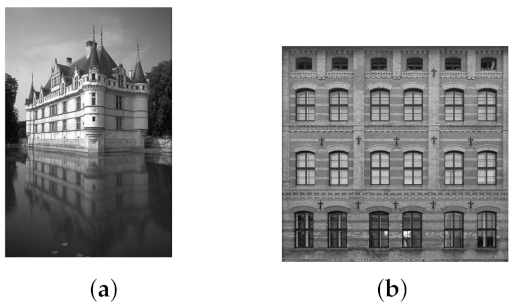
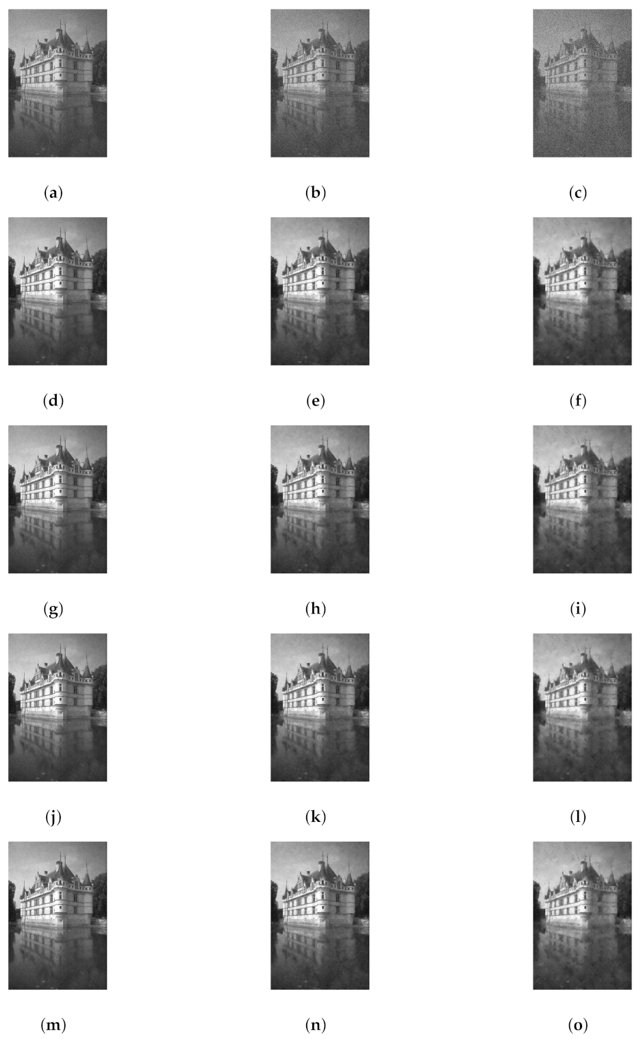
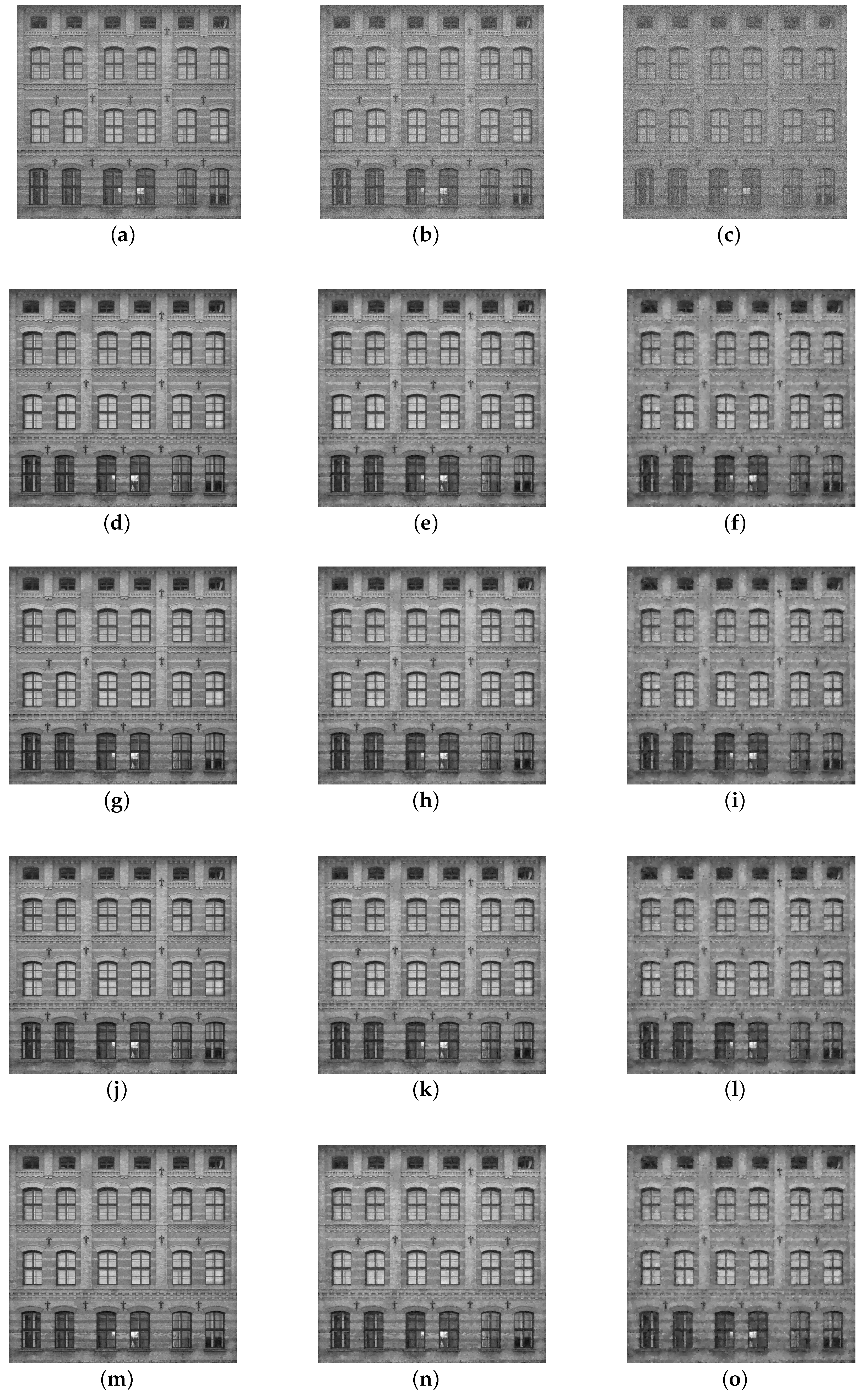
4. Numerical Experiments

In this section, we present some experimental results on image denoising problems under Gaussian noise. We compare the proposed algorithms with the FB_BH algorithm (5) and the FBF_BH algorithm (8). We call Algorithm 1 the FB algorithm. On the other hand, we refer to the proposed Algorithm 2 as the FBHF algorithm. All numerical experiments were implemented on Matlab R2016b on a Lenovo laptop with Intel i7-6700 CPU 3.40 GHz and 4 GB memory.

4.1. Image Denoising Problems

In this subsection, we show how the proposed algorithms could be applied to solve image denoising problems.

Let $b\in {\mathbb{R}}^n$ be the observed and vectorized noisy image of size $M\times N$ (with $n=MN$ for greyscale and $n=3MN$ for colored images). Let $k\ge 1$, and define

$$D_k:=\left[\begin{array}{cccccc}\hfill -1& \hfill 1& \hfill 0& \hfill 0& \hfill \cdots & \hfill 0\\ \hfill 0& \hfill -1& \hfill 1& \hfill 0& \hfill \cdots & \hfill 0\\ \hfill ⋮& \hfill & \hfill \ddots & \hfill \ddots & \hfill & \hfill ⋮\\ \hfill 0& \hfill \cdots & \hfill 0& \hfill -1& \hfill 1& \hfill 0\\ \hfill 0& \hfill \cdots & \hfill 0& \hfill 0& \hfill -1& \hfill 1\\ \hfill 0& \hfill \cdots & \hfill 0& \hfill 0& \hfill 0& \hfill 0\end{array}\right]\in {\mathbb{R}}^{k\times k},$$

(44)

which models the discrete first-order derivative. We denote by $A\otimes B$ the Kronecker product of the matrices A and B and define

$$D_x=I_N\otimes D_M,D_y=D_N\otimes I_M\mathrm{and}{\mathcal{D}}_1=\left[\begin{array}{c}{D}_x\\ D_y\end{array}\right]$$

(45)

where $D_x$ and $D_y$ represent the vertical and horizontal difference operators, respectively, and $I_N$ and $I_M$ are the identity matrices of sizes N and M, respectively. Further, we define the discrete second-order derivatives matrices

$$D_{xx}=I_N\otimes \left(-D_M^T{D}_M\right),D_{yy}=\left(-D_N^T{D}_N\right)\otimes I_M,{\mathcal{D}}_2=\left[\begin{array}{c}{D}_{xx}\hfill \\ D_{yy}\hfill \end{array}\right],$$

(46)

and

$$L_1=\left[\begin{array}{cc}-D_x^T& 0\\ 0& -D_y^T\end{array}\right].$$

(47)

We mainly consider the following two constrained image denoising models:

$$\left({\ell }_2-\mathrm{IC}\right)\underset{x\in C}{min}\left\{\frac{1}{2}{\parallel x-b\parallel }^2+\left(\left({\alpha }_1{\parallel ·\parallel }_1\circ {\mathcal{D}}_1\right)\square \left({\alpha }_2{\parallel ·\parallel }_1\circ {\mathcal{D}}_2\right)\right)\left(x\right)\right\},$$

(48)

and

$$\left({\ell }_2-\mathrm{MIC}\right)\underset{x\in C}{min}\left\{\frac{1}{2}{\parallel x-b\parallel }^2+\left(\left({\alpha }_1{\parallel ·\parallel }_1\right)\square \left({\alpha }_2{\parallel ·\parallel }_1\circ L_1\right)\right)\left({\mathcal{D}}_{1}x\right)\right\},$$

(49)

where ${\alpha }_1>0,{\alpha }_2>0$ are the regularization parameters, and C is a nonempty closed convex set. By using the indicator function, both of the constrained ${\ell }_2-\mathrm{IC}$ and ${\ell }_2^2-\mathrm{MIC}$ can be reformulated as the following unconstrained optimization problem,

$$\left({\ell }_2-\mathrm{IC}\right)\underset{x\in R^n}{min}\left\{\frac{1}{2}{\parallel x-b\parallel }^2+\left(\left({\alpha }_1{\parallel ·\parallel }_1\circ {\mathcal{D}}_1\right)\square \left({\alpha }_2{\parallel ·\parallel }_1\circ {\mathcal{D}}_2\right)\right)\left(x\right)+{\delta }_C\left(x\right)\right\},$$

(50)

and

$$\left({\ell }_2-\mathrm{MIC}\right)\underset{x\in R^n}{min}\left\{\frac{1}{2}{\parallel x-b\parallel }^2+\left(\left({\alpha }_1{\parallel ·\parallel }_1\right)\square \left({\alpha }_2{\parallel ·\parallel }_1\circ L_1\right)\right)\left({\mathcal{D}}_{1}x\right)+{\delta }_C\left(x\right)\right\}.$$

(51)

It is easy to see that (50) and (51) are special cases of the general convex minimization problem (36), respectively. In fact, let $m=1$, $z=0$, and $r_1=0$. For the ${\ell }_2-\mathrm{IC}$, let $f\left(x\right)={\delta }_C\left(x\right)$, $g_1\left(x\right)={\alpha }_1{\parallel x\parallel }_1$, $l_1\left(x\right)={\alpha }_2{\parallel x\parallel }_1$, $K_1={\mathcal{D}}_1$, $M_1={\mathcal{D}}_2$, $L_1=I$, and $h\left(x\right)=\frac{1}{2}{\parallel x-b\parallel }^2$; for the ${\ell }_2-\mathrm{MIC}$, let $f\left(x\right)={\delta }_C\left(x\right)$, $g_1\left(x\right)={\alpha }_1{\parallel x\parallel }_1$, $l_1\left(x\right)={\alpha }_2{\parallel x\parallel }_1$, $K_1=I$, $M_1=L_1$, $L_1={\mathcal{D}}_1$, and $h\left(x\right)=\frac{1}{2}{\parallel x-b\parallel }^2$.

4.2. Numerical Settings

The test images are shown in Figure 1. In our experiments, the test image is added by Gaussian noise with zero mean and standard deviation ${\sigma }_g$. In the following experiment, we set $C=\{x\in R^n|0\le x_i\le 255\}$.

We use the peak-signal-to-noise (PSNR) and the structural similarity index (SSIM) [24] to evaluate the quality of the restored images, which are defined by

$$PSNR=20{log}_{10}\frac{255\sqrt{mn}}{\parallel x-\tilde{x}\parallel },$$

and

$$SSIM=\frac{(2{\mu }_1{\mu }_2+c_1)(2{\sigma }_{12}+c_2)}{(2{\mu }_1^2{\mu }_2^2+c_1)({\sigma }_1^2+{\sigma }_2^2+c_2)},$$

where $x\in R^n$ is the original image, $\tilde{x}\in R^n$ is the restored image, $c_1>0$ and $c_2>0$ are small constants, ${\mu }_1$ and ${\mu }_2$ are the mean values of x and $\tilde{x}$, respectively; ${\sigma }_1$ and ${\sigma }_2$ are the variances of x and $\tilde{x}$, respectively; and ${\sigma }_{12}$ is the covariance of x and $\tilde{x}$.

The criterion for stopping all algorithms is that the relative error of two consecutive iterations satisfies the following inequality

$$\frac{\parallel x_{n+1}-x_n\parallel }{\parallel x_n\parallel }<\epsilon ,$$

where $\epsilon >0$ is a given small constant.

We tune the regularization parameters ${\alpha }_1$ and ${\alpha }_2$ so as to maximize the PSNR values of the restored images. The choices of ${\alpha }_1$ and ${\alpha }_2$ are presented in

Table 1. The regularization parameters selection of the ${\ell }_2-\mathrm{IC}$ and ${\ell }_2-\mathrm{MIC}$.

Image	Model	$\mathit{\sigma }=\mathbf{15}$		$\mathit{\sigma }=\mathbf{25}$		$\mathit{\sigma }=\mathbf{50}$
		${\mathit{\alpha }}_{\mathbf{1}}$	${\mathit{\alpha }}_{\mathbf{2}}$	${\mathit{\alpha }}_{\mathbf{1}}$	${\mathit{\alpha }}_{\mathbf{2}}$	${\mathit{\alpha }}_{\mathbf{1}}$	${\mathit{\alpha }}_{\mathbf{2}}$
Castle	${\ell }_2-\mathrm{IC}$	7.7	21.2	14.7	29.7	35.5	123.9
	${\ell }_2-\mathrm{MIC}$	7.6	21.1	14.8	50.8	35.7	115.9
Building	${\ell }_2-\mathrm{IC}$	6.1	25.3	12.4	33	31.3	87.8
	${\ell }_2-\mathrm{MIC}$	6.1	27.8	12.5	49.4	31.8	140

.

4.3. Numerical Results and Discussion

In the first experiment, we discuss the influence of the selection of iterative parameters on the convergence speed of the compared algorithms. According to the convergence theorems, the parameter selection of these algorithms is shown in

Table 2. The parameter selection of the compared algorithms.

Model	Method	Parameter
${\ell }_2-\mathrm{IC}$	FB_BH	$\begin{array}{l}{\lambda }_n\in (0,1],2(1-\overline{\alpha })min\left\{\frac{1}{\tau },\frac{1}{{\theta }_1},\frac{1}{{\theta }_2},\frac{1}{{\gamma }_1},\frac{1}{{\gamma }_2},\frac{1}{\sigma }\right\}>1,\\ \overline{\alpha }=max\left\{\sqrt{\tau \sigma },2.8072\sqrt{{\theta }_1{\gamma }_1},5.6133\sqrt{{\theta }_2{\gamma }_2}\right\}\end{array}$
	FBF_BH	${\gamma }_n\in (0,0.1512)$
	FB	$\begin{array}{l}{\lambda }_n\in (0,2-\frac{1}{2\beta }),2\beta >1,(1-\overline{\alpha })min\left\{\frac{1}{\tau },\frac{1}{{\theta }_1},\frac{1}{{\theta }_2},\frac{1}{{\gamma }_1},\frac{1}{{\gamma }_2},\frac{1}{\sigma }\right\}>0,\\ \overline{\alpha }=max\left\{\sqrt{\tau \sigma },2.8072\sqrt{{\theta }_1{\gamma }_1},5.6133\sqrt{{\theta }_2{\gamma }_2}\right\},\beta =\frac{1}{\tau }-\sigma \end{array}$
	FBHF	${\gamma }_n\in (0,0.1704)$
${\ell }_2-\mathrm{MIC}$	FB_BH	$\begin{array}{l}{\lambda }_n\in (0,1],2(1-\overline{\alpha })min\left\{\frac{1}{\tau },\frac{1}{{\theta }_1},\frac{1}{{\theta }_2},\frac{1}{{\gamma }_1},\frac{1}{{\gamma }_2},\frac{1}{\sigma }\right\}>1,\\ \overline{\alpha }=max\left\{2.8072\sqrt{\tau \sigma },\sqrt{{\theta }_1{\gamma }_1},1.9926\sqrt{{\theta }_2{\gamma }_2}\right\}\end{array}$
	FBF_BH	${\gamma }_n\in (0,0.2627)$
	FB	$\begin{array}{l}{\lambda }_n\in (0,2-\frac{1}{2\beta }),2\beta >1,(1-\overline{\alpha })min\left\{\frac{1}{\tau },\frac{1}{{\theta }_1},\frac{1}{{\theta }_2},\frac{1}{{\gamma }_1},\frac{1}{{\gamma }_2},\frac{1}{\sigma }\right\}>0,\\ \overline{\alpha }=max\left\{2.8072\sqrt{\tau \sigma },\sqrt{{\theta }_1{\gamma }_1},1.9926\sqrt{{\theta }_2{\gamma }_2}\right\},\beta =\frac{1}{\tau }-7.8798\sigma \end{array}$
	FBHF	${\gamma }_n\in (0,0.3259)$

. For the ${\ell }_2-\mathrm{IC}$ and ${\ell }_2-\mathrm{MIC}$, let $h\left(x\right)=\frac{1}{2}{\parallel x-b\parallel }^2$, then, $\nabla h\left(x\right)=x-b$, and $\mu =1$.

We chose Castle in Figure 1 as the test image, and the Gaussian noise level ${\sigma }_g=15$. The numerical results of the FBF_BH algorithm and the FBHF algorithm with a different selections of the parameters $\left\{{\gamma }_n\right\}$ are reported in

Table 3. Numerical results of the FBF_BH algorithm and the FBHF algorithm with different selections of parameters in terms of the PSNR, SSIM, and number of iterations (Iter).

Method	Model	${\mathit{\gamma }}_{\mathit{n}}$	$\mathit{\epsilon }={10}^{-5}$			$\mathit{\epsilon }={10}^{-6}$
			PSNR	SSIM	Iter	PSNR	SSIM	Iter
FBF_BH	${\ell }_2-\mathrm{IC}$	0.03	30.5138	0.8410	1791	30.5346	0.8409	6572
		0.05	30.5225	0.8410	1411	30.5356	0.8409	5203
		0.07	30.5287	0.8410	1227	30.5361	0.8409	4445
		0.09	30.5309	0.8410	1103	30.5370	0.8409	3994
		0.11	30.5317	0.8410	1003	30.5379	0.8409	3730
		0.13	30.5323	0.8410	946	30.5386	0.8409	3560
		0.15	30.5330	0.8410	888	30.5391	0.8409	3372
	${\ell }_2-\mathrm{MIC}$	0.03	30.5330	0.8384	2287	30.5434	0.8391	4984
		0.07	30.5358	0.8386	1126	30.5451	0.8392	2824
		0.11	30.5378	0.8387	796	30.5460	0.8393	2207
		0.15	30.5390	0.8388	634	30.5365	0.8393	1896
		0.19	30.5400	0.8388	538	30.5467	0.8393	1686
		0.23	30.5409	0.8389	474	30.5468	0.8393	1518
		0.26	30.5414	0.8389	439	30.5470	0.8393	1456
FBHF	${\ell }_2-\mathrm{IC}$	0.03	30.5138	0.8410	1790	30.5346	0.8409	6474
		0.05	30.5225	0.8410	1411	30.5356	0.8409	5203
		0.07	30.5287	0.8410	1227	30.5361	0.8409	4449
		0.09	30.5309	0.8410	1103	30.5370	0.8409	3994
		0.11	30.5317	0.8410	1003	30.5379	0.8409	3729
		0.13	30.5323	0.8410	946	30.5386	0.8409	3561
		0.15	30.5330	0.8410	887	30.5391	0.8409	3371
		0.17	30.5336	0.8410	837	30.5393	0.8409	3169
	${\ell }_2-\mathrm{MIC}$	0.03	30.5330	0.8384	2286	30.5434	0.8391	4983
		0.07	30.5358	0.8386	1126	30.5452	0.8392	2824
		0.11	30.5378	0.8387	796	30.5460	0.8393	2207
		0.15	30.5390	0.8388	633	30.5465	0.8393	1896
		0.19	30.5401	0.8388	538	30.5467	0.8393	1686
		0.23	30.5410	0.8389	474	30.5468	0.8393	1519
		0.27	30.5416	0.8389	428	30.5470	0.8393	1432
		0.31	30.5421	0.8390	394	30.5471	0.8394	1346
		0.32	30.5422	0.8390	387	30.5471	0.8394	1317

. It can be seen from Table 3 that both the FBF_BH algorithm and the FBHF algorithm gradually reduced the number of iterations as the step size parameter increased.

For the FB_BH algorithm and the FB algorithm, we selected several combinations of the parameters in

Table 4. Parameter selection of the FB_BH algorithm and the FB algorithm.

Method	Model	Case	${\mathit{\theta }}_{\mathbf{1}}$	${\mathit{\theta }}_{\mathbf{2}}$	${\mathit{\gamma }}_{\mathbf{1}}$	${\mathit{\gamma }}_{\mathbf{2}}$	$\mathit{\tau }$	$\mathit{\sigma }$	${\mathit{\lambda }}_{\mathit{n}}$
FB_BH	${\ell }_2-\mathrm{IC}$	1	0.3	0.15	0.3	0.15	0.3	0.3	1
		2	0.2	0.15	0.2	0.15	0.3	0.3	1
		3	0.2	0.1	0.2	0.1	0.2	0.2	1
		4	0.2	0.2	0.2	0.1	0.1	0.3	1
	${\ell }_2-\mathrm{MIC}$	1	0.3	0.15	0.3	0.15	0.3	0.3	1
		2	0.4	0.2	0.3	0.1	0.2	0.3	1
		3	0.1	0.2	0.1	0.2	0.3	0.2	1
		4	0.1	0.1	0.1	0.1	0.2	0.4	1
FB	${\ell }_2-\mathrm{IC}$	1	0.3	0.15	0.3	0.15	0.3	0.3	1.4
		2	0.2	0.1	0.3	0.2	0.3	0.4	1.5
		3	0.3	0.2	0.3	0.1	0.2	0.2	1.8
		4	0.2	0.2	0.2	0.1	0.1	0.3	1.3
	${\ell }_2-\mathrm{MIC}$	1	0.5	0.4	0.5	0.4	0.3	0.3	1.4
		2	0.4	0.3	0.4	0.4	0.25	0.25	1.5
		3	0.3	0.2	0.3	0.2	0.2	0.2	1.8
		4	0.2	0.3	0.2	0.3	0.3	0.3	1.4

.

According to the iteration parameters in Table 4, the obtained numerical results are shown in

Table 5. Numerical results of the FB_BH algorithm and the FB algorithm with different parameters in terms of the PSNR, SSIM, and number of iterations (Iter).

Method	Model	Case	$\mathit{\epsilon }={\mathbf{10}}^{\mathbf{-}\mathbf{5}}$			$\mathit{\epsilon }={\mathbf{10}}^{\mathbf{-}\mathbf{6}}$
			PSNR	SSIM	Iter	PSNR	SSIM	Iter
FB_BH	${\ell }_2-\mathrm{IC}$	1	30.5386	0.8411	753	30.5405	0.8409	2846
		2	30.5361	0.8411	824	30.5399	0.8409	3117
		3	30.5379	0.8411	885	30.5397	0.8409	3277
		4	30.5369	0.8409	818	30.5395	0.8408	3087
	${\ell }_2-\mathrm{MIC}$	1	30.5386	0.8411	657	30.5411	0.8409	2481
		2	30.5412	0.8389	534	30.5468	0.8393	1632
		3	30.5253	0.8408	930	30.5364	0.8409	3603
		4	30.5313	0.8410	1034	30.5375	0.8309	3875
FB	${\ell }_2-\mathrm{IC}$	1	30.5387	0.8411	701	30.5408	0.8409	2640
		2	30.5382	0.8412	754	30.5419	0.8410	2514
		3	30.5389	0.8409	601	30.5407	0.8409	2242
		4	30.5377	0.8409	735	30.5398	0.8408	2725
	${\ell }_2-\mathrm{MIC}$	1	30.5442	0.8391	292	30.5475	0.8394	1047
		2	30.5435	0.8391	321	30.5474	0.8394	1140
		3	30.5447	0.8392	285	30.5476	0.8394	980
		4	30.5435	0.8391	372	30.5474	0.8394	1121

.

According to the results of Table 3 and Table 5, we chose the following parameters of the compared algorithms for the following experiments.

(1) For the FBF_BH algorithm, the best parameter of ${\ell }_2-\mathrm{IC}$ was ${\gamma }_n=0.15$, and the best parameter of ${\ell }_2-\mathrm{MIC}$ was ${\gamma }_n=0.26$.

(2) For the FBHF algorithm, the best parameter of ${\ell }_2-\mathrm{IC}$ was ${\gamma }_n=0.17$, and the best parameter of ${\ell }_2-\mathrm{MIC}$ was ${\gamma }_n=0.32$.

(3) For the FB_BH algorithm, the best parameters of ${\ell }_2-\mathrm{IC}$ were ${\theta }_1=0.3,{\gamma }_1=0.3,{\theta }_2=0.15,{\gamma }_2=0.15,{\lambda }_n=1,\tau =0.3,$ and $\sigma =0.3$, and the best parameters of ${\ell }_2-\mathrm{MIC}$ were ${\theta }_1=0.4,{\gamma }_1=0.3,{\theta }_2=0.2,{\gamma }_2=0.2,{\lambda }_n=1,\tau =0.2,$ and $\sigma =0.3$.

(4) For the FB algorithm, the best parameters of ${\ell }_2-\mathrm{IC}$ were ${\theta }_1=0.3,{\gamma }_1=0.3,{\theta }_2=0.2,{\gamma }_2=0.1,{\lambda }_n=1.8,\tau =0.2,$ and $\sigma =0.2$, and the best parameters of ${\ell }_2-\mathrm{MIC}$ were ${\theta }_1=0.3,{\gamma }_1=0.3,{\theta }_2=0.2,{\gamma }_2=0.2,{\lambda }_n=1.8,\tau =0.2,$ and $\sigma =0.2$.

In the second experiment, we tested the performance of the compared algorithms for solving ${\ell }_2-\mathrm{IC}$ and ${\ell }_2-\mathrm{MIC}$. We present the numerical results by each algorithm in

Table 6. Numerical results of the compared algorithms in terms of the PSNR, SSIM, and number of iterations (Iter).

Image	Model	${\mathit{\sigma }}_{\mathit{g}}$	FBF_BH			FBHF
			PSNR	SSIM	Iter	PSNR	SSIM	Iter
Castle	${\ell }_2-\mathrm{IC}$	15	30.5330	0.8410	888	30.5336	0.8410	837
		25	27.9370	0.7799	786	27.9376	0.7798	736
		50	24.9407	0.7027	1364	24.9427	0.7026	1315
	${\ell }_2-\mathrm{MIC}$	15	30.5414	0.8389	439	30.5422	0.8390	387
		25	27.9352	0.7796	665	27.9379	0.7798	615
		50	24.9332	0.7010	1169	24.9380	0.7014	1093
Building	${\ell }_2-\mathrm{IC}$	15	28.3617	0.8404	1365	28.3612	0.8404	1339
		25	25.5939	0.7333	1020	25.5943	0.7333	971
		50	22.6506	0.5558	1100	22.6510	0.5558	1045
	${\ell }_2-\mathrm{MIC}$	15	28.3663	0.8405	492	28.3665	0.8405	431
		25	25.5997	0.7332	623	25.6001	0.7332	570
		50	22.6716	0.5565	1146	22.6724	0.5565	1070
Image	Model	${\mathit{\sigma }}_{\mathit{g}}$	FB_BH			FB
			PSNR	SSIM	Iter	PSNR	SSIM	Iter
Castle	${\ell }_2-\mathrm{IC}$	15	30.5386	0.8411	753	30.5389	0.8409	601
		25	27.9398	0.7799	691	27.9452	0.7797	548
		50	24.9415	0.7027	1321	24.9485	0.7013	1039
	${\ell }_2-\mathrm{MIC}$	15	30.5412	0.8389	534	30.5426	0.8391	398
		25	27.9330	0.7795	734	27.9400	0.7799	601
		50	24.9278	0.7707	1243	24.9418	0.7017	1085
Building	${\ell }_2-\mathrm{IC}$	15	28.3635	0.8405	1047	28.3634	0.8404	906
		25	25.5952	0.7333	832	25.5956	0.7334	719
		50	22.6051	0.5563	1018	22.6521	0.5564	849
	${\ell }_2-\mathrm{MIC}$	15	28.3664	0.8405	623	28.3668	0.8405	420
		25	25.5822	0.7329	584	25.6005	0.7322	554
		50	22.6629	0.5577	1043	22.6653	0.5578	856

.

From the experimental results of Table 6, we can see that the proposed FBHF algorithm converged faster than the FBF_BH algorithm in terms of the number of iterations while ensuring higher PSNR and SSIM values. Meanwhile, the proposed FB algorithm also converged faster than the FB_BH algorithm. The obtained results verify that the proposed algorithms are better than those in [4]. Some of the recovered images are shown in Figure 2 and Figure 3, respectively.

5. Conclusions

In this paper, we studied the convergence of two different primal-dual splitting algorithms for solving monotone inclusions (3) and (4). Firstly, we proved the convergence of the forward–backward type algorithm (5). Our parameter conditions improved the results of Boţ and Hendrich [4]. Secondly, we proposed a new forward–backward–half-forward type algorithm (32). In contrast to the forward–backward–forward type algorithm (8), the iterative sequences in the proposed forward–backward–half-forward type algorithm (32) used the cocoercive operator only once via the forward step. Finally, we applied the proposed algorithms to solve image denoising problems (48) and (49). The numerical results demonstrated the advantages of the proposed algorithms.

References

1. Vũ, B.C. A splitting algorithm for dual monotone inclusions involving cocoercive operators. Adv. Comput. Math. 2013, 38, 667–681. [Google Scholar] [CrossRef]
2. Pesquet, J.-C.; Repetti, A. A class of randomized primal-dual algorithms for distributed optimization. J. Nonlinear Convex Anal. 2015, 16, 2453–2490. [Google Scholar]
3. Vũ, B.C. A spliting algorithm for coupled system of primal-dual monotone inclusions. J. Optim. Theory Appl. 2015, 164, 993–1025. [Google Scholar] [CrossRef]
4. Boţ, R.I.; Hendrich, C. Solving monotone inclusions involving parallel sums of linearly composed maximally monotone operators. Inverse Probl. Imaging 2016, 10, 617–640. [Google Scholar] [CrossRef] [Green Version]
5. Boţ, R.I.; Hendrich, C. A douglas-rachford type primal-dual method for solving inclusions with mixtures of composite and parallel-sum type monotone operators. SIAM J. Optim. 2013, 4, 2541–2565. [Google Scholar] [CrossRef] [Green Version]
6. Boţ, R.I.; Csetnek, E.R.; Heinrich, A. A primal-dual splitting for finding zeros of sums of maximal monotone operators. SIAM J. Optim. 2013, 23, 2011–2036. [Google Scholar] [CrossRef]
7. Yang, Y.X.; Tang, Y.C.; Wen, M.; Zeng, T.Y. Preconditioned douglas-rachford type primal-dual method for solving composite monotone inclusion problems with applications. Inverse Probl. Imaging 2021, 15, 787–825. [Google Scholar] [CrossRef]
8. Briceño-Arias, L.M.; Combettes, P.L. A monotone+skew splitting splitting model for composite monotone inclusions in duality. SIAM J. Control Optim. 2011, 21, 1230–1250. [Google Scholar] [CrossRef] [Green Version]
9. Combettes, P.L.; Pesquet, J.-C. Primal-dual splitting algorithm for solving inclusions with mixtures of composite, lipschitzian, and paralle-sum type monotone operators. Set-Valued Var. Anal. 2012, 20, 307–330. [Google Scholar] [CrossRef] [Green Version]
10. Combettes, P.L. Systems of structured monotone inclusions: Duality, algorithms, and applications. SIAM J. Optim. 2013, 23, 2420–2447. [Google Scholar] [CrossRef] [Green Version]
11. Becker, S.R.; Combettes, P.L. An algorithm for splitting parallel sums of linearly composed monotone operatos with applications to signal recovery. J. Nonlinear Convex Anal. 2014, 15, 137–159. [Google Scholar]
12. Boţ, R.I.; Hendrich, C. Convergence analysis for a primal-dual monotone+skew splitting algorithm with applications to total variation minimization. J. Math. Imaging Vis. 2014, 49, 551–568. [Google Scholar]
13. Alotaibi, A.; Combettes, P.L.; Shahzad, N. Solving coupled composite monotone inclusions by successive fejér approximations of their kukn-tucker set. SIAM J. Optim. 2014, 24, 2076–2095. [Google Scholar] [CrossRef] [Green Version]
14. Tran-Dinh, Q.; Vu, B.C. A new splitting method for solving composite monotone inclusions involving parallel-sum operators. arXiv 2015, arXiv:1505.07946. [Google Scholar]
15. Combettes, P.L.; Eckstein, J. Asynchronous block-iterative primal-dual decomposition methods for monotone inclusions. Math. Program. 2018, 168, 645–672. [Google Scholar] [CrossRef] [Green Version]
16. Bardaro, C.; Bevignani, G.; Mantellini, I.; Seracini, M. Bivariate generalized exponential sampling series and applications to seismic waves. Constr. Math. Anal. 2019, 2, 153–167. [Google Scholar] [CrossRef]
17. Johnstone, P.R.; Eckstein, J. Projective splitting with forward steps. Math. Program. 2020, 1–40. [Google Scholar] [CrossRef]
18. Chambolle, A.; Lions, P.L. Image recovery via total variation minimizaing and related problems. Numer. Math. 1997, 76, 167–188. [Google Scholar] [CrossRef]
19. Setzer, S.; Steidl, G.; Teuber, T. Infimal convolution regularization with discrete l1-type functionals. Commun. Math. Sci. 2011, 9, 797–827. [Google Scholar] [CrossRef] [Green Version]
20. Combettes, P.L.; Vũ, B.C. Variable metric forward-backward splitting with applications to monotone inclusions in duality. Optimization 2014, 63, 1289–1318. [Google Scholar] [CrossRef] [Green Version]
21. Tseng, P. A modified forward-backward splitting method for maximal monotone mappings. SIAM J. Control Optim. 2000, 38, 431–446. [Google Scholar] [CrossRef]
22. Briceño-Arias, L.M.; Davis, D. Forward-backward-half forward algorithm for solving monotone inclusions. SIAM J. Optim. 2018, 28, 2839–2871. [Google Scholar] [CrossRef] [Green Version]
23. Bauschke, H.H.; Combettes, P.L. Convex Analysis and Monotone Operator Theory in Hilbert Spaces, 2nd ed.; Springer: London, UK, 2017. [Google Scholar]
24. Wang, Z.; Bovik, A.C.; Sheikh, H.R.; Simoncelli, E.P. Image quality assessment: From error visibility to structural similarity. IEEE Trans. Image Process. 2004, 13, 600–612. [Google Scholar] [CrossRef] [PubMed] [Green Version]
Figure 1. Test images. (a) 481 × 321 “Castle” image, (b) 493 × 517 “Building” image.
Symmetry 13 02415 g001
Figure 2. Noisy and restored “Castle” images. (a) σ g = 15 . (b) σ g = 25 . (c) σ g = 50 . (d) 2 - IC /FBF_BH. (e) 2 - IC /FBF_BH. (f) 2 - IC /FBF_BH. (g) 2 - IC /FB_BH. (h) 2 - IC /FB_BH. (i) 2 - IC /FB_BH. (j) 2 - IC /FBHF. (k) 2 - IC /FBHF. (l) 2 - IC /FBHF. (m) 2 - IC /FB. (n) 2 - IC /FB. (o) 2 - IC /FB.
Symmetry 13 02415 g002
Figure 3. Noisy and restored “Building” images. (a) σ g = 15 . (b) σ g = 25 . (c) σ g = 50 . (d) 2 - IC /FBF_BH. (e) 2 - IC /FBF_BH. (f) 2 - IC /FBF_BH. (g) 2 - IC /FB_BH. (h) 2 - IC /FB_BH. (i) 2 - IC /FB_BH. (j) 2 - IC /FBHF. (k) 2 - IC /FBHF. (l) 2 - IC /FBHF. (m) 2 - IC /FB. (n) 2 - IC /FB. (o) 2 - IC /FB.
Symmetry 13 02415 g003