1. Introduction
Fractional calculus (FC) deals with the differentiation and integration of arbitrary order and it is used in the real world to model and analyze big problems. Fluid flow, electrical networks, fractals theory, control theory, electromagnetic theory, probability, statistics, optics, potential theory, biology, chemistry, diffusion, and viscoelasticity are just a few of the many fields where fractional calculus is used [
1,
2,
3,
4].
In recent years, fractional differential equations and integro-fractional differential equations (IFDEs) have captivated the hobby of many researchers in various fields of science and era due to the reality that realistic modeling of a bodily phenomenon with dependencies not only in the immediate time, but also in the past time history can be accomplished effectively using FC. However, in addition to modeling, the solution approaches and their dependability are crucial in detecting key points when a rapid divergence, convergence, or bifurcation begins. As a result, high-precision solutions are always required. Several strategies for solving fractional order differential equations were presented for this purpose (or integro-differential equations), [
1,
3,
4]. The Adomian decomposition method [
5], variational iteration method [
6], fractional differential transform method [
7], fractional difference method [
8], and power series method [
9] are the most commonly used ideas.
However, from the beginning of 1994, Laguerre, Legendre, Taylor, Fourier, Hermite, and Bessel polynomials have been employed in works [
10,
11,
12,
13,
14,
15] to solve linear differential, integral, and integro-differential difference equations and related systems. In addition, the Bessel polynomial of the first kind method has been used to find approximate solutions of differential, fractional differential equations, integro-differential equations of fractional order, LVIDEs, and LF-VIDEs [
16,
17,
18,
19].
The aim of this paper is to expand and apply the first kind of Bessel polynomial in matrix form, as well as the collocation techniques, to evaluate the approximate solution for the multi-high-order linear Fredholm–Volterra integro-fractional differential equations (FVIFDEs) of the general type:
together with mixed conditions:
where the fractional orders:
and
and
In addition,
is an unknown function, the functions
, and
are known, with constants
for all
,
are given.
3. Fundamental Matrix Relations
Recall Equation (1) and rewrite it as follows:
where
and the integral parts:
our purpose is to find a close approximation of Equation (1) in the
N-truncated Bessel series arrangement
So that are the unknown Bessel coefficients. Before we begin the approximate solution we must convert the solution and its in the parts to matrix form, within the mixed conditions of Equation (2).
3.1. Matrix Relation for the Fractional Derivative Part
To describe the solution
of Equation
, which is specified by the
-truncated Bessel series of Equation
. The function defined in relation
in a matrix form
or from Equation
The relationship between the matrix
and its derivative
is also written as follows:
where
We will also get the recurrence relations from Equation (8):
Here, note that
is an identity matrix of dimension
. Using mathematical induction, we can prove that Equation (9) is correct. By applying the same concept to Equation (7) and using Equation (9), we attain matrix relation
By using Equation (7) with (9) and applying the Caputo Definition 4, with Lemma 1 and 2, we can convert the fractional terms
that is
for all
to matrix form:
Since
Thus, for all
in general we obtain
and
Using mathematical induction, we can prove that Equations (12) and (13) are correct. By substituting expressions
and
into
, As well we can make this assumption
, we have
3.2. Matrix Relation for the Fredholm Integral Part
The
-truncated Taylor series around (0,0), [
27] and the
-truncated Bessel series can be used to approximate the Fredholm kernel functions
, respectively
where
In matrix forms, the Equation (15) may be written as Equations (16) and (17), respectively
and
From Equations (16) and (17), it also comes out according to Equation (3), the following relation
In the same way from Equations (12) and (13), convert
by apply the Caputo Definition 4 with Lemma 1 to the matrix form, we obtain
where
is defined at Equation (11). We obtain the matrix relation (20), put the Equation (3) into (17), and then replace the obtained matrix with matrix (19) in the Fredholm integral part
in Equation (4)
where
We can get the last matrix form (21) by replacing the matrix relation (18) into expression (20).
3.3. Matrix Relation for the Volterra Integral Part
The
-truncated Taylor series around (0,0), [
27] and the
-truncated Bessel series can be used to approximate the Volterra kernel functions
, respectively
where
The relations in Equation (22) can be transformed into matrix forms:
and
from Equations (23) and (24), it also comes out according to Equation (3) we obtain the following relation:
Finally, in the same way from Equations (12) and (13), convert
, by applying the Caputo Definition 4 with Lemma 1, 2 and 3 to matrix form, we obtain
where
define at Equation (11). We obtain the matrix relation (27), put the Equation (3) into (24) and then replace the obtained matrix with matrix (26) in Fredholm integral part
in Equation (4)
where
We can get the last matrix form (28) by replacing the matrix relation (25) into expression (27).
3.4. Matrix Relation for the Conditions
For each
and
applying the relation (10) to each mixed condition of Equation (2), we obtain the corresponding condition matrix forms as follows.
4. Method of Solution
To construct the fundamental matrix equation that corresponds to Equation (1), insert the matrix relations (14), (21), and (28) into Equation (4) to obtain the following matrix equation
We get the following system of equations by setting the collocation points, [
28], described by
:
or in brief, the most important matrix equation is
where
for all
are the unit matrix,
also, for each fractional order
we are putting
where
where, respectively
For all . In Equation (31) we have explained that their dimensions are similar to those of . Moreover, in Equation (31), these matrices are written in full, their measured dimensions can be observed by , and respectively.
As a result, the fundamental matrix Equation (31) that corresponds to Equation (1) may be expressed as
where
Note that, Equation (32) is a set of
linear algebraic equations with unknown Bessel coefficients
The matrix form (29) for the conditions, on the other hand, may be represented as
Hence, we may solve Equation (1) under mixed conditions (2) by substituting the rows of the matrices
and
for the rows of the matrices
respectively.
The new augmented matrix (some time may be symmetry) of the preceding system is as follows if the last
-rows of the matrix (32) are replaced for simplicity:
Take note that rank If it isn’t, the suggested technique fails to offer a solution; but in this case, in this situation, the number of collocation points (or, equivalently, the dimension of the matrix ) can be increased to get the specific or general answer. As a result, we may write , and therefore the elements are uniquely determined.
Moreover, select that we define needs to be greater than , i.e., If it is not, the proposed strategy is thus unable to give a solution, because matrix becomes a zero matrix, we only get zero solution.
5. Numerical Examples
In this work, we choose several examples where the exact solution already exists to demonstrate the accuracy. They were all carried out on a computer using a Python program V3.8.8 (2021). The least square errors (L.S.E) in tables are the values of at -selected collocation points and the running time is also provided in tabular form.
Example 1. Consider the linear Fredholm–Volterra integro-differential equation of multi-higher fractional order, given by where
with the boundary conditions
which is the exact solution
Let us now determine the
-truncated Bessel series approximate solution
Here, from the considered, example we have:
Hence
so take, the collocation point sets are
and the fundamental matrix equation of the given (LF-VFIDEs) is derived from Equation (31), written as
where
putting all above matrices in matrix Equation (32) and calculating it, this fundamental matrix equation’s augmented matrix is:
For our consider example, the boundary conditions from Equation (33) have the following matrix forms:
or clearly
The new augmented matrix depending on conditions is constructed as follows from the system (34):
The Bessel coefficient matrix
is obtained by solving this system.
hence, for
the approximate solution of the problem is formed as
for
and
, similarly as steps above and running the general python program which are written for this purpose we obtain the approximate solution of the problem, respectively.
and
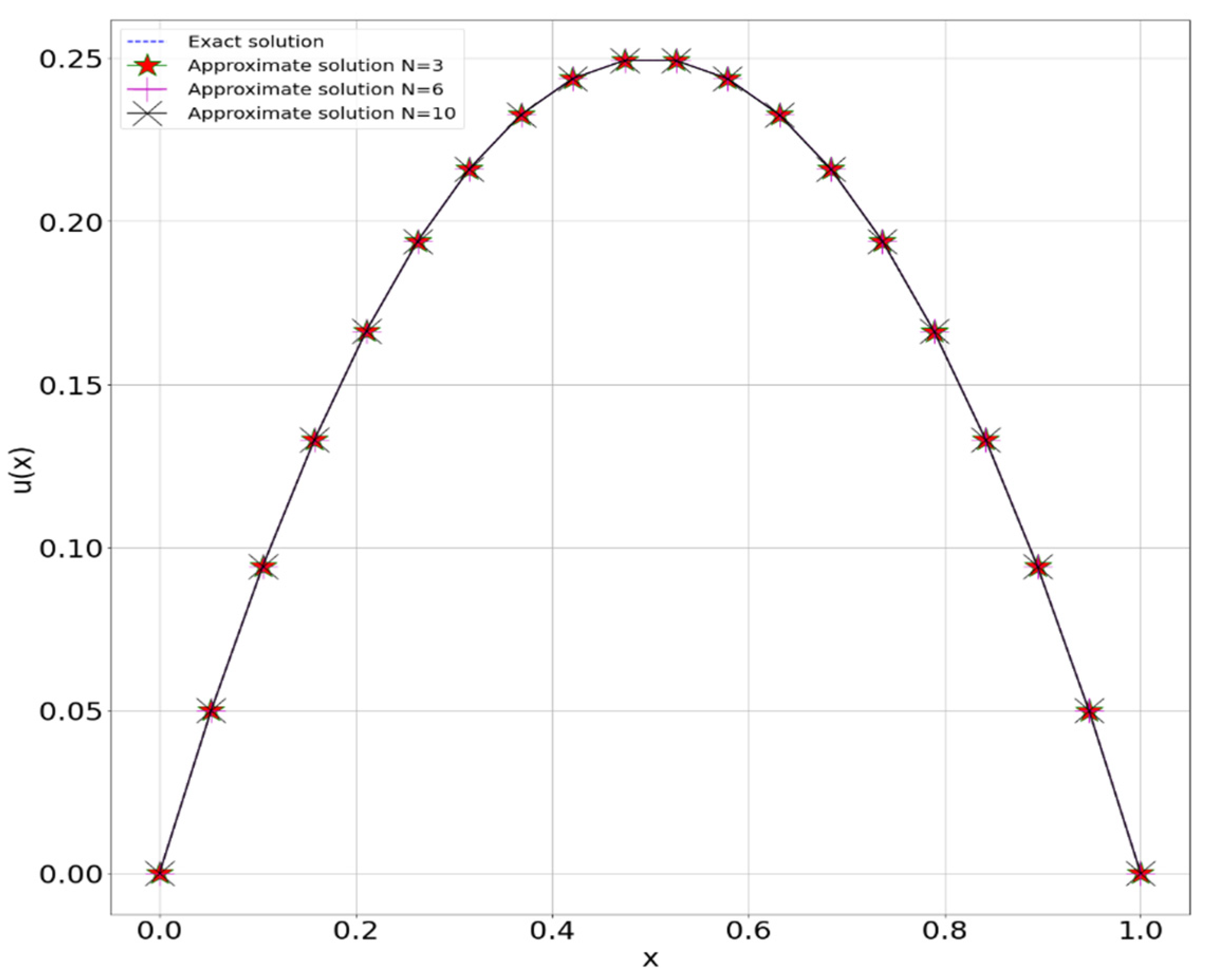
In
Table 1, Comparison the exact solution
with the approximate solution
of Example 1 for
, respectively, in terms of least square error and running time.
Example 2. Let us now consider the LF-VIFDEs on the closed bounded interval given by where
with the boundary conditions:
The exact solution is
Let us now calculate the coefficients
of approximate solution with the aid of the truncated Bessel series:
Here, from the considered example we have:
Hence
so take
, the set of collocation points, and the fundamental matrix equation of the given (LF-VFIDEs) is derived from Equation (31), written as
After inputting each of the parameters above by running the general python program, which are written for this purpose for
, we obtain the approximate solution of the problem,
Similarly, the approximate solution of the problem for
respectively, we obtain
and
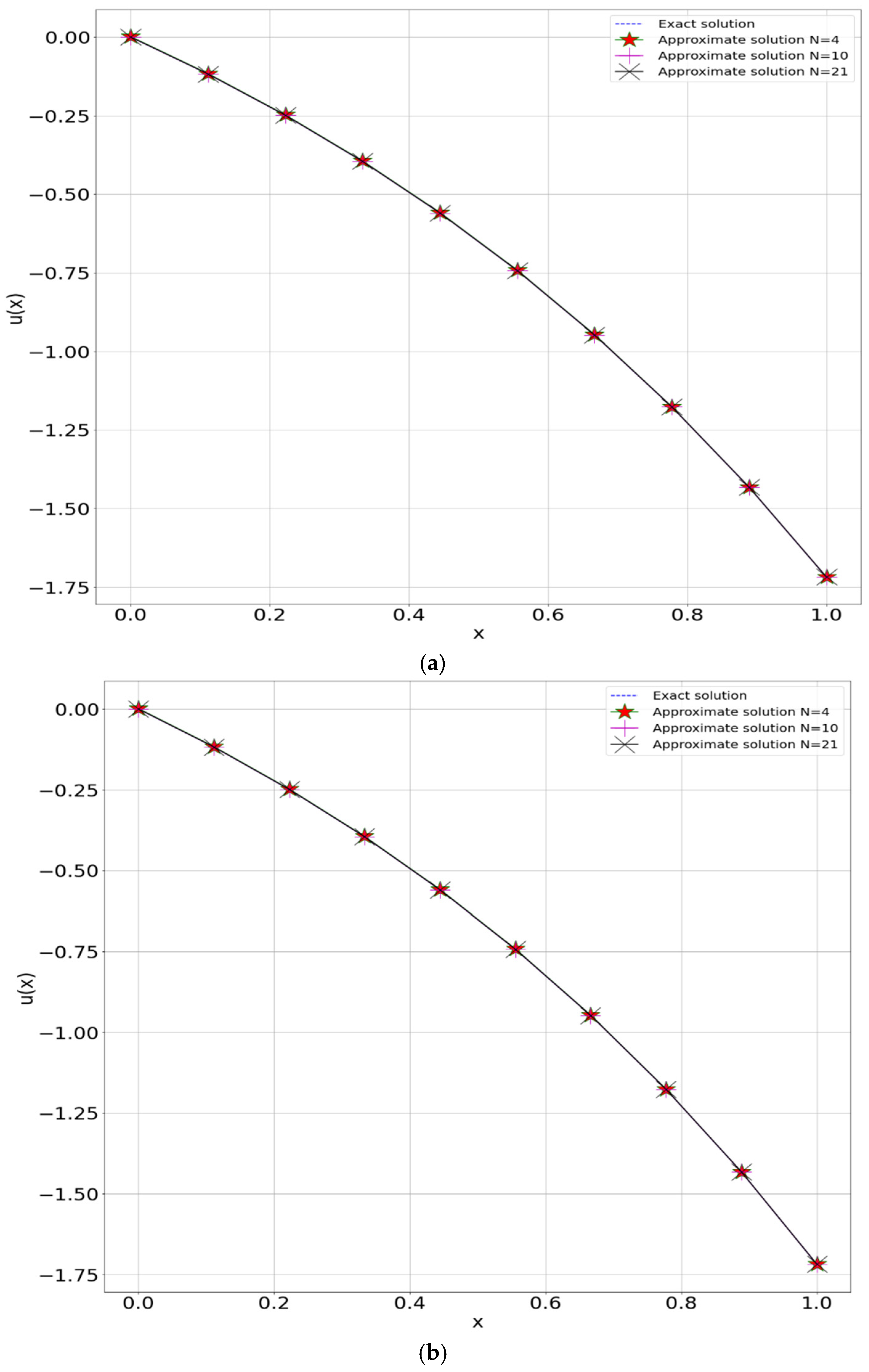
In
Table 2 comparison in terms of least square error and running time the exact solution
with the approximate solution
of example 2 for
, respectively.
Figure 1 and
Figure 2 illustrate a comparison between the exact solution and approximate solution of LF-VIFDEs of Examples 1 and 2, respectively. To show the result of the proposed method to an exact solution, we present
Table 1 and
Table 2, respectively. Each of the plots is drawn with our Python program version 3.8.8 (2021).
Example 3. Let us consider the linear Fredholm–Volterra fractional integro-differential equation on the closed bounded interval [0,1]:
where
with the boundary conditions
which is the exact solution
Let us now calculate the coefficients
of approximate solution with the aid of the truncated Bessel series:
Here, from consider example we have:
Suppose that, we take
terms from the homogeneous part
:
Hence
, the fundamental matrix equation of the given (LF-VFIDEs) is derived from Equation (31), written as
We choose if
, the approximate solution of the problem for
respectively
and
we choose if
the approximate solution of the problem for
respectively
and
Similarly doing it for
, the approximate solution of the problem for
respectively
and
In
Table 3 presents a comparison between the exact solution
and approximate solution
, when we choose
respectively. For each of them we chose
respectively depending on the least square error and running time.
Figure 3a–c illustrates a comparison between the exact solution and approximate solution of (LF-VIFDEs) of equation above, respectively. To show the result of the proposed method to an exact solution, we present
Table 3, respectively. Each of the plots is drawn with our Python program version 3.8.8 (2021).
Example 4. Suppose that the following linear Fredholm–Volterra fractional integro-differential equation given by where
with the boundary conditions
which is the exact solution
Now let us find the approximate solution given by the
-truncated Bessel series
Here, from consider example we have:
and
from Equation (31), the fundamental matrix equation of the given problem is written as
Thus, the approximate solution of the problem for
respectively
and
In
Table 4. presents a comparison between the exact solution
and approximate solution
for
respectively, depending on the least square error and running time.
Figure 4 illustrates a comparison between the exact solution and approximate solution of linear (FVIFDEs). To show the result of the proposed method to an exact solution, we present
Table 4. Each of the plots is drawn with our Python program version 3.8.8 (2021).


