An Eco-Epidemiological Model Incorporating Harvesting Factors

Abstract

The biological system relies heavily on the interaction between prey and predator. Infections may spread from prey to predators or vice versa. This study proposes a virus-controlled prey-predator system with a Crowley–Martin functional response in the prey and an SI-type in the prey. A prey-predator model in which the predator uses both susceptible and sick prey is used to investigate the influence of harvesting parameters on the formation of dynamical fluctuations and stability at the interior equilibrium point. In the analytical section, we outlined the current circumstances for all possible equilibria. The stability of the system has also been explored, and the required conditions for the model’s stability at the equilibrium point have been found. In addition, we give numerical verification for our analytical findings with the help of graphical illustrations.

1. Introduction

When compromised foreign substances penetrate the internal organs, viral illnesses develop. Germs, viruses, fungus, and parasites are examples of alien bodies. Some organisms are spread via transmission out of another person, animals, potentially contaminated, or contact to any of the ecological factors polluted with these organisms. An ecosystem is a discipline of biology that studies distinct organism interactions and their connections with their environment. Epidemiology is the study of the incidence, development, and treatment of illness and other wellbeing characteristics. Eco-epidemic models are used to study disease propagation in ecosystems with interacting populations. The most common mathematical models in medicine are first-order ordinary differential equations, and the dynamic features of these models have been studied using a variety of qualitative and quantitative methodologies. Refs. [1,2,3,4,5] are examples of works that used Lie symmetry approaches for epidemiological models. A mathematical model depicts an actual event employing mathematical terms in order to understand the characteristics of a biophysical phenomenon. Epidemiology and theoretical ecology are two major fields that have been explored independently for years in the field. For a predator–prey species, Lotka [6] and Volterra [7] took the first step forward in contemporary mathematical ecology. Kermack and McKendrick [8] utilized mathematics to investigate illness transmission. These two areas became closer in the late 1990s, and a new field called eco-epidemiology emerged to study both epidemiology and ecological problems together. Anderson and May [9] were the first to combine the two sciences and develop a predator–prey model with population illness. Many publications [10,11,12,13,14], Wang et al. [15] examined numerous predator–prey models in the presence of infection in the system, and it was found that the illness is propagated by either prey or predator, or both prey and predator. The infectious illness divides prey-predator models into three categories. In systems [16,17,18,19], the diseased prey is postulated early. Johri et al. [20] investigated a Lotka–Volterra type predator–prey model without harvesting or illness in the prey, with the assumption that the exchange rate of the sensitive prey is the same as that of the sick prey. Sharma and Samanta [21] investigated an eco-epidemiology scenario in which one prey organism is affected with an infectious illness. Furthermore, in the systems of [22,23,24,25], the diseased predator is taken into account. Zhang and Sun [25] looked into a predator–prey system that included sickness in the predator and a specific functional reaction. Holling type-II functional response is the most prevalent and well-known functional response. In the predator–prey model with Holling type II functional response, Ko and Ryu [26] investigated asymptotic behavior of inhomogeneous solutions and the local presence of periodic solutions. Chen et al. [27] investigated the global stability of equilibria, as well as the presence and uniqueness of limit cycles, in a type-II prey-predator model. Selvam and Jacob [28] investigated the prey-predator paradigm in discrete time with type II functional response. Many researchers have focused on the type-II response function in latest years [29,30,31,32,33]. Bera et al. [34] investigated the dynamical behavior of a tritrophic food chain model with a herd of prey. The connection between medium predator and super-predator is thought to be regulated by Holling type-II functional response, according to Das et al. [35]. The last approach, Prey-Predator systems, assumes that the illness is spread through both prey and predator groups [36]. Kant and Kumar [37] explored at a predator-prey system that included traveling prey and virus illness in both prey and predator groups. Disease is part of the key alterations in an ecosystem’s dynamics, according to all of the research. Harvesting, on the other hand, may have a significant influence on distribution and abundance [38,39]. The degree of this influence is determined on the harvesting approach. The study of population dynamics with harvesting is a topic in mathematical bio-economics, and it is linked to the best use of energy sources, according to [40]. Harvesting and illness in predators in a predator-prey system have been studied extensively, and many scientists have determined that harvesting plays an essential role in preventing the transmission of infectious diseases. Bairagi et al. [41] studied the cumulative influence of gathering and illness in prey in a predator-prey system, where gathering influences the transmission of infections in a prey sub-population. Bairagi et al. also discovered that the harvest can get rid of a disease [41]. Hethcote et al. [42] demonstrated how the existence of infections might alter the prey-predator state’s biological behavior.

Refs. [43,44,45,46] are only a few of the scholars that have looked into the impact of harvesting tactics on the interplay of various organisms. Scientists investigated predator-prey models with linear and continuous harvesting processes, for example [45,46,47]. Systems with a linear harvesting mechanism have comparable dynamics to systems with linear survival rates. Systems with a continual harvesting procedure, on the other hand, may have more sophisticated dynamics. In their paper [46], Brauer and Soudack addressed a percentage predator-prey system with continual predator harvesting, indicating the presence of a limit cycle and homoclinic bifurcation. Despite linear and steady harvesting being frequently utilized, the far more accurate harvest method is one in which the harvested output grows with density at first and then fills up at a respectable level when the size is heterogeneous enough, as described by [48]. However, nothing is known about the impact of nonlinear or saturation harvesting on the standard predator-prey model’s dynamics. As a result, one of the goals of this research is to see if nonlinear predator harvesting may lead to more sophisticated dynamics in a classic predator-prey model.

This research considers an eco-epidemiological system with a harvesting element. This suggested model differs from earlier works in that it assumes that the predator consumes both susceptible and diseased prey using the Crowley–Martin functional response. The following is a breakdown of how this paper is organized. The suggested model is described in full in Section 2. The presence of all equilibrium points is explained in Section 3, as well as the stability analysis of each equilibrium point. The analytical simulation of the suggested method is presented in Section 4. Eventually, in Section 5, there is a discussion.

2. Mathematical Model

Consider that $S(t)$ and $I(t)$ represent the percentages of susceptible and infected prey populations at time t, and $Z(t)$ denote the number of predators at time t. Throughout the apparent lack of a predator, $S(t)$ and $I(t)$ adopt logistic dynamics, and $Z(t)$ could really suppose prey by using the Crowley-Martin form of functional response, which is defined by $f(S,I)={\displaystyle \frac{aS}{(1+bS)(1+cI)}}$, where a signifies the detect proportion of I or S and $b,c$ is the managing period and severity of interference among them, respectively. Consider the following system of differential equations.

$$\begin{array}{c}\hfill \begin{array}{cc}\hfill \frac{dS}{dt}& =rS(1-\frac{S+I}{\kappa })-mIS-{\displaystyle \frac{\mu SZ}{(1+bS)(1+cI)}}-E_{1}S\hfill \\ \hfill \frac{dI}{dt}& =mIS-{\displaystyle \frac{\alpha IZ}{(1+bS)(1+cI)}}-\lambda I-E_{2}I\hfill \\ \hfill \frac{dZ}{dt}& =-\theta Z+{\displaystyle \frac{gSZ}{(1+bS)(1+cI)}}+{\displaystyle \frac{hIZ}{(1+bS)(1+cI)}}-E_{3}Z.\hfill \end{array}\end{array}$$

(1)

Parameters used to describe the system (1) have been defined in

Table 1. Notations used for the denoted parameters.

Parameters	Units	Description
r	per day	Intrinsic growth rate constant
$\kappa$	no. per unit area	Carrying capacity of the prey species in the absence of predation and harvesting
m	per day	Infection rate
$\mu$	per day	The amount of handled susceptible prey in a unit time
$E_1$	per day	Harvesting efforts for the susceptible prey
$\alpha$	per day	Maximum attack rate
$\lambda$	per day	The death rates of the infected prey
$E_2$	per day	Harvesting efforts for the infected prey
$\theta$	per day	The death rates of the predator
g	per day	Growth rate of the predator due to predation of susceptible prey
h	per day	Growth rate of predator due to perdation of infected prey
$E_3$	per day	Harvesting efforts for the predator

.

We first observe that the right-hand sides of the system (1) are continuously differentiable functions in the positive octant, then by existence and uniqueness, the theorem systems (1) have a unique solution. Furthermore, we provide that the solution of the system is bounded.

Theorem 1. 

Suppose that $X(t)$ is a solution of (1). Then $X(t)$ is uniformly bounded for $X_0$ in the positive octant, if the following condition holds

$$\mu >\frac{g\alpha }{h}.$$

(2)

Proof. 

Let

$$W(t)=S(t)+I(t)+\frac{\alpha }{h}Z(t).$$

(3)

Clearly $W(t)$ is well defined and differentiable on some maximal interval $(0,t_p)$ and

$$\begin{array}{ccc}\hfill {\displaystyle \frac{dW}{dt}}& =& rS(1-\frac{S+I}{\kappa })-{\displaystyle \frac{\mu SZ}{(1+bS)(1+cI)}}\hfill \\ & & -E_{1}S-\lambda I-E_{2}I-\frac{\alpha }{h}\theta Z+{\displaystyle \frac{\frac{\alpha }{h}gSZ}{(1+bS)(1+cI)}}-\frac{\alpha }{h}{E}_{3}Z\hfill \end{array}$$

for any $ϵ>0$ and since $\mu >\frac{\alpha g}{h}$ we have

$$\begin{array}{ccc}\hfill \frac{dW}{dt}+ϵW(t)& \le & \left(r(1-\frac{S}{\kappa })-E_1+ϵ\right)S-(\lambda +E_2-ϵ)I-\frac{\alpha }{h}(\theta +E_3-ϵ)Z\hfill \\ & & \\ & \le & \frac{\kappa {(r+ϵ-E_1)}^2}{4r}-(\lambda +E_2-ϵ)I-\frac{\alpha }{h}(\theta +E_3-ϵ)Z.\hfill \end{array}$$

If we assume that $0<ϵ<min\{\lambda +E_2,\theta +E_3\},$ and $0<t<tf$. Then there exists $\beta ={\displaystyle \frac{\kappa {(r+ϵ-E_1)}^2}{4r}}>0$ such that $\frac{dW}{dt}+ϵW(t)\le \beta$

Now, suppose that $H(t,y)=\beta -ϵy$. It is obviously satisfies the Lipschitz condition.

$${\displaystyle \frac{dW}{dt}}\le H(t,y)\forall t\in (0,t_f).$$

(4)

Let $\frac{dx}{dt}=H(t,x)=\beta -ϵx$ and $x(0)=W(0)=W_0.$ The solution of the above equation has the following expression

$$x(t)=\frac{\beta }{ϵ}\left(1-e^{-ϵt}\right)+W_0{e}^{-ϵt}.$$

The comparison theorem yields that $x(t)$ is bounded for any $t\in (0,t_f)$.

$$W(t)\le x(t)=\left(1-e^{-ϵt}\right)+W_0{e}^{-ϵt}\forall t\in (0,t_f).$$

(5)

The solution was found uniquely for certain interval $(0,t_f)$ through the Picard-Lindelof theorem for $t_f<\infty$ when $W(t)\le x(t_f)<\infty$. This would be in direct opposition to the assumption that $t_f<\infty .$ As a result, for any $t>0$, $W(t)$ must be bounded. As a result, $I(t)$ is uniformly bounded. □

3. Equilibrium Points and Their Stability

Now, we will look at the system’s dynamical behavior, such as whether it has attained equilibria and how stable it is. There are five non-negative equilibrium points in the system (1):

• $E_{q_0}(0,0,0)$ this is the trivial equilibrium point and it is exists at any time.
• The disease and predator-free equilibrium point; $E_{q_1}(\kappa (1-\frac{E_1}{r}),0,0)$, always exists (it is obvious from the conditions of the parameters of the system (1)) $r-E_1>0$).
• The predator free equilibrium point $E_{q_2}(\overline{S},\overline{I},0)$ where

  $$\overline{S}={\displaystyle \frac{\lambda +E_2}{m}},\overline{I}={\displaystyle \frac{\kappa m(r-E_1)-r(\lambda +E_2)}{m(r+\kappa m)}}$$

  exists in $SI$–plane provided that the following condition holds

  $$\kappa >{\displaystyle \frac{r(\lambda +E_1)}{m(r-E_1)}}.$$

  (6)
• The infected free equilibrium point $E_{q_3}(\widehat{S},0,\widehat{Z})$ where $\widehat{S}={\displaystyle \frac{\theta +E_3}{g-b(\theta +E_3)}},\widehat{Z}={\displaystyle \frac{1+b\widehat{S}}{\mu \kappa }}\left(\kappa (r-E_1)-r\widehat{S}\right)$ exists in $SZ$–plane if and only if the following conditions hold:

  $$\begin{array}{c}\hfill b<{\displaystyle \frac{g}{\theta +E_3}}\end{array}$$

  (7)

  $$\begin{array}{c}\hfill 0<\widehat{S}<{\displaystyle \frac{\kappa (r-E_1)}{r}}.\end{array}$$

  (8)
• The interior equilibrium point $E_{q_4}(S^{*},I^{*},Z^{*})$ where

  $$\begin{array}{ccc}\hfill I^{*}& =& {\displaystyle \frac{\kappa \left[\alpha (r-E_1)+\mu (\lambda +E_2)\right]-\left(r\alpha -\mu m\kappa \right)S^{*}}{\alpha (r+m\kappa )}}\hfill \end{array}$$

  (9)

  $$\begin{array}{ccc}\hfill Z^{*}& =& \frac{1}{\alpha }\left(m{S}^{*}-(\lambda +E_2)\right)(1+b{S}^{*})(1+c{I}^{*})\hfill \end{array}$$

  (10)

  $$\begin{array}{ccc}\hfill S^{*}& =& {\displaystyle \frac{-A_1+\sqrt{A_1^2-4A_2{A}_0}}{2A_2}}.\hfill \end{array}$$

  (11)

  Equation (11) is a positive root of

  $$A_2{S}^{*2}+A_1{S}^{*}+A_0=0$$

  (12)

  where

  $$\begin{array}{ccc}\hfill A& =& (\theta +E_3)(r\alpha +\mu m\kappa )\hfill \\ \hfill A_0& =& \kappa \left(h-(\theta +E_3)c\right)\left(\alpha (r-E_1)+\mu (\lambda +E_2)\right)-{\alpha }^2(\theta +E_3)(r+m\kappa ).\hfill \\ \hfill A_1& =& \alpha g(r+m\kappa )+cA-h(r\alpha +\mu m\kappa )\hfill \\ \hfill & & -b(\theta +E_3)\left[\alpha (r+m\kappa )+c\kappa (\alpha (r-E_1))+\mu (\lambda +E_2)\right]\hfill \\ \hfill A_2& =& bcA.\hfill \end{array}$$

  (13)
  Since $A_2>0$ so Equation (11) has a positive root if the following condition holds

  $$h<(\theta +E_3)c.$$

  (14)
  Additionally, from Equations (10) and (11) $I^{*}>0$ and $Z^{*}>0$ provided that

  $${\displaystyle \frac{\lambda +E_2}{m}}<S^{*}<\kappa \left[\alpha (r-E_1)+\mu (\lambda +E_2)\right].$$

  (15)

4. Stability

In this part, we demonstrate the local stability of the model (1) around each of its equilibrium points. At the beginning, we calculate the Jacobian matrix of the model around the equilibrium points and then we investigate its eigenvalues. The Jacobian matrix has the following expression

$$J(S,I,T)=\left[\begin{array}{ccc}{a}_{11}& a_{12}& a_{13}\\ a_{21}& a_{22}& a_{23}\\ a_{31}& a_{32}& a_{33}\end{array}\right]$$

where

$$\begin{array}{ccc}\hfill a_{11}& =& r-(1-\frac{2S}{\kappa })-(\frac{r}{\kappa }+m)I-\frac{\mu Z}{F^{2}G}-E_1\hfill \\ & & \\ \hfill a_{12}& =& \left(\frac{-r}{\kappa }-m-\frac{c\mu Z}{F{G}^2}\right)S\hfill \\ & & \\ \hfill a_{13}& =& {\displaystyle \frac{-\mu S}{FG}}\hfill \\ & & \\ \hfill a_{21}& =& \left(m+{\displaystyle \frac{\alpha bZ}{F^{2}G}}\right)I\hfill \end{array}$$

$$\begin{array}{ccc}\hfill a_{22}& =& mS-{\displaystyle \frac{\alpha Z}{F{G}^2}}-(\alpha +E_2)\hfill \\ & & \\ \hfill a_{23}& =& {\displaystyle \frac{-\alpha I}{FG}}\hfill \\ & & \\ \hfill a_{31}& =& {\displaystyle \frac{(g-hbI)Z}{F^{2}G}}\hfill \\ & & \\ \hfill a_{32}& =& {\displaystyle \frac{(h-gcS)Z}{F{G}^2}}\hfill \\ & & \\ \hfill a_{33}& =& {\displaystyle \frac{gS}{FG}}-{\displaystyle \frac{bI}{FG}}-(\theta +E_3)\hfill \end{array}$$

where $F=(1+bS),$ and $G=(1+cI).$

We compute the eigenvalues for resulting matrix at all equillibrium points as:

• The eigenvalues of $J(E_{q_0})$ are ${\lambda }_{01}=r-E_1>0$, ${\lambda }_{02}=-(\lambda +E_2)<0,$ and ${\lambda }_{03}=-(\theta +E_3)<0.$ So $E_{q_0}$ is the hyperbolic saddle point with locally stable manifold in the $IZ$ direction and with locally unstable manifold in the $S$–direction.
• The eigenvalues of $J(E_{q_1})$ are ${\lambda }_{11}=E_1-r<0$, ${\lambda }_{12}=m\kappa (1-\frac{E_1}{r})-(\lambda +E_2),$ and ${\lambda }_{13}=\frac{g\kappa (r-E_1)}{r+b\kappa (r-E_1)}-(\theta +E_3),$ therefore $E_{q_1}$ is locally asymptotic stable provided that $E_{q_2}$ and $E_{q_3}$ do not exist.
• The eigenvalues of $J(E_{q_2})$ satisfy the following relations

  $$\begin{array}{ccc}\hfill {\lambda }_{21}+{\lambda }_{22}& =& {\displaystyle \frac{-r\overline{S}}{\kappa }}<0\hfill \end{array}$$

  (16)

  $$\begin{array}{ccc}\hfill {\lambda }_{21}{\lambda }_{22}& =& m\overline{I}\overline{S}({\displaystyle \frac{r}{\kappa }}+m)>0\hfill \end{array}$$

  (17)

  $$\begin{array}{ccc}\hfill {\lambda }_{23}& =& {\displaystyle \frac{g\overline{S}}{\overline{F}\overline{G}}}-{\displaystyle \frac{h\overline{I}}{\overline{F}\overline{G}}}-(\theta +E_3),\hfill \end{array}$$

  (18)

  where $\overline{F}=1+b\overline{S},\mathrm{and}\overline{G}=1+a\overline{I}.$ Hence $E_{q_2}$ is asymptotically stable in ${\mathbb{R}}_3^{+}$ provided

  $$E_3>{\displaystyle \frac{g\overline{S}-h\overline{I}}{\overline{F}\overline{G}}}.$$

  (19)
• The eigenvalues of $J(E_{q_3})$ satisfy the following relations

  $$\begin{array}{c}\hfill \begin{array}{cc}\hfill {\lambda }_{31}+{\lambda }_{33}& ={\displaystyle \frac{-r\widehat{S}}{\kappa }}-{\displaystyle \frac{b\mu \widehat{Z}}{{\widehat{F}}^2}}<0\hfill \\ \hfill {\lambda }_{31}{\lambda }_{33}& ={\displaystyle \frac{\mu g\widehat{S}\widehat{Z}}{{\widehat{F}}^3}}>0\hfill \end{array}\end{array}$$

  (20)

  and

  $${\lambda }_{32}=m\widehat{S}-{\displaystyle \frac{\alpha \widehat{Z}}{\widehat{F}}}-(\lambda +E_2)\mathrm{where}\widehat{F}=1+b\widehat{S}.$$
  Hence $E_{q_3}$ is asymptotically stable in ${\mathbb{R}}_3^{+}$ provided

  $$\widehat{S}<{\displaystyle \frac{\mu \kappa (E_2+\lambda )+\alpha \kappa (r-E_1)}{m\mu \kappa +\alpha r}}.$$

  (21)
• Finally, the Jacobian matrix of system (1) at the interior equilibirum point $E_{q_4}$ is given by $J(E_{q_4})={\left(b_{ij}\right)}_{3\times 3}$ where

  $$\begin{array}{ccc}\hfill b_{11}& =& \left({\displaystyle \frac{-r}{\kappa }}+{\displaystyle \frac{b\mu Z^{*}}{F^{*2}{G}^{*}}}\right)S^{*}\hfill \\ & & \\ \hfill b_{12}& =& \left({\displaystyle \frac{-r}{\kappa }}-m+{\displaystyle \frac{c\mu Z^{*}}{F^{*}{G}^{*2}}}\right)S^{*}\hfill \\ \hfill b_{13}& =& {\displaystyle \frac{-\mu S^{*}}{F^{*}{G}^{*}}}<0\hfill \\ & & \\ \hfill b_{21}& =& \left(m+{\displaystyle \frac{b\alpha Z^{*}}{F^{*2}{G}^{*}}}\right)I^{*}\hfill \\ & & \\ \hfill b_{22}& =& {\displaystyle \frac{c\alpha I^{*}{Z}^{*}}{F^{*}{G}^{*2}}}{S}^{*}>0\hfill \\ & & \\ \hfill b_{23}& =& {\displaystyle \frac{-\alpha I^{*}}{F^{*}{G}^{*}}}<0\hfill \\ & & \\ \hfill b_{31}& =& {\displaystyle \frac{(g-bh{I}^{*})Z^{*}}{F^{*2}{G}^{*}}},b_{32}={\displaystyle \frac{(h-gc{S}^{*})Z^{*}}{F^{*}{G}^{*2}}},\mathrm{and}{b}_{33}=0\hfill \end{array}$$

  where $F^{*}=(1+b{S}^{*}),G^{*}=1+c{I}^{*}.$ Then, the characteristic equation of $J(E_4)$ is given by

  $${\lambda }^3+{\beta }_1{\lambda }^2+{\beta }_2\lambda +{\beta }_3=0$$

  (22)

  where

  $$\begin{array}{ccc}\hfill {\beta }_1& =& -(b_{11}+b_{22})\hfill \\ \hfill {\beta }_2& =& b_{11}{b}_{22}-b_{12}{b}_{21}-b_{13}{b}_{31}-b_{23}{b}_{32}\hfill \\ \hfill {\beta }_3& =& b_{31}(b_{13}{b}_{22}-b_{12}{b}_{23})+b_{32}(b_{11}{b}_{23}-b_{13}{b}_{21}).\hfill \end{array}$$
  This ${\beta }_1>0$ if and only if the following condition holds

  $$b\mu Z^{*}{S}^{*}{G}^{*}+\alpha c{I}^{*}{Z}^{*}{F}^{*}<{\displaystyle \frac{r{S}^{*}{F}^{*2}{G}^{*2}}{\kappa }}.$$

  (23)
  ${\beta }_3>0$ if and only if

  $${\displaystyle \frac{h-gc{S}^{*}}{g-hb{I}^{*}}}>{\displaystyle \frac{\left(\frac{r}{\kappa }+m\right)\alpha \kappa G^{*}}{\left(r\alpha +\kappa m\mu \right)F^{*}}}.$$

  (24)
  For

  $$\Delta ={\beta }_1{\beta }_2-{\beta }_3=(b_{11}+b_{22})(b_{12}{b}_{21}-b_{11}{b}_{22})+b_{13}\left[b_{31}{b}_{11}+b_{21}{b}_{32}\right]+b_{23}\left[b_{32}{b}_{22}+b_{12}{b}_{31}\right]$$

  hence $\Delta >0$ if and only if

  $$\begin{array}{ccc}\hfill 0<b_{31}{b}_{11}+b_{21}{b}_{32}& =& {\displaystyle \frac{(g-hb{I}^{*})b\mu Z^{*}{S}^{*}}{F^{*4}{G}^{*2}}}+{\displaystyle \frac{\alpha b{Z}^{*}{I}^{*}(h-gc{S}^{*})}{F^{*3}{G}^{*2}}}\hfill \\ & & \\ & & +{\displaystyle \frac{m{I}^{*}(h-gc{S}^{*})\kappa F^{*}-r{S}^{*}(g-bh{I}^{*})G}{\kappa F^{*2}{G}^{*2}}}.\hfill \end{array}$$
  So by Routh-Harwitz criterion $(S^{*},I^{*},Z^{*})$ is asymptotically stable if in addition to conditions (23,24) the following condition holds

  $${\displaystyle \frac{h-gc{S}^{*}}{g-hb{I}^{*}}}>max\left\{{\displaystyle \frac{r{S}^{*}{G}^{*}}{\kappa m{I}^{*}{F}^{*}}},{\displaystyle \frac{\left(\frac{r}{\kappa }+m\right)\alpha \kappa G^{*}}{\left(r\alpha +\kappa m\mu \right)F^{*}}}\right\}.$$

  (25)

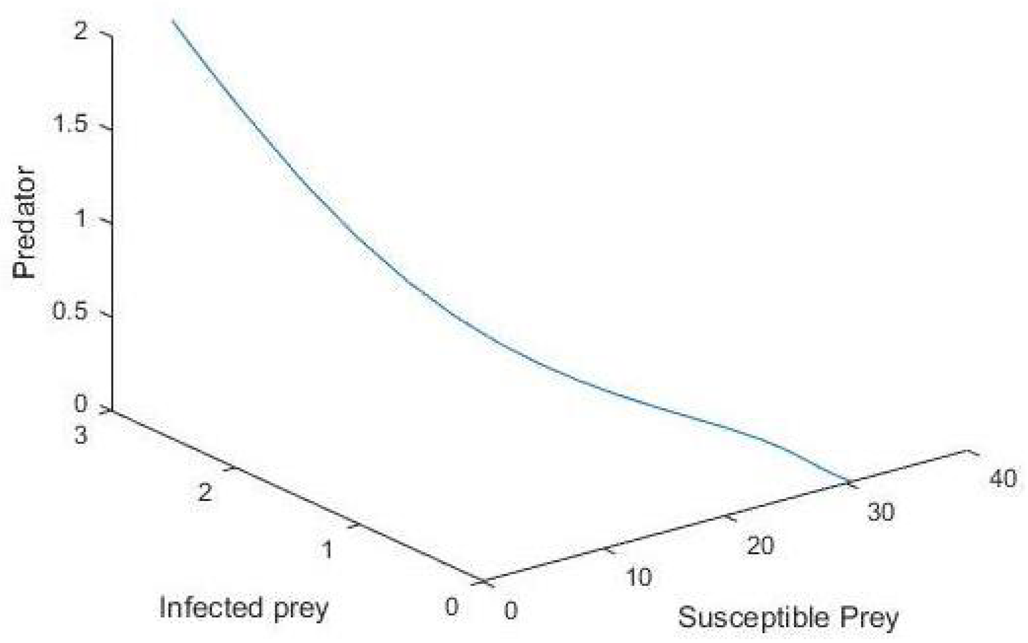
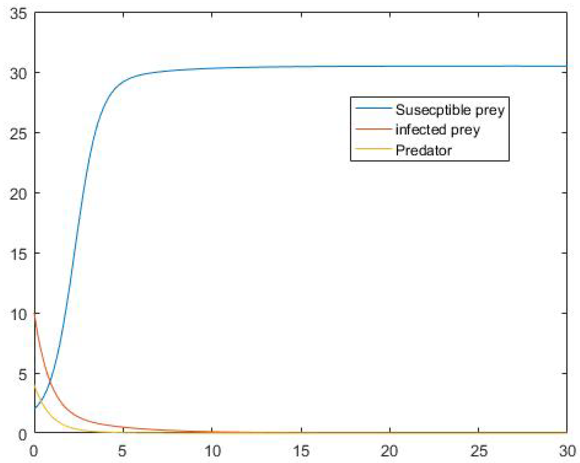
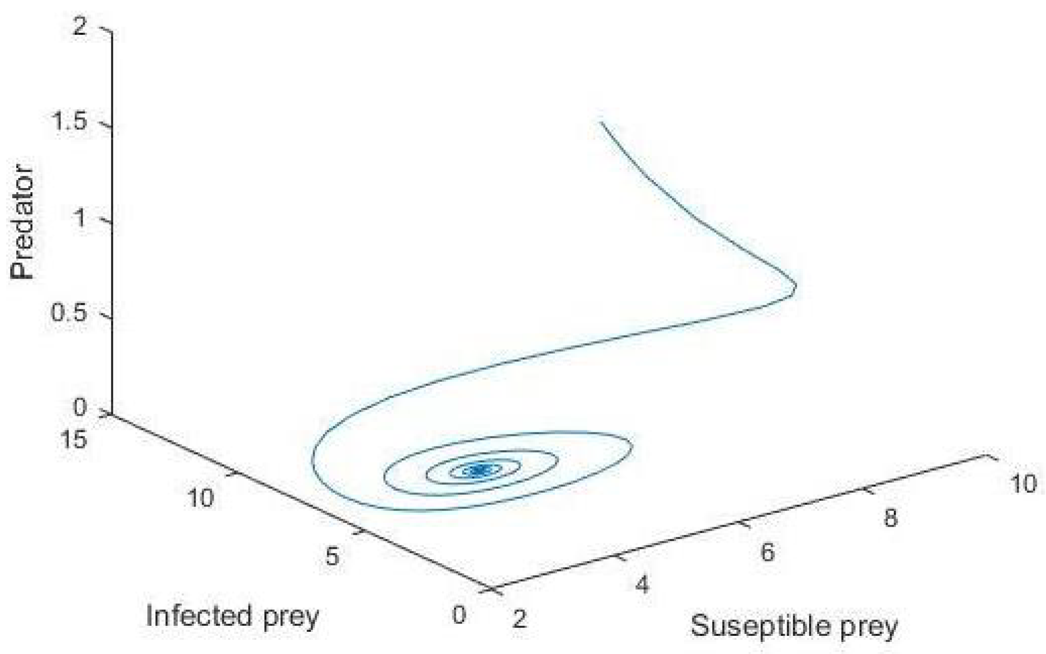
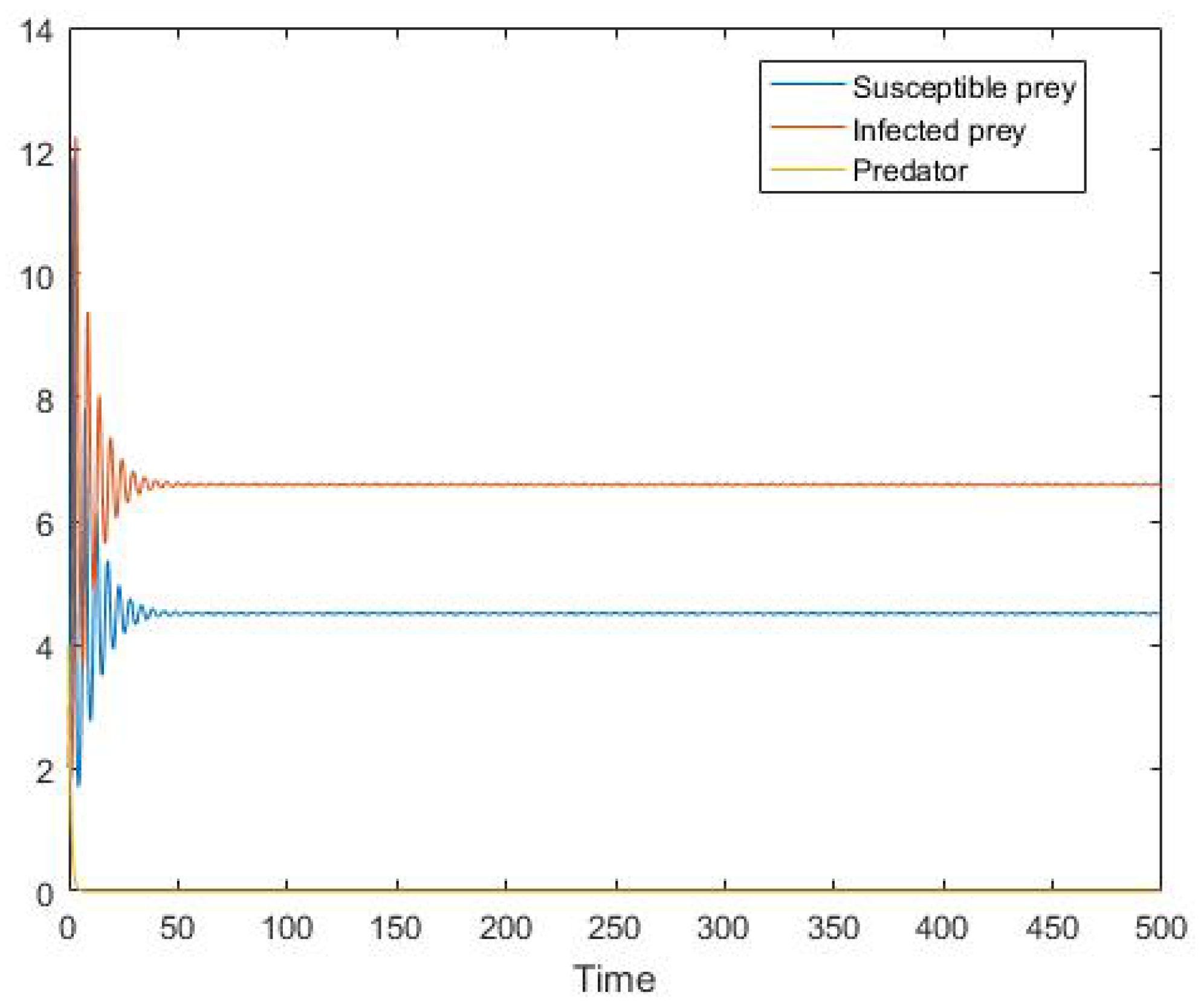
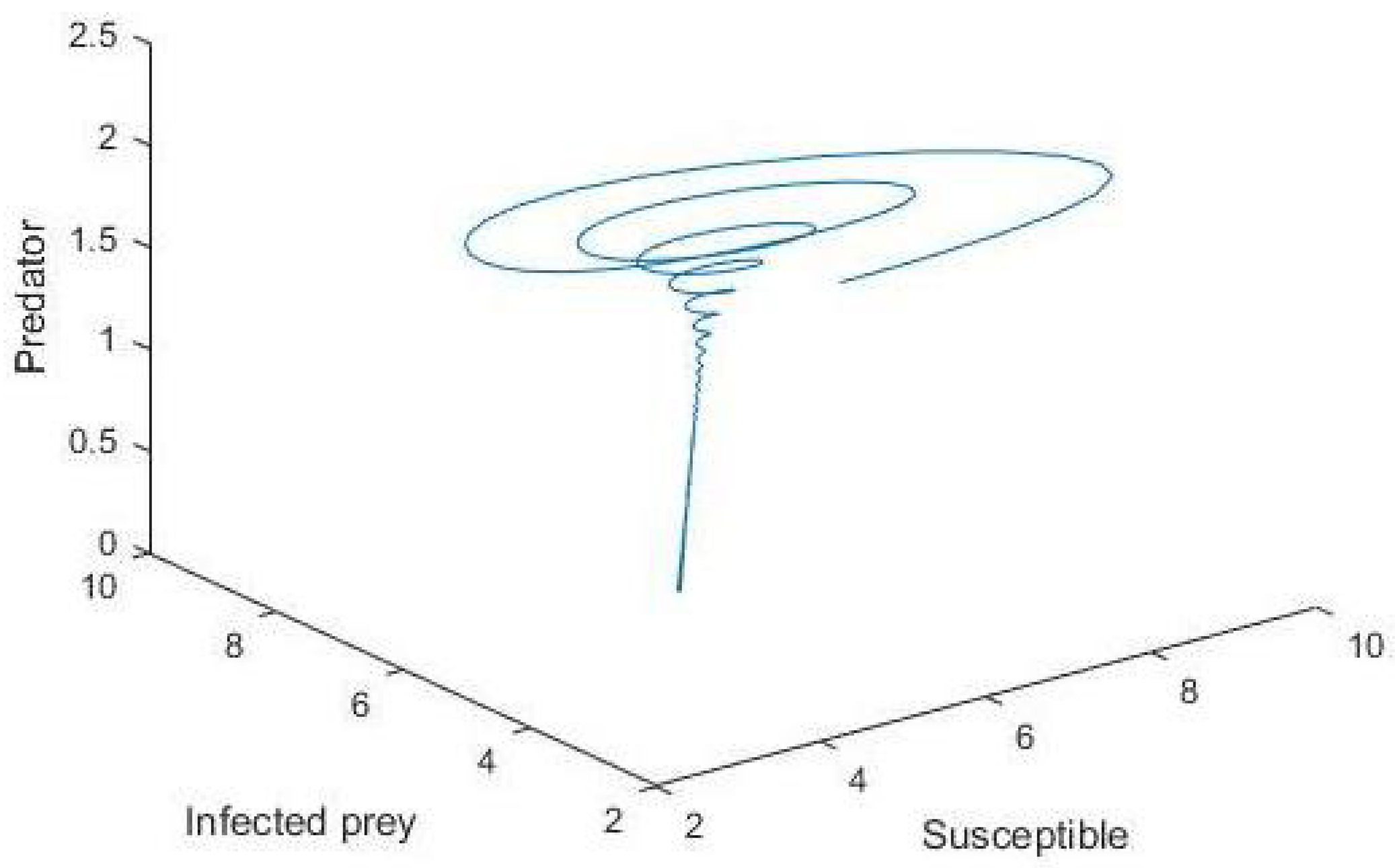
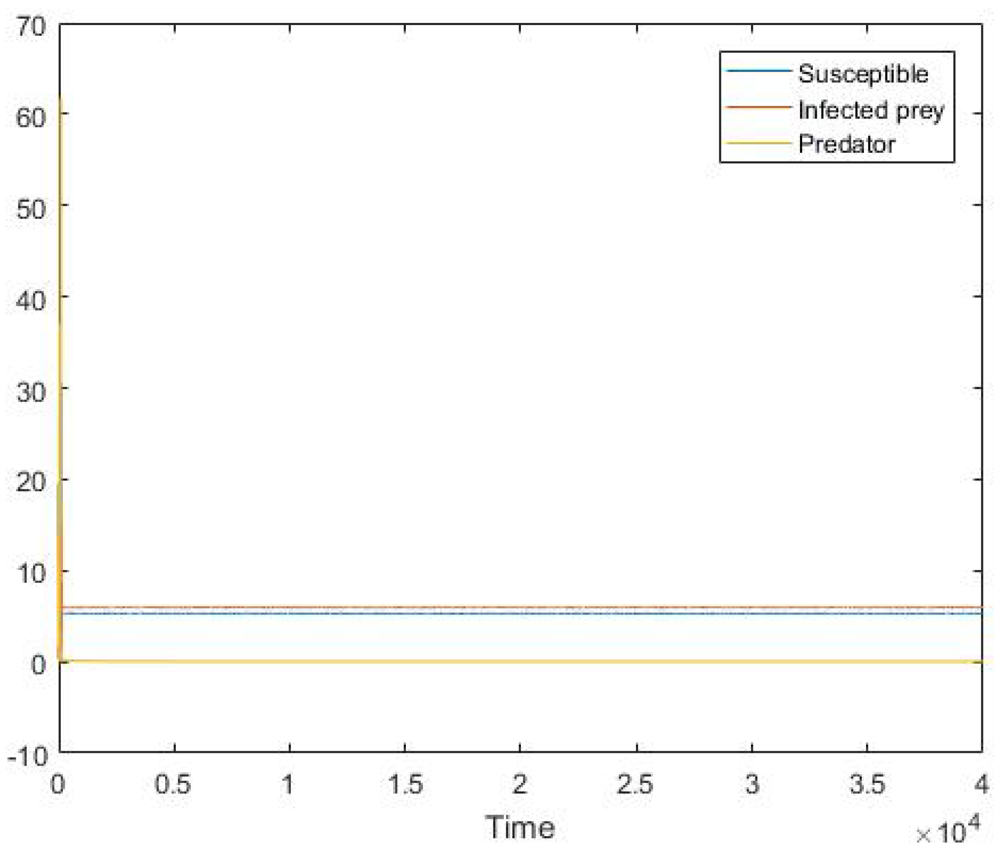
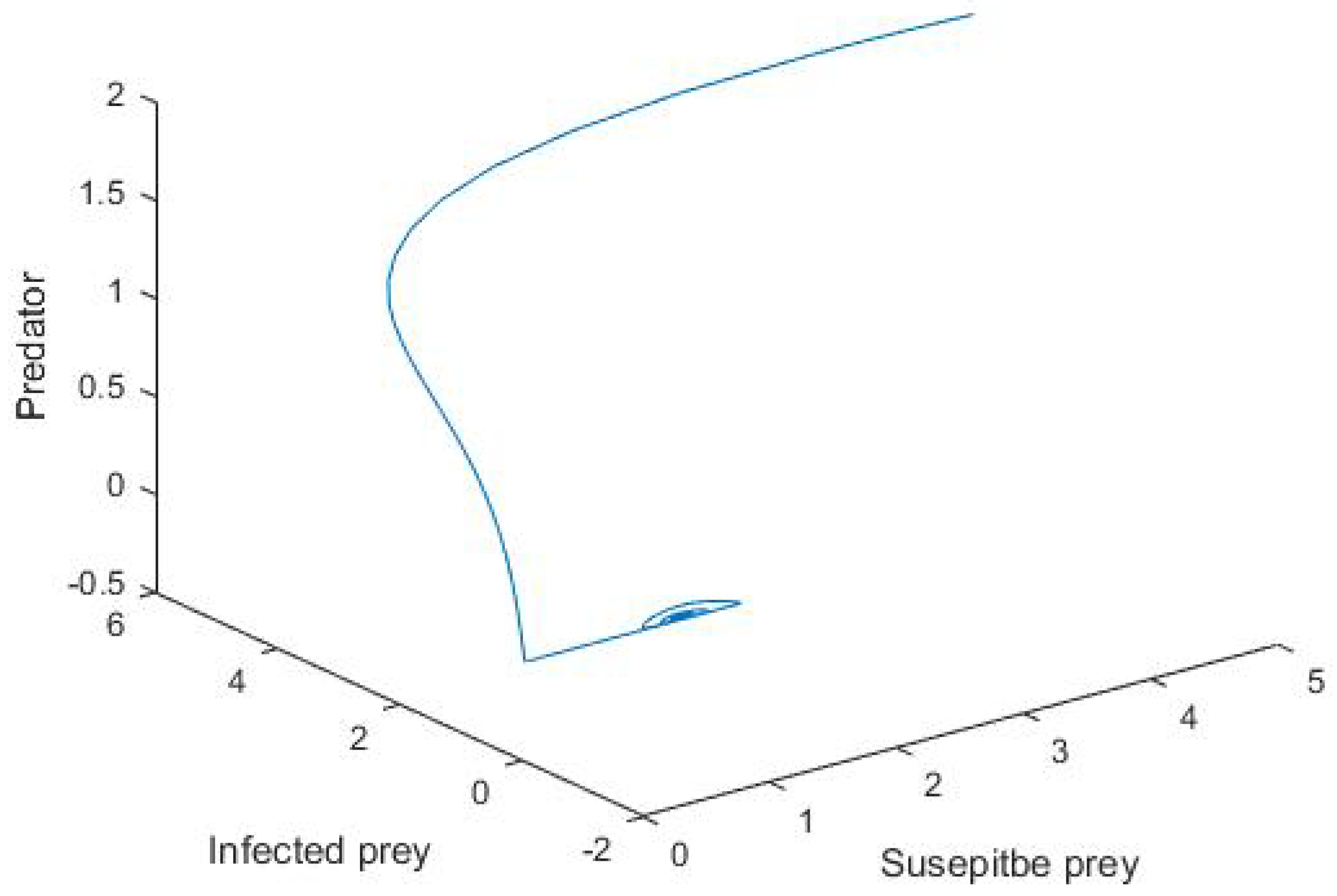
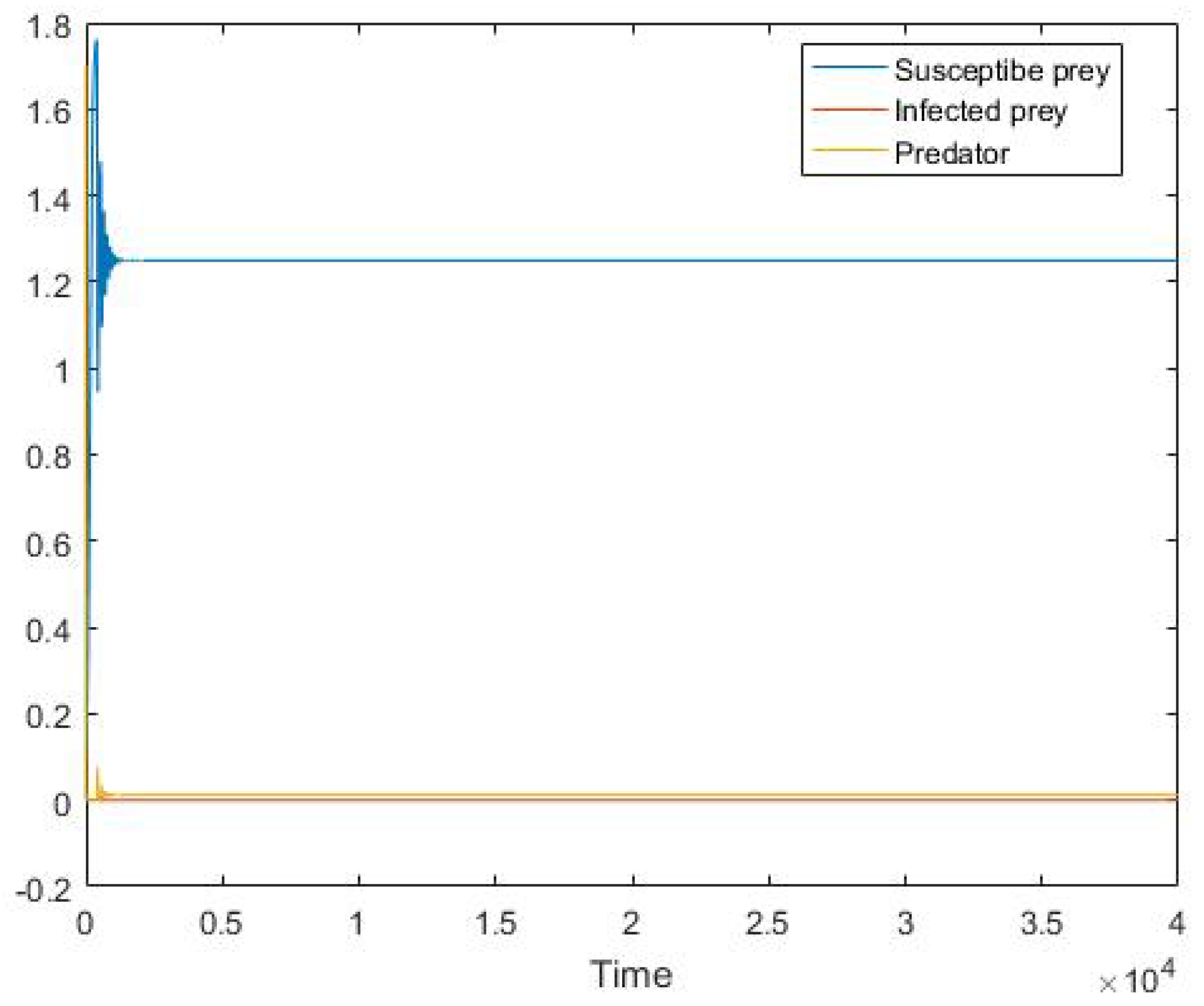
5. Numerical Simulation

In this section, we study the system (1) numerically, starting at different initial points to confirm our obtained analytical results regarding to each equilibrium point. For the following set of hypothetical parameters

$$\begin{array}{cc}\hfill & r=2.1,k=40,m=0.2,\mu =1,b=0.8,c=0.9,g=0.6,\hfill \end{array}$$

(26)

$$\begin{array}{cc}\hfill & h=0.5,E_1=2.2,E_2=0.4,E_3=0.8,\alpha =0.98,\lambda =0.5,\theta =0.5.\hfill \end{array}$$

(27)

System (1) approaches asymptotically to the non-survival point as illustrated in Figure 1 and Figure 2, which is that all of the population will die out because the harvesting rate is greater than the intrinsic growth rate.

If we decrease the value of $E_1$ to $0.5$ and the value of m to $0.02$ then the system approaches the predator free equilibrium point, as shown in Figure 3 and Figure 4.

Note that it is easy to verify that the data in Figure 3 satisfy the conditions (19) and hence Figure 3 confirms the analytical results. Further, for the data

$$\begin{array}{cc}\hfill & r=2.1,k=40,m=0.17,\mu =0.3,b=0.8,c=0.9,g=0.9,\hfill \end{array}$$

(28)

$$\begin{array}{cc}\hfill & h=2.5,E_1=0.5,E_2=0.4,E_3=0.09,\alpha =0.98,\lambda =0.5,\theta =0.5.\hfill \end{array}$$

(29)

that satisfy conditions of Equations (23)–(25), then the system (1) approaches asymptotically to the interior equilibrium point $E_{q4}=(5.2986,5.9304,0.0364)$, as shown in Figure 5 and Figure 6.

For

$$\begin{array}{cc}\hfill & r=0.45,k=40,m=0.5,\mu =1,b=0.8,c=0.9,g=1.6,h=0.9,\hfill \end{array}$$

(30)

$$\begin{array}{cc}\hfill & E_1=0.43,E_2=0.3,E_3=0.5,\alpha =0.9,\lambda =0.5,\theta =0.5,\hfill \end{array}$$

(31)

which satisfies the conditions (20) and (21).

The system approaches asymptotically to the infected free equilibrium point $E_{q3}=(1.25,0,0.0119)$, as shown in Figure 7 and Figure 8.

6. Conclusions

In this article, we explored the interaction of a vulnerable and diseased predator with prey in an eco-epidemiological predator-prey model. In the system, the afflicted predator is liable to harvesting. For all feasible positive equilibrium points, we discovered the key requirements of the parameters of the proposed system for existence as well as asymptotically stable. Harvesting a diseased predator can be considered a biological control to minimize disease transmission and lower the chance of healthy predator extinction. By increasing the rate of harvesting, $E_1$, with respect to the rate of intrinsic growth, then the predator-prey model (1) approaches asymptotically to non-survival point $E_{q1}$ as shown in Figure 1, which is that the entire population will die out.

When we decreased the value of $E_1$ for which $r-E_1$ is positive, we observed that the system (1) approaches the predator free equilibrium point $E_{q2}$ as shown in Figure 3 because $E_{q2}=(\overline{S},\overline{I},0)$ satisfies Equation (6), approaches asymptotically to the infected free equilibrium point $E_{q3}$ as shown in Figure 7, and approaches asymptotically to the interior equilibrium point $E_{q4}$ as shown in Figure 5.

By maximizing an intrinsic biological parameter, we obtain an optimal harvesting strategy that will benefit the population the most. The symmetry properties of the optimal strategy are also discussed. In fact, the mathematical symmetry of the domain is rarely found in the habitat of true populations. However, our arguments show that in general, the rate of harvest should be chosen as minimally as possible. We have obtained that the increasing value of the harvesting with respect to the value of intrinsic growth causes destabilization in the positive equilibrium.

We have solved the model numerically by using MATLAB program (Ode 45 command).

References

1. Nucci, M.C.; Leach, P.G.L. An integrable SIS model. J. Math. Anal. Appl. 2004, 290, 506–518. [Google Scholar] [CrossRef] [Green Version]
2. Nucci, M.C. Jacobi last multiplier and Lie symmetries: A novel application of an old relationship. J. Nonlinear Math. Phys. 2005, 12, 284–304. [Google Scholar] [CrossRef] [Green Version]
3. Nucci, M.C. Using lie symmetries in epidemiology. J. Differ. Equ. 2005, 12, 87–101. [Google Scholar]
4. Leach, P.G.L.; Andriopoulos, K. Application of symmetry and symmetry analyses to systems of first-order equations arising from mathematical modeling in epidemiology. Proc. Inst. Math. Nas Ukr. 2004, 50 Pt 1, 159–169. [Google Scholar]
5. Nucci, M.C.; Leach, P.G.L. Singularity and symmetry analyses of mathematical models of epidemics. S. Afr. J. Sci. 2009, 105, 136–146. [Google Scholar] [CrossRef]
6. Lotka, A.J. Elements of Physical Biology. Nature 1925, 116, 461. [Google Scholar] [CrossRef]
7. Volterra, V. Variations and Fluctuations of the Number of Individuals in Animal Species living together. ICES J. Mar. Sci. 1928, 3, 3–51. [Google Scholar] [CrossRef]
8. Kermack, W.O.; McKendrick, A.G. Contributions to the mathematical theory of epidemics-part I. Proc. R. Soc. Edinb. Sect. A 1927, 115, 700–721. [Google Scholar] [CrossRef] [Green Version]
9. Anderson, R.M.; May, R.M. The invasion, persistence, and spread of infectious diseases within animal and plant communities. Philos. Trans. R. Soc. Biol. Sci. 1986, 314, 533–570. [Google Scholar] [CrossRef]
10. Molla, H.; Sarwardi, S.; Sajid, M. Predator-prey dynamics with Allee effect on predator species subject to intra-specific competition and nonlinear prey refuge. J. Math. Comput. Sci. 2021, 25, 150–165. [Google Scholar] [CrossRef]
11. Mustafa, A.N.; Amin, S.F. A harvested modified Leslie-gower predator-prey model with SIS-disease in predator and prey refuge. J. Duhok-Univ.- Sect. Pure Eng. Sci. 2019, 22, 174–184. [Google Scholar] [CrossRef]
12. Naji, R.K.; Mustafa, A.N. The dynamics of an eco-epidemiological model with nonlinear incidence rate. J. Appl. Math. 2012, 2012, 24. [Google Scholar] [CrossRef]
13. Naji, R.K.; Yaseen, R.M. Modeling and stability analysis of an eco-epidemiological Model. Iraqi J. Sci. 2013, 54, 374–385. [Google Scholar]
14. Greenhalgh, D.; Khan, Q.J.A.; Al-Kharousi, F.A. Eco-epidemiological model with fatal disease in the prey. Nonlinear Anal. Real World Appl. 2020, 53, 103072. [Google Scholar] [CrossRef]
15. Wang, X.; Wang, Z.; Shen, X. Stability and Hopf bifurcation of a fractional-order food chain model with disease and two delays. J. Comput. Nonlinear Dynam. 2020, 15, 034501. [Google Scholar] [CrossRef]
16. Biswas, S.; Saifuddin, M.; Sasmal, S.K.; Samanta, S.; Pal, N.; Ababneh, F.; Chattopadhyay, J. Optimal harvesting and complex dynamics in a delayed eco-epidemiological model with weak Allee effects. Nonlinear Dynam. 2017, 87, 1553–1573. [Google Scholar] [CrossRef]
17. Biswas, S.; Saifuddin, M.; Sasmal, S.K.; Samanta, S.; Pal, N.; Ababneh, F.; Chattopadhyay, J. A delayed prey-predator system with prey subject to the strong Allee effect and disease. Nonlinear Dynam. 2016, 84, 1569–1594. [Google Scholar] [CrossRef]
18. Hu, G.P.; Li, X.L. Stability and Hopf bifurcation for a delayed predator-prey model with disease in the prey. Chaos Solitons Fractals 2012, 45, 229–237. [Google Scholar] [CrossRef]
19. Nandi, S.K.; Mondal, P.K.; Jana, S.; Haldar, P.; Kar, T.K. Prey-predator model with two-stage infection in prey concerning pest control. J. Nonlinear Dynam. 2015, 2015, 948728. [Google Scholar] [CrossRef] [Green Version]
20. Johri, A.; Trivedi, N.; Sisodiya, A.; Sing, B.; Jain, S. Study of a prey-predator model with disease prey. Int. J. Contemp. Math. Sci. 2012, 7, 489–498. [Google Scholar]
21. Sharma, S.; Samanta, G.P. Analysis of a two prey one predator system with disease in the first prey population. Int. J. Dyn. Control 2015, 3, 210–224. [Google Scholar] [CrossRef]
22. Jana, S.; Guria, S.; Das, U.; Kar, T.K.; Ghorai, A. Effect of harvesting and infection on predator in a prey-predator system. Nonlinear Dynam. 2015, 81, 1–14. [Google Scholar] [CrossRef]
23. Shaikh, A.A.; Das, H.; Ali, N. Study of LG-Holling type III predator-prey model with disease in predator. J. Appl. Math. Comput. 2018, 58, 235–255. [Google Scholar] [CrossRef] [Green Version]
24. Xu, R.; Zhang, S.H. Modelling and analysis of a delayed predator-prey model with disease in the predator. Appl. Math. Comput. 2013, 224, 372–386. [Google Scholar] [CrossRef]
25. Zhang, J.S.; Sun, L. Analysis of eco-epidemiological model with epidemic in the predator. J. Biomath. 2005, 20, 157–164. [Google Scholar]
26. Ko, W.; Ryu, K. Qualitative analysis of a predator–prey model with Holling type II functional response incorporating a prey refuge. J. Differ. Equ. 2006, 231, 534–550. [Google Scholar] [CrossRef] [Green Version]
27. Chen, L.; Chen, F.; Chen, L. Qualitative analysis of a predator– prey model with Holling type II functional response incorporating a constant prey refuge. Nonlinear Anal. Real World Appl. 2010, 11, 246–252. [Google Scholar] [CrossRef]
28. Selvam, A.G.M.; Jacob, S.B. Analysis of prey–predator model with holling type II functional response in discrete time. In Proceedings of the International Conference on Current Scenario in Pure and Applied Mathematics (ICCSPAM-2019), Tamil Nadu, India, 3 January 2019; Volume 2, pp. 19–44. [Google Scholar]
29. Jana, S.; Kar, T.K. Modeling and analysis of a prey–predator system with disease in the prey. Chaos Solitons Fractals 2013, 47, 42–53. [Google Scholar] [CrossRef]
30. Prasad, B.S.R.V.; Banerjee, M.; Srinivasu, P.D.N. Dynamics of additional food provided predator-prey system with mutually interfering predators. Math. Biosci. 2013, 246, 176–190. [Google Scholar] [CrossRef]
31. Wang, X.; Zanette, L.; Zou, X. Modelling the fear effect in predator– prey interactions. J. Math. Biol. 2016, 73, 1179–1204. [Google Scholar] [CrossRef] [PubMed]
32. Lee, H.A.A.E.S.; Jang, B. Dynamic analysis of fractional-order predator–prey biological economic system with Holling type II functional response. Nonlinear Dyn. 2019, 96, 407–416. [Google Scholar] [CrossRef]
33. Shaikh, A.A.; Das, H.; Sarwardi, S. Dynamics of an eco-epidemiological system with disease in competitive prey species. J. Appl. Math. Comput. 2020, 62, 525–545. [Google Scholar] [CrossRef]
34. Bera, S.P.; Maiti, A.; Samanta, G.P. Dynamics of a food chain model with herd behaviour of the prey. Model. Earth Syst. Environ. 2016, 2, 1–9. [Google Scholar] [CrossRef] [Green Version]
35. Das, S.; Mahato, P.; Mahato, S.K. Disease control prey–predator model incorporating prey refuge under fuzzy uncertainty. Model. Earth Syst. Environ. 2021, 7, 2149–2166. [Google Scholar] [CrossRef]
36. Das, K.P. A study of harvesting in a predator-prey model with disease in both populations. Math. Methods Appl. Sci. 2016, 39, 2853–2870. [Google Scholar] [CrossRef]
37. Kant, S.; Kumar, V. Stability analysis of predator-prey system with migrating prey and disease infection in both specise. Appl. Math. Model. 2017, 42, 509–539. [Google Scholar] [CrossRef]
38. Dai, G.; Tang, M. Coexistence region and global dynamics of a harvested predator-prey system. SIAM J. Appl. Math. 1998, 58, 193–210. [Google Scholar] [CrossRef]
39. Guin, L.N.; Acharya, S. Dynamic behaviour of a reaction-diffusion predator-prey model with both refuge and harvesting. Nonlinear Dynam. 2017, 88, 1501–1533. [Google Scholar] [CrossRef]
40. Clark, C.W. Mathematical Bioeconomics: The Optimal Management of Renewable Resources, 2nd ed.; Wiley: New York, NY, USA, 1990. [Google Scholar]
41. Bairagi, N.; Chaudhuri, S.; Chattopadhyay, J. Harvesting as a disease control measure in an ecoepidemiological system—A theoretical study. Math. Biosci. 2009, 217, 134–144. [Google Scholar] [CrossRef] [PubMed]
42. Hethcote, H.W.; Wang, W.; Han, L.; Ma, Z. A predator-prey model with infected prey. Theor. Popul. Biol. 2014, 34, 849–858. [Google Scholar] [CrossRef]
43. Azar, C.; Holmberg, J.; Lindgren, K. Stability analysis of harvesting in a predator–prey model. J. Theor. Biol. 1995, 174, 13–19. [Google Scholar] [CrossRef]
44. Ge, Z.; Yan, J. Hopf bifurcation of a predator-prey system with stage structure and harvesting. Nonlinear Anal. Theory Methods Appl. 2011, 74, 652–660. [Google Scholar] [CrossRef]
45. Brauer, F.; Sanchez, D. Constant rate population harvesting: Equilibrium and stability. Theor. Popul. Biol. 1975, 8, 12–30. [Google Scholar] [CrossRef]
46. Brauer, F.; Soudack, A.C. Stability regions and transition phenomena for harvested predator–prey systems. J. Math. Biol. 1979, 7, 319–337. [Google Scholar] [CrossRef]
47. Xiao, D.; Ruan, S. Bogdanov–Takens bifurcations in predator–prey systems with constant rate harvesting. Fields Inst. Commun. 1999, 21, 493–506. [Google Scholar]
48. Beddington, J.R.; Cooke, J.G. Harvesting from a prey–predator complex. Ecol. Model. 1982, 14, 155–177. [Google Scholar] [CrossRef]
Figure 1. System (1) approaches asymptotically stable point E q 1 under the parameter values in (26) and (27).
Symmetry 13 02179 g001
Figure 2. The time series starts at ( 2 , 3 , 4 ) and the solution approaches asymptotically to the disease and predator-free equilibrium point ( 30.4648 , 0 , 0 ) .
Symmetry 13 02179 g002
Figure 3. System (1) approaches the asymptotically stable point E q 2 = ( 4.4896 , 6.5828 , 0 ) under the parameter values (26) and (27) where E 1 = 0.5 and m = 0.02 .
Symmetry 13 02179 g003
Figure 4. The time series starts at ( 2 , 3 , 4 ) and the solution approaches asymptotically the point E q 2 = ( 4.4896 , 6.5828 , 0 ) .
Symmetry 13 02179 g004
Figure 5. System (1) approaches the asymptotically stable point E q 4 under the parameter values in (28) and (29).
Symmetry 13 02179 g005
Figure 6. The time series starts at ( 1.1 , 1 , 1.7 ) , and the solution approaches the epidemic positive point ( 5.2986 , 5.9304 , 0.0364 ) .
Symmetry 13 02179 g006
Figure 7. System (1) approaches asymptotically the stable point E q 3 under the parameter values in (30) and (31).
Symmetry 13 02179 g007
Figure 8. The time series starts at ( 1.1 , 1 , 1.7 ) , and the solution approaches the infected free equilibrium point E q 3 = ( 1.25 , 0 , 0.0119 ) .
Symmetry 13 02179 g008