On a Conjecture for the One-Dimensional Perturbed Gelfand Problem for the Combustion Theory

Abstract

We investigate the well-known one-dimensional perturbed Gelfand boundary value problem and approximate the values of ${\alpha }_0,{\lambda }_{*}$ and ${\lambda }^{*}$ such that this problem has a unique solution when $0<\alpha <{\alpha }_0$ and $\lambda >0,$ and has three solutions when $\alpha >{\alpha }_0$ and ${\lambda }_{*}<\lambda <{\lambda }^{*}.$ The solutions of this problem are always even functions due to its symmetric boundary values and autonomous characteristics. We use numerical computation to show that $4.0686722336<{\alpha }_0<4.0686722344$. This result improves the existing result for ${\alpha }_0\approx 4.069$ and increases the accuracy of ${\alpha }_0$ to ${10}^{-8}.$ We developed an algorithm that reduces errors and increases efficiency in our computation. The interval of $\lambda$ for this problem to have three solutions for given values of $\alpha$ is also computed with accuracy up to ${10}^{-14}.$

1. Introduction

We study the well-known one-dimensional perturbed Gelfand two-point boundary value problem (BVP) [1,2]

$$\left\{\begin{array}{c}{u}^{\prime \prime }\left(t\right)+\lambda exp\left(\frac{\alpha u}{\alpha +u}\right)=0,-1<t<1\\ u(-1)=u\left(1\right)=0\end{array}\right.\left(1\right)$$

(1)

where $\lambda >0$ is the Frank-Kamenetskii parameter, or ignition parameter, $\alpha >0$ is the activation energy parameter, $u\left(t\right)$ is the dimensionless temperature, and the reaction term $exp\left(\frac{au}{a+u}\right)$ is the temperature dependence obeying the simple arrhenius reaction-rate law in irreversible chemical reaction kinetics. It has been a long-standing conjecture [3,4,5,6,7,8,9,10,11,12,13,14,15,16] about the shapes of evolutionary bifurcation curves and the exact multiplicity of positive solutions of (1) with $\alpha >0.$ In particular, Hastings and McLeod [3] proved the bifurcation curve is S-shaped on the $(\lambda ,$${\left|\right|u\left|\right|}_{\infty })$plane when $\alpha$ is large enough. Therefore, for each $\lambda >0$, there exist at least two positive solutions when $\alpha$ is sufficiently large. Brown et al. [4] obtained a better result by finding an estimation of $\alpha >4.25.$ Wang [5] proved that BVP (1) has multiple solutions when $\alpha >4.4967.$ This upper bound was improved to 4.35 by Korman and Li [6]. The most recent result about this problem is from S. Y. Huang and S. H. Wang [8,9], proving that BVP (1) has three solutions when $\alpha >$$4.069$. We prove that this problem has a unique solution for $\alpha <4.0686722336$ and has three solutions when $\alpha >4.0686722344$. The interval of $\lambda$ for BVP (1) to have three solutions for given $\alpha$ value is also computed with accuracy up to ${10}^{-14}.$

It is well-known that the solutions of this problem are always even functions due to its symmetric boundary values and autonomous characteristics. Since the equation in (1) is a quasi-linear differential equation, we will find an implicit general solution of this problem first and apply the boundary values to it. Because $u^{\prime \prime }\left(t\right)<0$ is always true and $u(-1)=u\left(1\right)=0$, $u\left(t\right)$ has only one stagnation point that must be a maximum. For developing our algorithm, we first use this property and basic calculus techniques to convert BVP (1.1) to an integral equation.

Assuming that $t_0$ is the stagnation point for $-1<t_0<1$, we consider the following initial value problem

$$\left\{\begin{array}{c}{u}^{\prime \prime }\left(t\right)+\lambda exp\left(\frac{\alpha u\left(t\right)}{\alpha +u\left(t\right)}\right)=0,\\ u\left(t_0\right)=C,u^{\prime }\left(t_0\right)=0.\end{array}\right.\left(2\right)$$

(2)

Integrating the equation in (2) once, we get the following integral equation

$$u^{\prime 2}\left(t\right)+2\lambda {\int }_{t_0}^{t}exp\left(\frac{\alpha u\left(s\right)}{\alpha +u\left(s\right)}\right)u^{\prime }\left(s\right)ds=0\left(3\right)$$

(3)

or

$$u^{\prime 2}\left(t\right)=-2\lambda {\int }_C^{u\left(t\right)}exp\left(\frac{\alpha v}{\alpha +v}\right)dv>0.\left(4\right)$$

(4)

Since $u\left(t_0\right)=C$ is the maximum, one has that $u^{\prime }\left(t\right)\ge 0$ for $-1<t<t_0$ and $u^{\prime }\left(t\right)\le 0$ for $t_0<t<1.$ Hence we can write (4) as follows:

$$u^{\prime }\left(t\right)=\left\{\begin{array}{c}\sqrt{2\lambda }\sqrt{{\int }_{u\left(t\right)}^{C}exp\left(\frac{\alpha v}{\alpha +v}\right)dv},-1<t<t_0,\\ -\sqrt{2\lambda }\sqrt{{\int }_{u\left(t\right)}^{C}exp\left(\frac{\alpha v}{\alpha +v}\right)dv},t_0<t<1.\end{array}\right.\left(5\right)$$

(5)

Integrating (5) again, we get the implicit solution of (2) as follows:

$${\int }_{t_0}^t{\left({\int }_{u\left(t\right)}^{C}exp\left(\frac{\alpha v}{\alpha +v}\right)dv\right)}^{-1/2}{u}^{\prime }\left(t\right)dt=\left\{\begin{array}{c}\sqrt{2\lambda }(t-t_0),-1<t<t_0\\ -\sqrt{2\lambda }(t-t_0),t_0<t<1\end{array}\right.\left(6\right)$$

(6)

or

$${\int }_C^{u\left(t\right)}{\left({\int }_w^{C}exp\left(\frac{\alpha v}{\alpha +v}\right)dv\right)}^{-1/2}dw=\left\{\begin{array}{c}\sqrt{2\lambda }(t-t_0),-1<t<t_0\\ -\sqrt{2\lambda }(t-t_0),t_0<t<1\end{array}.\right.\left(7\right)$$

(7)

Applying the boundary conditions of (1) to (7), we get

$$\begin{array}{c}{\int }_C^0{\left({\int }_w^{C}exp\left(\frac{\alpha v}{\alpha +v}\right)dv\right)}^{-1/2}dw=\sqrt{2\lambda }(-1-t_0),\end{array}\left(8\right)$$

(8)

and

$$\begin{array}{c}{\int }_C^0{\left({\int }_w^{C}exp\left(\frac{\alpha v}{\alpha +v}\right)dv\right)}^{-1/2}dw=-\sqrt{2\lambda }(1-t_0).\end{array}\left(9\right)$$

(9)

It follows (8) and (9) that $t_0=0$ and

$$\begin{array}{c}{\int }_C^{u\left(t\right)}{\left({\int }_w^{C}exp\left(\frac{\alpha v}{\alpha +v}\right)dv\right)}^{-1/2}dw=\left\{\begin{array}{c}\sqrt{2\lambda }t,-1<t<0,\\ -\sqrt{2\lambda }t,0<t<1.\end{array}\right.\end{array}\left(10\right)$$

(10)

Hence, we have

$$\begin{array}{c}{\int }_0^C{\left({\int }_w^{C}exp\left(\frac{\alpha v}{\alpha +v}\right)dv\right)}^{-1/2}dw=\sqrt{2\lambda }.\end{array}\left(11\right)$$

(11)

Equation (11) has a unique solution C for certain values of $\alpha$ and $\lambda$ if and only if BVP (1) has a unique solution $u\left(t\right)$ for the same values of $\alpha$ and $\lambda$. Furthermore, the number of solutions C to Equation (11) is corresponding to the number of solutions of BVP (1) for the given values of $\alpha$ and $\lambda$. In the following sections, we investigate the values of ${\alpha }_0$, ${\lambda }_{*}$ and ${\lambda }^{*}$ such that (11) has a unique solution when $0<\alpha <{\alpha }_0$ and $\lambda >0,$ and has three solutions when $\alpha >{\alpha }_0$ and ${\lambda }_{*}<\lambda <{\lambda }^{*}.$ In Section 2, we prove that BVP (1) has three solutions when $\alpha \ge 4.06867225$ for some values of $\lambda$ and provide the graphical solutions for some values of $\alpha$ and $\lambda$. In Section 3, we prove that there is a positive number $ϵ$ such that BVP (1) has a unique solution for all values of $\lambda >0$ and $\alpha \in (0,4+ϵ).$ Based on the results in Section 2 and Section 3, an ${\alpha }_0$ must exist. We prove that ${\alpha }_0$ is between $4.0686722336$ and $4.0686722344$ in Section 4. In Section 5, we calculate and draw a graph that displays a region of $\alpha$ and $\lambda$ in which BVP (1) has three solutions. This region shows a clear relationship between $\alpha$, ${\lambda }_{*}$ and ${\lambda }^{*}.$ We also draw the two corresponding solutions when $\sqrt{\frac{\lambda }{2}}$ is exactly the maximum or minimum of $H(x,\alpha ).$ The article is concluded at Section 6.

2. Three Solutions of BVP (1), Their Graphical Representations and the Corresponding $\mathbf{\lambda }$ Interval when $\mathbf{\alpha }\ge \mathbf{4}.\mathbf{06867225}$

As we have explained in the previous section, we will work with Equation (11). All the calculations in this article use 32 bit precision.

Since numerical computation of double integrals is time-consuming and also causes large errors, we first convert the left-side of (11) into a single integral. In fact, this is a crucial move for this computation to be possible. Using power series expansion, we have

$$\begin{array}{c}{\int }_w^{C}exp\left(\frac{\alpha v}{\alpha +v}\right)dv=e^a{\int }_w^{C}exp\left(-\frac{{\alpha }^2}{\alpha +v}\right)dv\hfill \\ =e^a{\int }_w^C\sum _{n=0}^{\infty }\frac{{(-1)}^n{\alpha }^{2n}}{n!{(a+v)}^n}dv=e^{\alpha }g(w,C,\alpha ),\hfill \end{array}\left(12\right)$$

(12)

where

$$\begin{array}{c}g(w,x,\alpha )=x-w-{\alpha }^{2}ln\left(\frac{a+x}{a+w}\right)+\sum _{n=2}^{\infty }\frac{{(-1)}^{n-1}{\alpha }^{2n}}{(n-1)n!}\left(\frac{1}{{(a+x)}^{n-1}}-\frac{1}{{(a+w)}^{n-1}}\right)\end{array}\left(13\right)$$

(13)

and

$$\begin{array}{c}\frac{d}{dx}g(w,x,\alpha )=exp\left(-\frac{{\alpha }^2}{\alpha +x}\right)=exp\left(-\alpha \right)exp\left(\frac{\alpha x}{\alpha +x}\right),\\ \frac{d}{dw}g(w,x,\alpha )=-exp\left(-\frac{{\alpha }^2}{\alpha +w}\right)=-exp\left(-\alpha \right)exp\left(\frac{\alpha w}{\alpha +w}\right).\end{array}\left(14\right)$$

(14)

Putting (12) into (11), we have

$$\begin{array}{c}{e}^{-\frac{\alpha }{2}}{\int }_0^C\frac{dw}{\sqrt{g(w,C,\alpha )}}=\sqrt{2\lambda }.\end{array}\left(15\right)$$

(15)

When w approaches C, the denominator of the integrand in (15) approaches 0, which causes very large error of the computation. To overcome this problem, we use (12) and integrate by parts to get

$$\begin{array}{c}{\int }_0^C\frac{1}{\sqrt{g(w,C,\alpha )}}dw=-2e^a{\int }_0^{C}exp\left(-\frac{\alpha w}{\alpha +w}\right)d\sqrt{g(w,C,\alpha )}\hfill \\ =2e^a\sqrt{g(0,C,\alpha )}-2{\alpha }^2{e}^a{\int }_0^C\frac{exp\left(-\frac{\alpha w}{\alpha +w}\right)}{{(\alpha +w)}^2}\sqrt{g(w,C,\alpha )}dw.\hfill \end{array}\left(16\right)$$

(16)

Putting (16) into (15), we have

$$\begin{array}{c}H(C,\alpha )=\sqrt{\frac{\lambda }{2}},\hfill \end{array}\left(17\right)$$

(17)

where

$$\begin{array}{c}H(x,\alpha )=e^{\frac{\alpha }{2}}\sqrt{g(0,x,\alpha )}-{\alpha }^2{e}^{-\frac{\alpha }{2}}{\int }_0^x\frac{e^{\frac{{\alpha }^2}{\alpha +w}}\sqrt{g(w,x,\alpha )}}{{(\alpha +w)}^2}dw.\hfill \end{array}\left(18\right)$$

(18)

It follows (11) that $H(x,\alpha )>0$ for $x>0,$$\underset{x\to 0}{lim}H(x,\alpha )=0$ and $\underset{x\to \infty }{lim}H(x,\alpha )=\infty .$ Therefore, Equation (17) has at least one solution for any $\lambda >0$, and whether Equation (17) has multiple positive roots depends on the number of extreme values of $H(x,\alpha )$ and the value of $\lambda .$ If $H(x,\alpha )$ has one maximum and one minimum, and $\sqrt{\frac{\lambda }{2}}$ is between them, (17) must have three roots. If $\sqrt{\frac{\lambda }{2}}$ is exactly the maximum or minimum of $H(x,\alpha ),$ (17) has exactly two roots (the horizontal line at value $\sqrt{\frac{\lambda }{2}}$ meets the curve of $H(x,\alpha )$ at this maximum point and also cuts the curve at a point to the right of the maximum point, or meets the curve of $H(x,\alpha )$ at this minimum point and cuts the curve at a point to the left of the minimum point). Otherwise there is only one root.

Due to the fact that $H(x,\alpha )$ is a function with an integral, it is difficult to find the extremum by analysis. We now use numerical method to find the extrema, or stagnation points of $H(x,\alpha ).$ Let

$$\begin{array}{c}{H}^{\prime }(x,\alpha )=0,\hfill \end{array}\left(19\right)$$

(19)

where

$$\begin{array}{c}{H}^{\prime }(x,\alpha )=\frac{1}{2\sqrt{g(0,x,\alpha )}}{e}^{\frac{\alpha x}{\alpha +x}-\frac{\alpha }{2}}-\frac{{\alpha }^2{e}^{\frac{\alpha x}{\alpha +x}-\frac{3\alpha }{2}}}{2}{\int }_0^x\frac{e^{\frac{{\alpha }^2}{\alpha +w}}}{{(\alpha +w)}^2\sqrt{g(w,x,\alpha )}}dw\hfill \\ =\frac{e^{\frac{\alpha x}{\alpha +x}-\frac{\alpha }{2}}}{2\sqrt{g(0,x,\alpha )}}-e^{\frac{\alpha x}{\alpha +x}+\frac{\alpha }{2}}\sqrt{g(0,x,\alpha )}\hfill \\ +2{\alpha }^2{e}^{\frac{\alpha x}{\alpha +x}-\frac{3\alpha }{2}}{\int }_0^x\frac{({\alpha }^2+\alpha +w)exp\left(\frac{2{\alpha }^2}{\alpha +w}\right)\sqrt{g(w,x,\alpha )}}{{(\alpha +w)}^4}dw.\hfill \end{array}\left(20\right)$$

(20)

Taking out the common factor, we consider the following equivalent equation of (19):

$$\begin{array}{c}{H}_1(x,\alpha )=0\hfill \end{array}\left(21\right)$$

(21)

where

$$\begin{array}{c}{H}_1(x,\alpha )=\frac{1}{2}{e}^{-\alpha }-\frac{{\alpha }^2{e}^{-2\alpha }}{2}\sqrt{g(0,x,\alpha )}{\int }_0^x\frac{e^{\frac{{\alpha }^2}{\alpha +w}}}{{(\alpha +w)}^2\sqrt{g(w,x,\alpha )}}dw\hfill \\ =\frac{e^{-\alpha }}{2}+2{\alpha }^2{e}^{-2\alpha }\sqrt{g(0,x,\alpha )}{\int }_0^x\frac{({\alpha }^2+\alpha +w)e^{\frac{2{\alpha }^2}{\alpha +w}}\sqrt{g(w,x,\alpha )}}{{(\alpha +w)}^4}dw-g(0,x,\alpha ).\hfill \end{array}\left(22\right)$$

(22)

We will find the roots of (21) by Newton’s method with the following iteration formula:

$$\begin{array}{c}{C}_{n+1}=C_n-\frac{H_1(C_n,\alpha )}{H_1^{\prime }(C_n,\alpha )},\hfill \end{array}\left(23\right)$$

(23)

where

$$\begin{array}{c}{H}_1^{\prime }(x,\alpha )=\left(\frac{{\alpha }^2{e}^{-2\alpha }}{\sqrt{g(0,x,\alpha )}}{\int }_0^x\frac{({\alpha }^2+\alpha +w)e^{\frac{2{\alpha }^2}{\alpha +w}}}{{(\alpha +w)}^4}\left(\sqrt{g(w,x,\alpha )}+\frac{g(0,x,\alpha )}{\sqrt{g(w,x,\alpha )}}\right)dw-1\right)e^{-\frac{{\alpha }^2}{\alpha +x}}.\hfill \end{array}\left(24\right)$$

(24)

We implemented our algorithm using Mathematica to compute the x values where the extremum values occur and the corresponding extremum values of $H(x,\alpha )$ for several values of $\alpha$ nearby and greater than 4, and results are recorded in the following table.

Table 1. Extrema distribution of $H(x,\alpha )$.

$\mathit{\alpha }$	Maximum Point, Maximum Value	Minimum Point, Minimum Value
$\alpha =5$	2.35412603926,0.7622268370643	15.4140975304,0.6623753601164
$\alpha =\frac{41}{10}$	4.12779060841,0.8056758270208	5.89882206503,0.8049337881022
$\alpha =\frac{407}{100}$	4.72119906322,0.8083766697684	5.08174477492,0.8083701558394
$\alpha =\frac{4069}{1000}$	4.80822906947,0.8084759211837	4.98729736470,0.8084751221088
$\alpha =\frac{40687}{10000}$	4.87059453904,0.8085061618507	4.92270715483,0.8085061421477
$\alpha =\frac{4068675}{1000000}$	4.88833456795,0.8085087047901	4.90478174091,0.8085087041707
$\alpha =\frac{40686725}{10000000}$	4.89399971797,0.8085089597373	4.89909805248,0.8085089597189
$\alpha =\frac{406867225}{100000000}$	4.8959271892,0.80850895253056	4.89716872734,0.8085089852527

shows that when $\alpha$ gets closer and closer to 4, the two extremum points of $H(x,\alpha )$ get closer and closer, with the extremum points converging to a value between $4.8959271892$ and $4.8971687273,$ and the extremum values converging to a value between $0.8085089852527$ and $0.80850895253056.$

When $\alpha \ge \frac{406867225}{100000000}$ and the value of $\sqrt{\frac{\lambda }{2}}$ is between $H_{min}\left(\alpha \right)$and $H_{max}\left(\alpha \right),$ where $H_{min}\left(\alpha \right)$and $H_{max}\left(\alpha \right)$ are the minimum value and the maximum value of $H(x,\alpha )$, respectively, Equation (17) has three roots, which are separated by the extreme points. When $\alpha$ changes from $4.07$ to $4.06867225$ and$\sqrt{\frac{\lambda }{2}}\in (H_{min},H_{max})$ or $\lambda \in (2H_{min}^2\left(\alpha \right),2H_{max}^2\left(\alpha \right)),$$2H_{max}^2\left(\alpha \right)-2H_{min}^2\left(\alpha \right)$ is very small and the allowable error decreases from ${10}^{-6}$ to ${10}^{-13},$ which means that $\delta$ decreases from ${10}^{-6}$ to ${10}^{-13}$as $\alpha$ decreases from $4.07$ to $4.06867225$ when we set $2H_{max}^2\left(\alpha \right)-2H_{min}^2\left(\alpha \right)<\delta$ in our numerical calculation. This is almost impossible if $\lambda$ is chosen randomly, but we can manage to work it out by selecting $\lambda =\frac{{\left(H_{max}\left(\alpha \right)+H_{min}\left(\alpha \right)\right)}^2}{2}.$

When $\alpha \ge \frac{406867225}{100000000},$ we use Newton’s method and the Mathematica language to find the roots of (17) by choosing $\lambda =\frac{{\left(H_{max}\left(\alpha \right)+H_{min}\left(\alpha \right)\right)}^2}{2},$ i.e., $\sqrt{\frac{\lambda }{2}}=\frac{H_{max}\left(\alpha \right)+H_{min}\left(\alpha \right)}{2}$. The iteration formula here is as follows:

$$\begin{array}{c}{C}_{n+1}=C_n-\frac{H(C_n,\alpha )-\sqrt{\lambda /2}}{H^{\prime }(C_n,\alpha )},\hfill \end{array}\left(25\right)$$

(25)

where $H(x,\alpha )$ and $H^{\prime }(x,\alpha )$ are calculated with (18) and (20), respectively. For several values of $\alpha$ that are near and greater than 4, we performed some computation. The range of each $\lambda$ in this table is the value of $\lambda$ for which Equation (17) has three roots with the corresponding value of $\alpha .$ The three roots in the table are the roots of Equation (17) corresponding to the given values of $\alpha$ and $\sqrt{\frac{\lambda }{2}}.$ Our results are recorded in the following table.

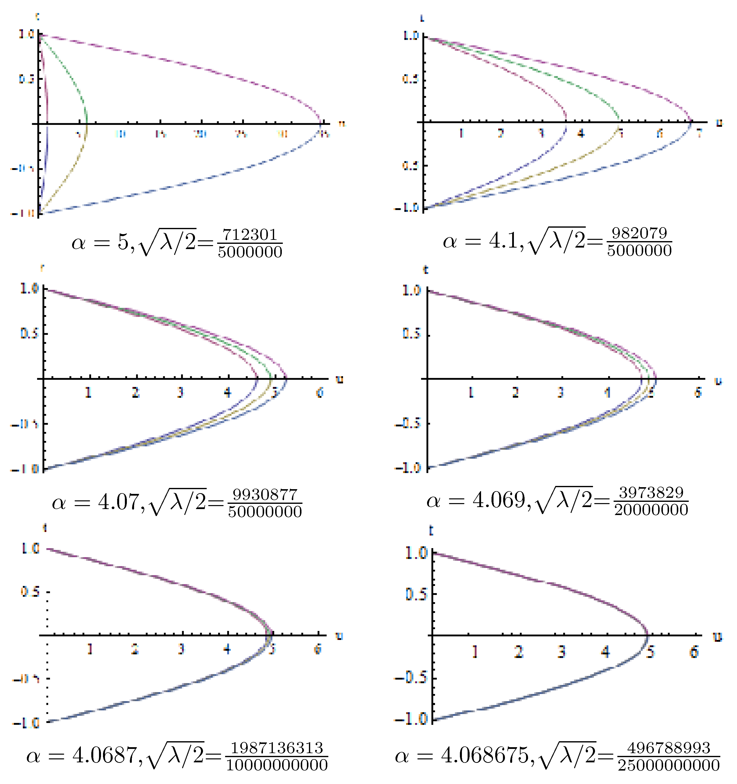
Remark 1.

When $\alpha =4.06876225,$ 

Table 2. The range of $\lambda$ and three roots of (17).

$\mathit{\alpha }$	$\sqrt{\mathit{\lambda }/2}$	The Range of $\mathit{\lambda }$	Root 1, 2, 3
$\alpha =5$	$\frac{356150549}{500000000}$	$\begin{array}{c}(0.87748223507259,\hfill \\ 1.16197948072369)\hfill \end{array}$	$\begin{array}{c}1.09189215963\hfill \\ 5.87905880437\hfill \\ 34.52806380173\hfill \end{array}$
$\alpha =4.1$	$\frac{805304807}{1000000000}$	$\begin{array}{c}(1.29583680370177,\hfill \\ 1.29822705386534)\hfill \end{array}$	$\begin{array}{c}3.62057846489\hfill \\ 4.93384850317\hfill \\ 6.728088610684\hfill \end{array}$
$\alpha =4.07$	$\frac{202093353}{250000000}$	$\begin{array}{c}(1.30692459882204,\hfill \\ 1.30694564886551)\hfill \end{array}$	$\begin{array}{c}4.59572431713\hfill \\ 4.89816242573\hfill \\ 5.220548885614\hfill \end{array}$
$\alpha =4.069$	$\frac{808475521}{1000000000}$	$\begin{array}{c}(1.30726666264396,\hfill \\ 1.30726662643969)\hfill \end{array}$	$\begin{array}{c}4.74426525351\hfill \\ 4.89703613358\hfill \\ 5.054459545107\hfill \end{array}$
$\alpha =4.0687$	$\frac{101063269}{125000000}$	$\begin{array}{c}(1.30736435683539,\hfill \\ 1.30736442151589)\hfill \end{array}$	$\begin{array}{c}4.85165963375\hfill \\ 4.89657982586\hfill \\ 4.941922379703\hfill \end{array}$
$\alpha =4.068675$	$\frac{5053179403}{6250000000}$	$\begin{array}{c}(1.30737263595138,\hfill \\ 1.30737263595138)\hfill \end{array}$	$\begin{array}{c}4.88232441087\hfill \\ 4.89655914415\hfill \\ 4.910811803522\hfill \end{array}$
$\alpha =4.0686725$	$\frac{19871566453}{100000000000}$	$\begin{array}{c}(1.30737344446020,\hfill \\ 1.30737344446020)\hfill \end{array}$	$\begin{array}{c}4.89200681245\hfill \\ 4.8968169797\hfill \\ 4.910811803522\hfill \end{array}$
$\alpha =4.06867225$	$\frac{80850898525291}{100000000000000}$	$\begin{array}{c}(1.30737354148128,\hfill \\ 1.30737354148128)\hfill \end{array}$	$\begin{array}{c}4.89545350632\hfill \\ 4.89658768621\hfill \\ 4.897602801184\hfill \end{array}$

shows that if we take λ for $\sqrt{\frac{\lambda }{2}}$ to be between the maximum and the minimum of $H(x,\alpha )$, $H(x,\alpha )-\sqrt{\lambda /2}<2.6\times {10}^{-13}$for x near the three roots. In fact, Newton’s method does not work for finding the roots of (17) in this case so we have to switch to the dichotomy method. $\sqrt{\frac{\lambda }{2}}$ is taken as a fraction for ensuring the accuracy of calculation, otherwise it is difficult to get the three roots in high precision. This method is also used in the following drawings. To draw the solution curve of BVP (1) by using the inverse function mapping method, we rewrite Equation (10) as follows:

$$\begin{array}{c}t=\frac{1}{\sqrt{2\lambda e^a}}{\int }_u^C\frac{1}{\sqrt{g(w,C,\alpha )}}dw\left\{\begin{array}{c}-1,t<0\\ 1,t>0\end{array}\right..\end{array}\left(26\right)$$

(26)

We use some internal functions of Mathematica to draw the three solutions of BVP (1) corresponding to the first six sets of data from Table 2 and present them in Figure 1. It is difficult to distinguish the solutions of BVP (1) graphically corresponding to the last two sets of data in Table 2 because the maximum values of the solutions approaches 4.89.

3. The Interval of $\alpha$ for BVP (1) to Have a Unique Solution

It is easy to prove the following lemma.

Lemma 1.

Let $f(x,\alpha )=e^{\frac{\alpha x}{\alpha +x}}.$ Then the function $g(x$,$\alpha )=\frac{f(x,\alpha )}{x}$ has the following properties.

(1). $\underset{x\to 0+}{lim}g(x,a)=\infty$ and $\underset{x\to +\infty }{lim}g(x,a)=0$.

(2). When $\alpha \le 4$, it is decreasing over $(0,\infty )$.

(3). When $\alpha >4,$it has a local minimum at $x_1=\frac{{\alpha }^2-2\alpha -\sqrt{{\alpha }^4-4{\alpha }^3}}{2}$ and a local maximum at $x_2=\frac{{\alpha }^2-2\alpha +\sqrt{{\alpha }^4-4{\alpha }^3}}{2}.$

(4). When $\alpha >4$, $g\left(x_1\right)$ is increasing and $\frac{e^2}{4}<g\left(x_1\right)<\frac{e^2}{2}.$

First we refine the idea of Brown, Ibrahim and Shivaji [4]. Let $f(x,\alpha )=e^{\frac{\alpha x}{\alpha +x}},$ $F(x,\alpha )={\int }_0^{x}f(v,\alpha )dv$. Then, Equation (11) can be written as

$$x{\int }_0^1{(F(x,\alpha )-F(xs,\alpha ))}^{-\frac{1}{2}}ds=\sqrt{2\lambda }.\left(27\right)$$

(27)

Now, we denote the left side of (27) by $G(x,\alpha )$ and take its derivative with respect to $x:$

$$G_x^{\prime }(x,\alpha )={\int }_0^1\frac{L(x,\alpha )-L(xs,\alpha )}{{[F(x,\alpha )-F(xs,\alpha )]}^{\frac{3}{2}}}ds,\left(28\right)$$

(28)

where $L(x,\alpha )=F(x,\alpha )-\frac{1}{2}xf(x,\alpha ).$ For the solution of BVP (1) to be unique, we need $G(x,\alpha )$ to be monotone. We take the derivative of $L(x,\alpha )$ with respect to $x:$

$$\begin{array}{cc}\hfill L_x^{\prime }(x,\alpha )& =\frac{1}{2}f(x,\alpha )-\frac{1}{2}x{f}_x^{\prime }(x,\alpha )\left(29\right)\hfill \\ \hfill & =-\frac{x^2}{2}\frac{d}{dx}\left(\frac{f(x,\alpha )}{x}\right)>0\mathrm{when}\alpha \le 4.\hfill \end{array}$$

(29)

Therefore, $L(x,\alpha )-L(xs,\alpha )\ge 0$ when $0<\alpha \le 4$ and $0<s<1,$ and in turn we have $G_x^{\prime }(x,\alpha )\ge 0$ for all $x\ge 0$ and $0<\alpha \le 4.$ Therefore, Equation (27) or BVP (1) has a unique solution when $0<\alpha \le 4$.

The integrand of an integral does not need to be always nonnegative for the integral to be nonnegative. Heuristically, we should be able to get $G_x^{\prime }(x,\alpha )\ge 0$ if the function $L(x,\alpha )-L(xs,\alpha )$ in the integral of (28) is negative in a “small” interval. That means we should be able to allow $\alpha$ to pass the value 4 for some “small” interval for Equation (27) or BVP (1) to have a unique solution. Based on this heuristic idea, we give the following theorem.

Theorem 1.

There exists an $ϵ>0$ such that $G_x^{\prime }(x,\alpha )>0$ for all $0<\alpha <4+ϵ$ and $x\ge 4.5.$

Proof. 

Since we only need to consider the behavior of $G_x^{\prime }(x,\alpha )$ for all $x\ge 4.5$ in a neighborhood of $\alpha >4,$ we may assume that $4\le \alpha <5.$First, we expand the integrand of the integral expression in $G_x^{\prime }(x,\alpha )$ around $s=1:$

$$\frac{L(x,\alpha )-L(xs,\alpha )}{{[F(x,\alpha )-F(xs,\alpha )]}^{\frac{3}{2}}}=\frac{{(\alpha -x)}^2+\alpha x(4-\alpha )}{2\sqrt{xf(x,\alpha )}{(x+\alpha )}^2}{(1-s)}^{-\frac{1}{2}}+O\left({(1-s)}^{\frac{1}{2}}\right).\left(30\right)$$

(30)

Assume that $G_x^{\prime }(x,\alpha )<0$ and $x\in [4.5,b]$ for a constant $b$ and $4<\alpha <4.1$ or BVP (1) has three solutions for all values of $4<\alpha <4.1$. The existence of constant b is guaranteed by the fact that $G_x^{\prime }(x,\alpha )$ must change to positive from negative at some value of x because Equation (11) has three solutions. First, we break the integral expression of $G_x^{\prime }(x,\alpha )$ into three parts:

$$\begin{array}{cc}\hfill & {\int }_0^1\frac{L(x,\alpha )-L(xs,\alpha )}{{[F(x,\alpha )-F(xs,\alpha )]}^{\frac{3}{2}}}ds\hfill \\ \hfill & ={\int }_0^{\delta }\frac{L(x,\alpha )-L(xs,\alpha )}{{[F(x,\alpha )-F(xs,\alpha )]}^{\frac{3}{2}}}ds\hfill \\ \hfill & {\int }_{\delta }^1\frac{{(\alpha -x)}^2+\alpha x(4-\alpha )}{2\sqrt{xf(x,\alpha )}{(x+\alpha )}^2}{(1-s)}^{-\frac{1}{2}}ds\hfill \\ \hfill & +{\int }_{\delta }^1\left(\frac{L(x,\alpha )-L(xs,\alpha )}{{[F(x,\alpha )-F(xs,\alpha )]}^{\frac{3}{2}}}-\frac{{(\alpha -x)}^2+\alpha x(4-\alpha )}{2\sqrt{xf(x,\alpha )}{(x+\alpha )}^2}{(1-s)}^{-\frac{1}{2}}\right)ds\hfill \\ \hfill & =I_1+I_2+I_3.\hfill \end{array}$$

Since the integrand of $I_3$ is of order $O\left({(1-s)}^{\frac{1}{2}}\right)$ at $s=1$ and it is defined over closed intervals for $\alpha$ and $x,$ there is a positive constant $C_1$ such that $\left|I_3\right|<C_1{(1-\delta )}^{\frac{3}{2}}.$ Since $\underset{\alpha \to 4}{lim}\frac{{(\alpha -x)}^2+\alpha x(4-\alpha )}{2\sqrt{xf(x,\alpha )}{(x+\alpha )}^2}\ge \underset{\alpha \to 4}{lim}\frac{{(4-4.5)}^2}{2\sqrt{bf(b,\alpha )}{(b+\alpha )}^2}=\frac{0.25}{2\sqrt{bf(b,4)}{(b+4)}^2},$ we can take ${ϵ}_1>0$ such that $I_2\ge \frac{0.25}{4\sqrt{bf(b,4)}{(b+4)}^2}2{(1-\delta )}^{\frac{1}{2}}$ when $4<\alpha <4+{ϵ}_1.$ Now, we can choose a small enough $\delta$ such that $I_2+I_3\ge \frac{0.25}{4\sqrt{bf(b,4)}{(b+4)}^2}{(1-\delta )}^{\frac{1}{2}}.$ As we know that $\underset{\alpha \to 4}{lim}{I}_1\ge 0,$ we can choose an $0<ϵ\le {ϵ}_1$such that $I_1\ge -\frac{0.25}{8\sqrt{bf(b,4)}{(b+4)}^2}{(1-\delta )}^{\frac{1}{2}}$ for all $4<\alpha <4+ϵ,$ which implies that $I_1+I_2+I_3\ge \frac{0.25}{8\sqrt{bf(b,4)}{(b+4)}^2}{(1-\delta )}^{\frac{1}{2}}.$ This is clearly a contradiction and the proof of the Theorem is complete. □

Remark 2.

Theoretically, our next step is to prove that $x>4.5$ if $G^{\prime }(x,\alpha )<0$ when α is close to $4.$ Because we do have difficulties to do this analytically, we now use our numerical result in Table 1 for help. The data in table one shows that the maximum point of $H(x,\alpha )$ or $G(x,\alpha )$ increases from $4.7211990632$ and the minimum point of $H(x,\alpha )$ or $G(x,\alpha )$ decreases from $5.0817448775$ when the value of α decreases from $4.07$. Thus the numerical result shows that the interval of x in which $G^{\prime }(x,$$\alpha )<0$ must start with a number larger than $4.5$. Applying this result to above theorem, it shows that there is a positive value ϵ such that BVP (1) has a unique solution for all $0<\alpha <4+ϵ.$

4. The Value of ${\mathbf{\alpha }}_{\mathbf{0}}$

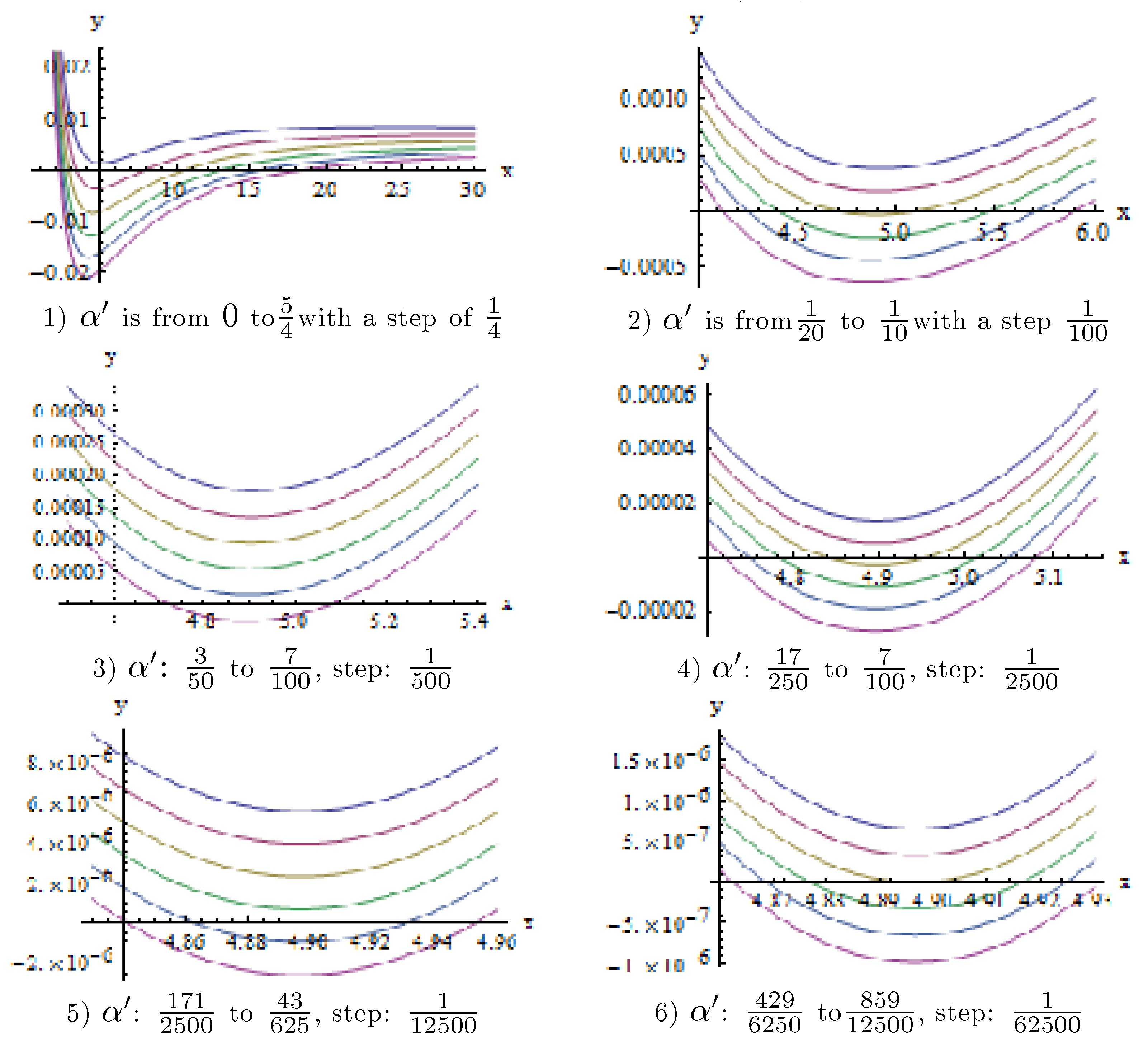
Now we get back to Equations (19) and (20) and use some internal functions of Mathematica and our algorithm to draw the graphs of $y=H^{\prime }(x,\alpha )$ for several values of ${\alpha }^{\prime }=\alpha -4$ and present them in Figure 2.

In these sets of graphs, the graph of $y=H^{\prime }(x,\alpha )$ moves down one curve as ${\alpha }^{\prime }$ increases one given step. From these figures, we can see that $H^{\prime }(x,\alpha )$ is above the x axis entirely and therefore the function $H(x,\alpha )$ increases monotonously on $(0,\infty )$ when $\alpha$ or ${\alpha }^{\prime }$ increases above some points. We can clearly see that the third curve ($\alpha =4.068672$) from the top of set (6) is almost tangent to the $x-$axis, based on which we may claim that ${\alpha }_0\approx 4.068672.$ For getting a clear view, we refine the graph of $y=H^{\prime }(x,\alpha )$ for the value of $\alpha$ between $4.06867220$ and $4.06867225$.

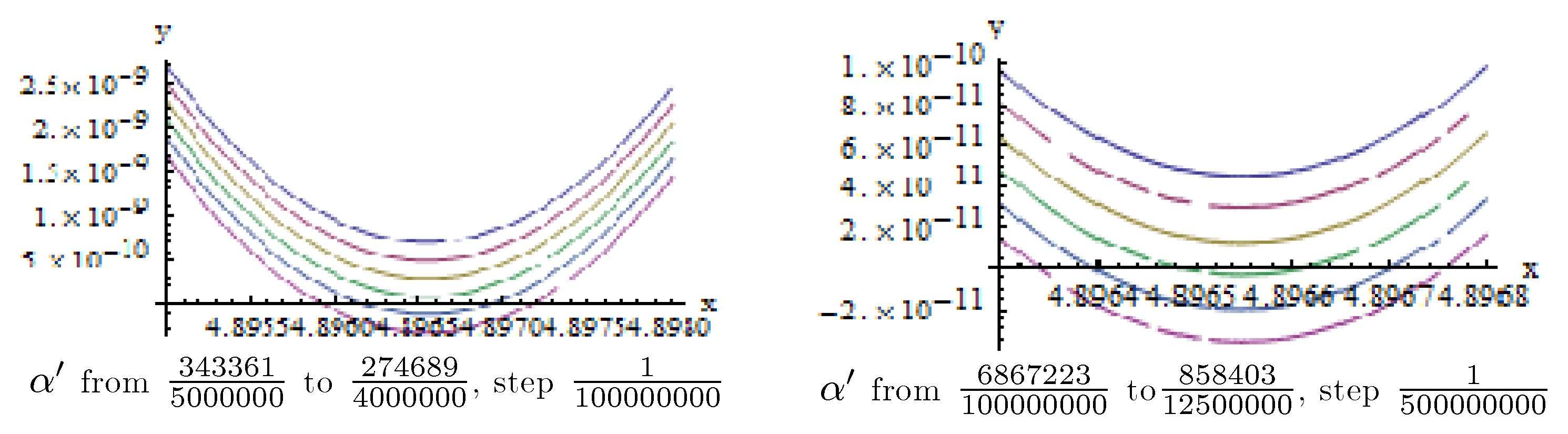
From the left set of Figure 3, one can clearly see that the second graph from the bottom intersects the x-axis, and the third graph is above the x-axis, which shows that $4.06867223<{\alpha }_0<4.06867224.$ The right set of Figure 3 shows that the third graph from the bottom intersects the x-axis, and the fourth curve is above the x-axis, which shows $4.0686722336<{\alpha }_0<4.0686722344.$ Now, we can conclude that the value of ${\alpha }_0$is between $4.0686722336$ and $4.0686722344$ for BVP (1) to have a unique solution when $0<\alpha \le {\alpha }_0$ and three solutions when ${\alpha }_0<\alpha <+\infty .$ As we have mentioned earlier, the distance between the three solutions is within $6.5\times {10}^{-14}$ even if there are three different solutions when the value of $\alpha$ is less than $4.0686722344.$ We can reasonably say that BVP (1) has a unique solution when $0<\alpha <4.0686722344$ for practical purposes.

5. Multiple Solution Region Determined by $\mathbf{\alpha }$ and $\mathbf{\lambda }$

When $\alpha >{\alpha }_0$ and $2H_{min}^2\left(\alpha \right)<\lambda <2H_{max}^2\left(\alpha \right),$ Equation (17) has three roots, and in turn BVP (1) has three solutions. We want to draw the curves of $2H_{min}^2\left(\alpha \right)$ and $2H_{max}^2\left(\alpha \right)$ by curve fitting for displaying the dependence of the values of $\alpha ,$${\lambda }_{*}$ and ${\lambda }^{*}$. Because the data in Table 1 are not enough for fitting these two curves, we use Mathematica language and our algorithm to generate more data in addition to those in Table 1, and record it in

Table 3. Extrema distribution of $H(x,\alpha )$ for $\alpha >5$.

$\mathit{\alpha }$	${\mathit{x}}_{\mathit{\alpha },1},\mathit{H}({\mathit{x}}_{\mathit{\alpha },1},\mathit{\alpha })$	${\mathit{x}}_{\mathit{\alpha },2},\mathit{H}({\mathit{x}}_{\mathit{\alpha },2},\mathit{\alpha })$
$\alpha =40$	1.25301760448467,0.67171261025458	${1863.6216520667076,1.5*10}^{-7}$
$\alpha =28$	1.28429966769793,0.67574695575337	890.7302648690519,0.0000425531142
$\alpha =22$	1.31449211684876,0.67952292381322	537.1422651607531,0.0006676773062
$\alpha =17$	1.35898307028123,0.68488600917206	310.133861485143,0.00623427026945
$\alpha =13$	1.42574378468659,0.69251111177893	172.787457627501,0.03482427254640
$\alpha =10$	1.52435591220294,0.70292524627786	95.5658692004087,0.11821275724685
$\alpha =8$	1.65400752694614,0.71524903451494	56.3243197953691,0.25248737845250
$\alpha =7$	1.76675466787322,0.724856688353225	40.3468564350250,0.35925984152783
$\alpha =6$	1.95576086475593,0.73897731600624	26.7542708531433,0.49770116722831

below.

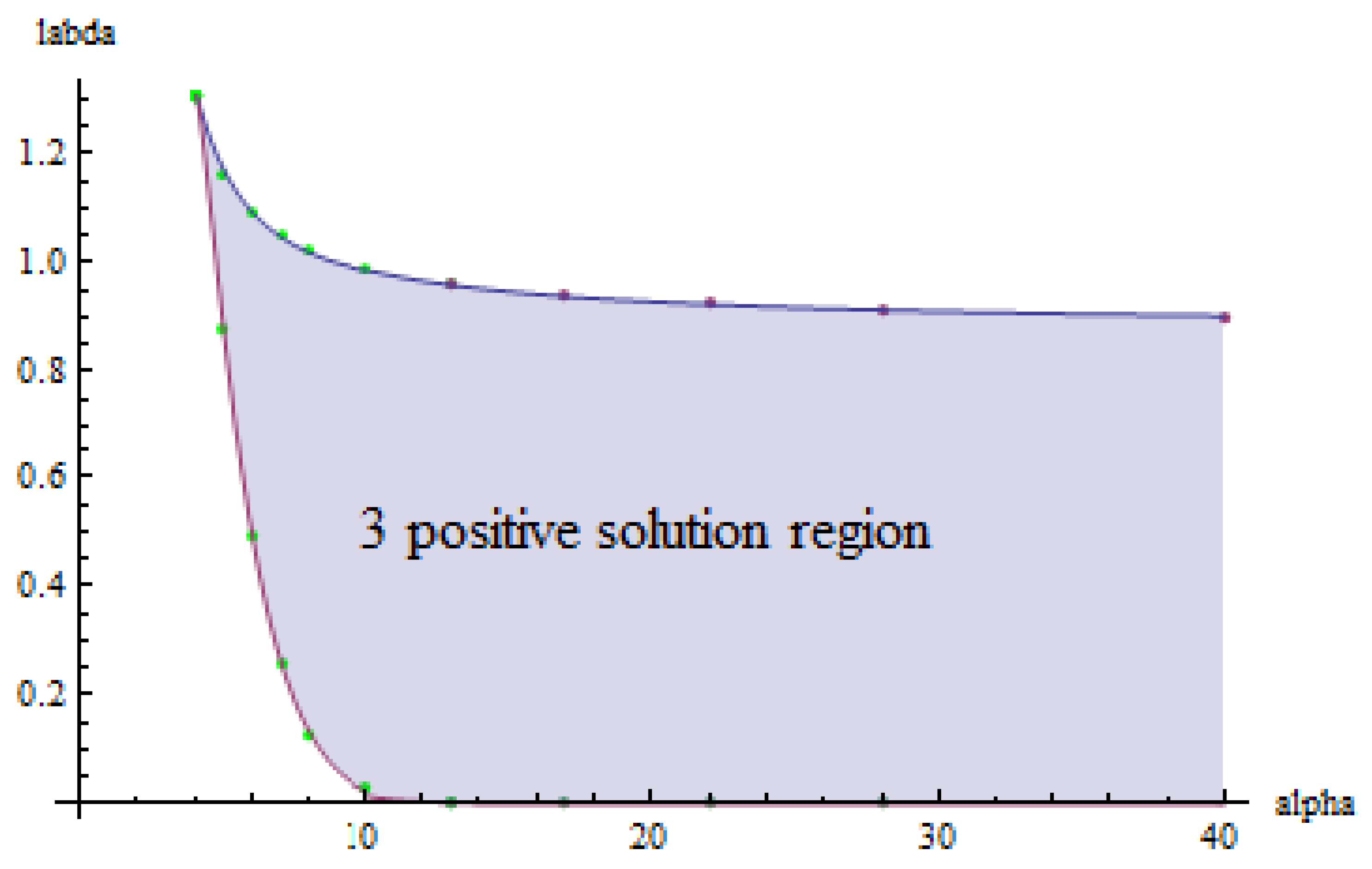
Using some internal functions of Mathematica and the data in Table 1 and Table 3, the curves of $\lambda =2H_{max}^2\left(\alpha \right)$ and $\lambda =2H_{min}^2\left(\alpha \right)$ are fitted out in Figure 4, where

$$\begin{array}{c}\lambda =2H_{max}^2\left(\alpha \right)=\left\{\begin{array}{c}0.948687+\frac{7.44803}{{\alpha }^2}-\frac{0.374545}{\alpha },0<\alpha <10\hfill \\ 0.878865+\frac{1.96024}{{\alpha }^2}+\frac{0.892728}{\alpha },\alpha \ge 10\hfill \end{array}\right.\end{array}\left(31\right)$$

(31)

and

$$\begin{array}{c}\lambda =2H_{min}^2\left(\alpha \right)=\left\{\begin{array}{c}0.159105-\frac{2012.94}{{\alpha }^4}+\frac{920.173}{{\alpha }^3}-\frac{85.7181}{{\alpha }^2}+\frac{0.0399875}{\alpha },0<\alpha <10\hfill \\ -0.0036898+\frac{609.536}{{\alpha }^4}-\frac{42.5637}{{\alpha }^3}+\frac{1.84242}{{\alpha }^2}+\frac{0.195639}{\alpha },10\le \alpha \le 40\hfill \\ 0,\alpha >40\hfill \end{array}\right..\end{array}\left(32\right)$$

(32)

Figure 4 shows a clear relationship of the values of $\alpha$ and $\lambda$ for BVP (1) to have three solutions.

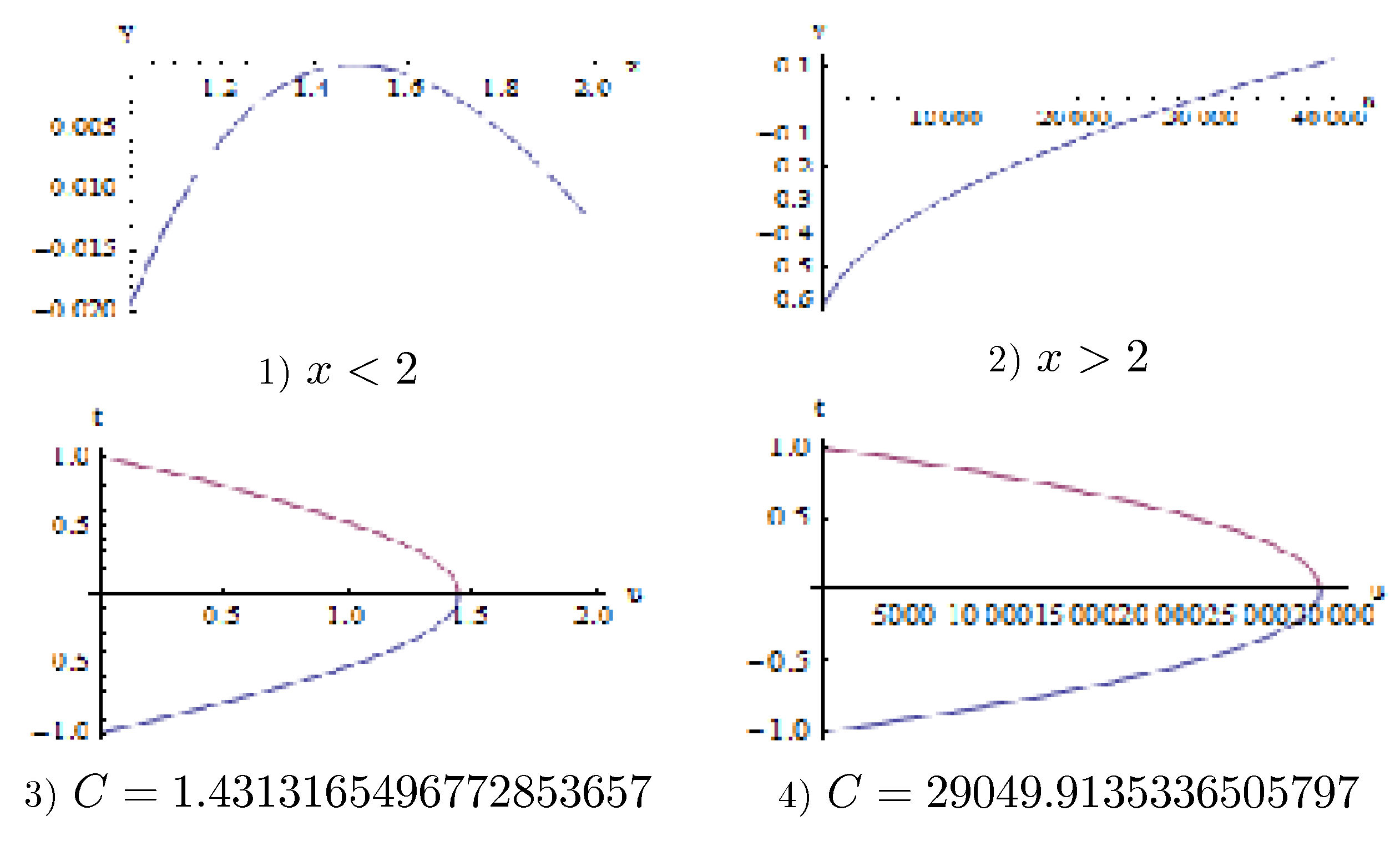
When $\alpha >{\alpha }_0,$$\lambda <2H_{min}^2\left(\alpha \right)$or $\lambda >2H_{max}^2\left(\alpha \right),$ Equation (17) has only one root, thus BVP (1) has a unique solution. When $\alpha >{\alpha }_0,$$\lambda =2H_{min}^2\left(\alpha \right)$or $\lambda =2H_{max}^2\left(\alpha \right),$ Equation (17) has two roots, thus BVP (1) has two solutions. Now, we try to graph the two solutions corresponding to some values of $\lambda$ and $\alpha .$

Let $\alpha =11,\lambda =2H_{max}^2\left(11\right)\approx 0.69854478,$the two roots of Equation (17) are $C_1=1.4313165496772853657$ and $C_2=29048.91353365085797.$ Using the values of $C_1$and $C_2,$ we get the corresponding solutions of BVP (1) using (26). Their images are shown in Figure 5 with the corresponding graph of $y=H(x,\alpha )-\sqrt{\frac{\lambda }{2}}$ above them.

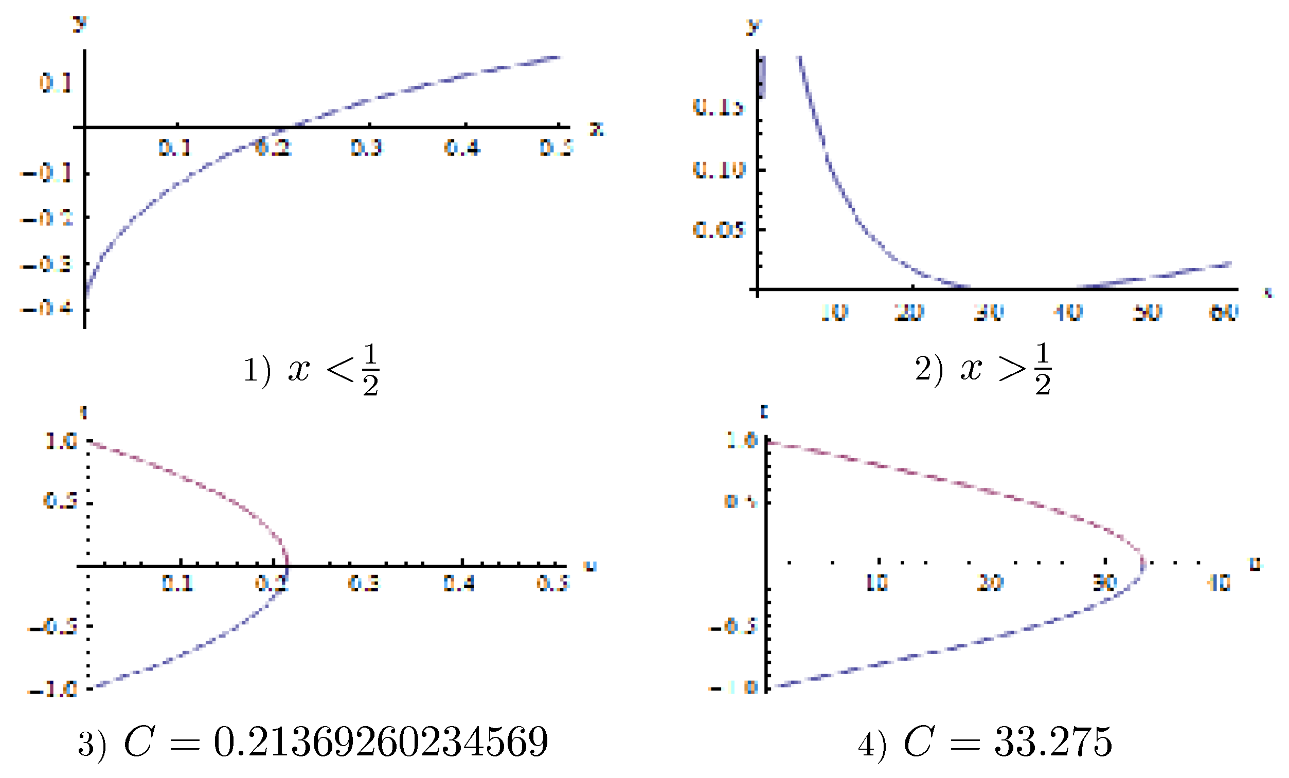
Let $\alpha =6.5,\lambda =2H_{max}^2\left(6.5\right)\approx 0.35941826,$the two roots of Equation (17) are $C_1=0.21369260234569$ and $C_2=33.275.$ Using these values of $C_1$and $C_2,$ we get the corresponding two solutions of BVP (1) using (26). Their images are shown in Figure 6 with the corresponding graph of $y=H(x,\alpha )-\sqrt{\frac{\lambda }{2}}$ above them.

It can be seen from (2) in Figure 6 that the function $y=H[x,\alpha )-\sqrt{\frac{\lambda }{2}}$ changes gently near the minimum point. If $\lambda$ deviates slightly, it will enter the three positive solution region or the unique solution region. Therefore, it is quite challenging to find two positive solutions in the lower boundary of the three positive solution region.

6. Conclusions

In this article, we studied the well-known one-dimensional perturbed Gelfand two-point boundary value problem (1). We first converted it to equivalent integral representation (11). By reducing (11) to a single integral and combining Newton’s method with the dichotomy method, we developed a very efficient algorithm with high precision for computing the values of ${\alpha }_0,{\lambda }_{*}$ and ${\lambda }^{*}$ such that this problem has a unique solution when $0<\alpha <{\alpha }_0$ and $\lambda >0,$ and has three solutions when $\alpha >{\alpha }_0$ and ${\lambda }_{*}<\lambda <{\lambda }^{*}.$ Our result improves the the existing result by Huang and Wang [8,9] from ${\alpha }_0\approx$$4.069$ to ${\alpha }_0\approx 4.0686722336.$This improvement of approximation is essential for finding the exact value of ${\alpha }_0$ in future works. We also used a separate section to prove that there is a positive number $ϵ$ such that BVP (1) has a unique solution for all values of $\lambda >0$ and $\alpha \in (0,4+ϵ).$ Once the value of ${\alpha }_0$ is found, finding the values of ${\lambda }_{*}$ and ${\lambda }^{*}$ becomes necessary. We used our algorithm to approximate these values with accuracy up to ${10}^{-14}$ corresponding to a few values of ${\alpha }_0.$ A region illustrating the dependence of the values of $\alpha ,{\lambda }_{*}$ and ${\lambda }^{*}$ is graphed. Hopefully, this pattern of dependence can help future researchers to figure out the precise dependence of these values. During the revision process of this article, we have noticed that the method of optimal fourth order multiple root solvers without using derivatives developed by Sharma, Kumar and Jäntschi [16] may be applied to this problem. We will certainly explore this alternate route and try to improve our result further in our future work.