
Qualitative Theory of Two-Dimensional Polynomial Dynamical Systems

Abstract
:1. Introduction
2. Autonomous Polynomial Dynamical Systems
2.1. Classification of Autonomous Polynomial Dynamical Systems
2.2. On Integrability of Polynomial Dynamical Systems
2.3. Symmetries of Quadratic Polynomial DSs
2.4. Extension to Higher-Degree Polynomials
3. Classes D of Solutions to Quadratic Polynomial DSs. Discriminant Criterion. Linearization
3.1. Discriminant Criterion
- (1)
- D: and
- (2)
- D: and
- (3)
- D: and
- (4)
- D: and
3.2. Linearization in D
3.3. Analysis of Solutions to Cauchy Problems
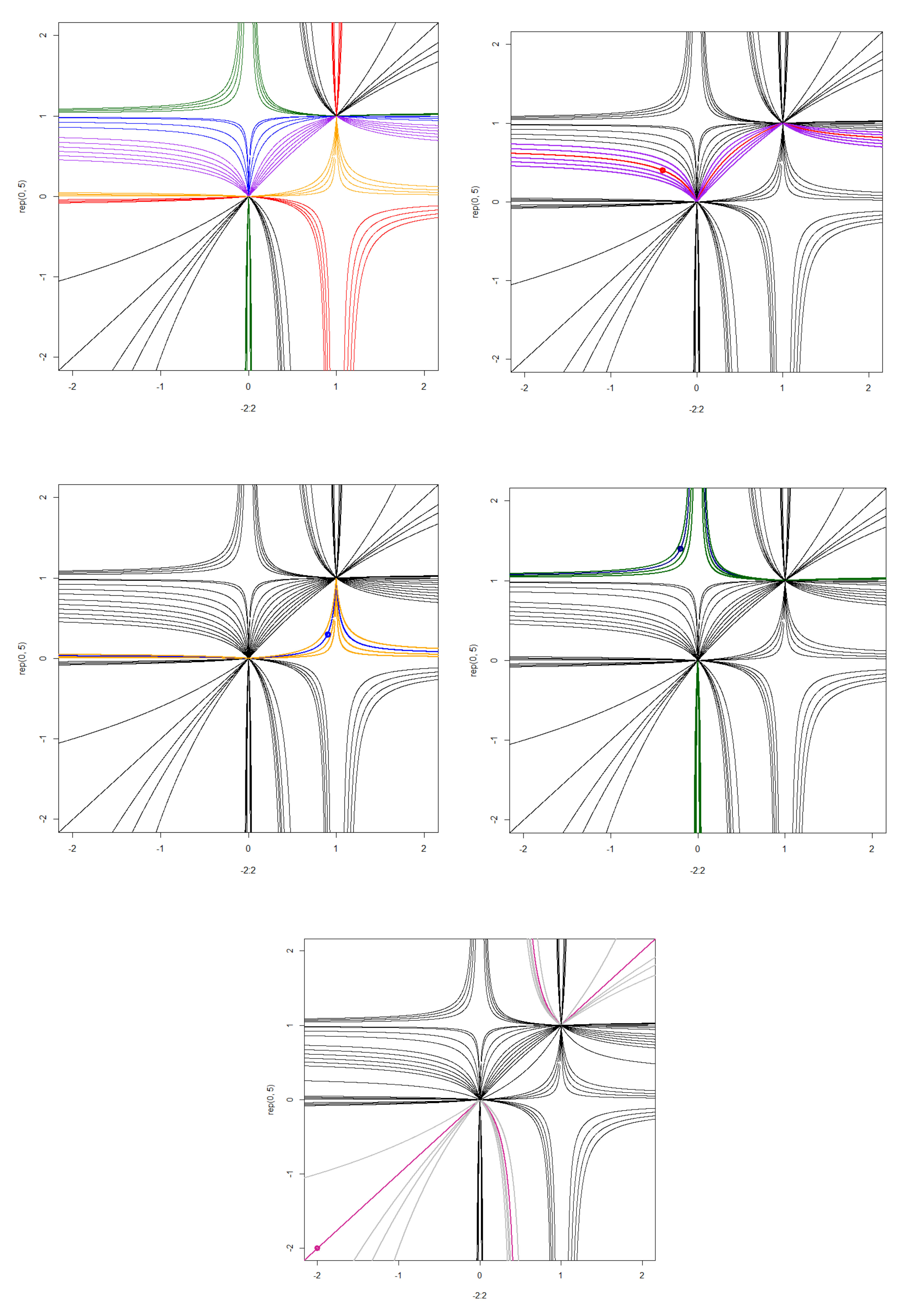
- at any increases at and decreases at (black lines in Figure 3);
- at any decreases at increases at, and is situated in the band between and (blue lines in Figure 3);
- for increases at, decreases at , and is situated outside (green lines in Figure 3);
- at any decreases at increases at , and is situated in (magenta lines in Figure 3);
- at any decreases at increases at , and is situated outside (red lines in Figure 3);
- at increases at decreases at , and is situated in (orange lines in Figure 3).
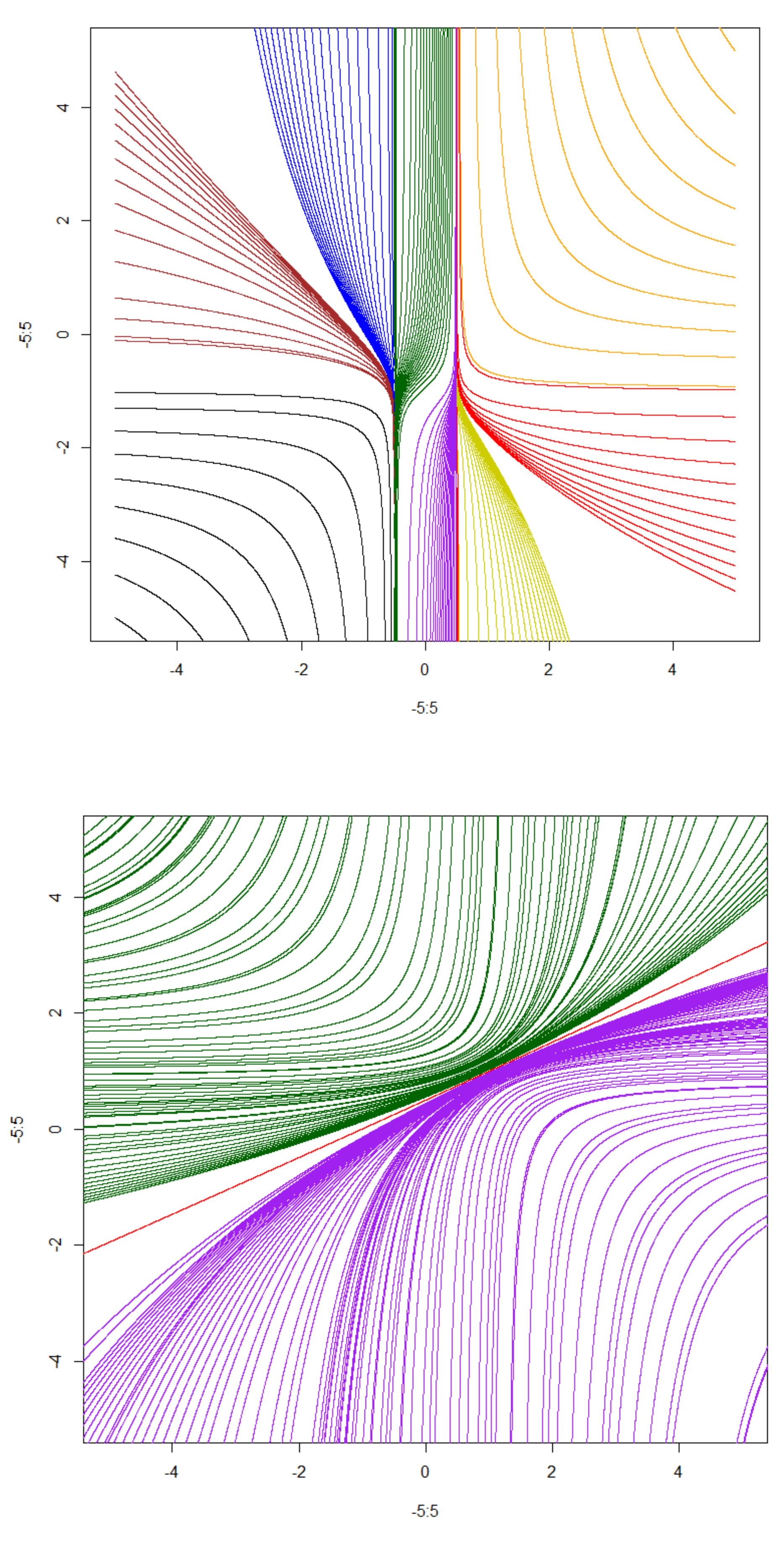
- (a)
- for and any the solutions are monotonically increasing functions that lie in the strip between two special stationary solutions and
- (b)
- for or and any the solutions are monotonically decreasing unbounded functions that lie outside the strip between two stationary solutions. In the considered case, the entire phase plane is filled with the solution curves.
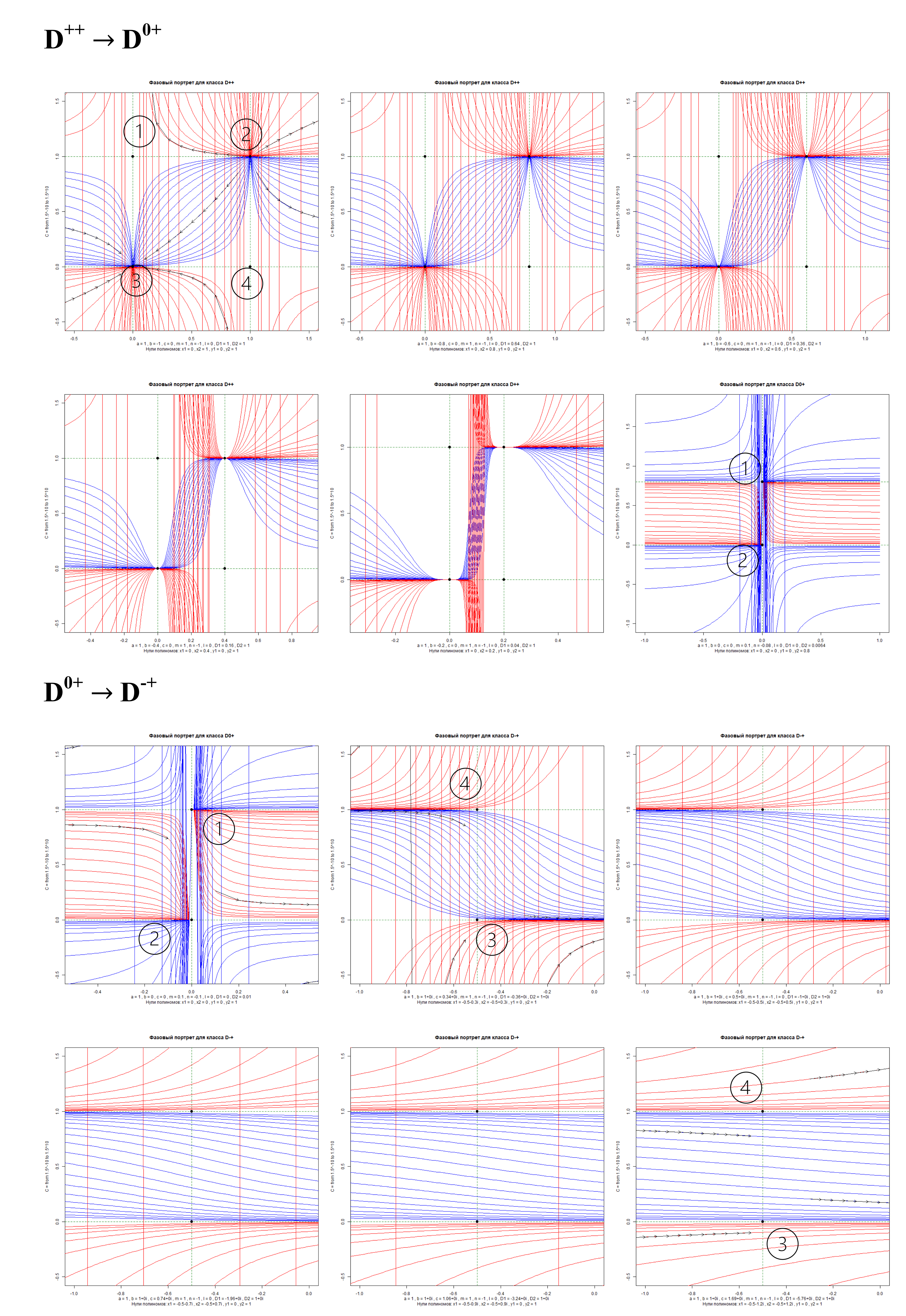
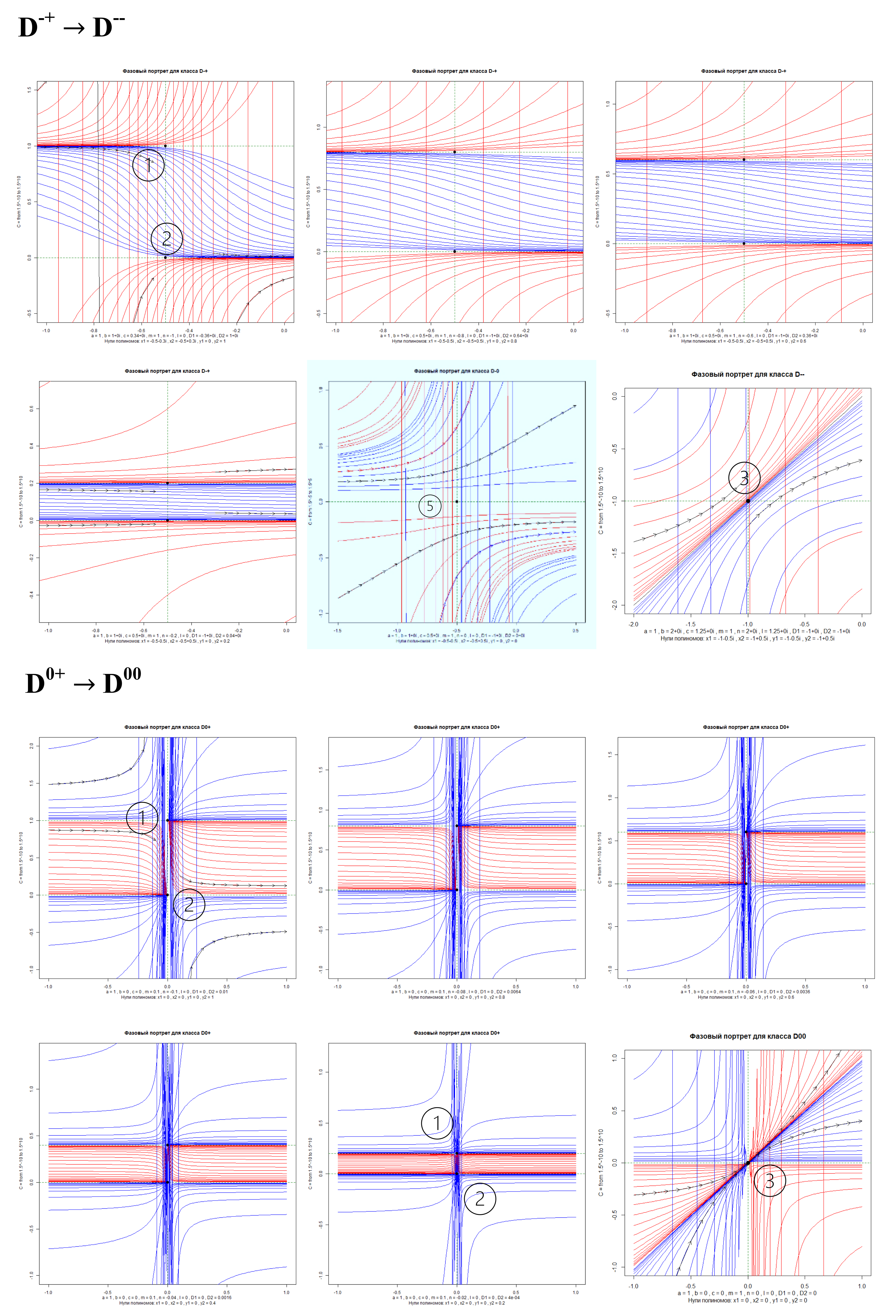
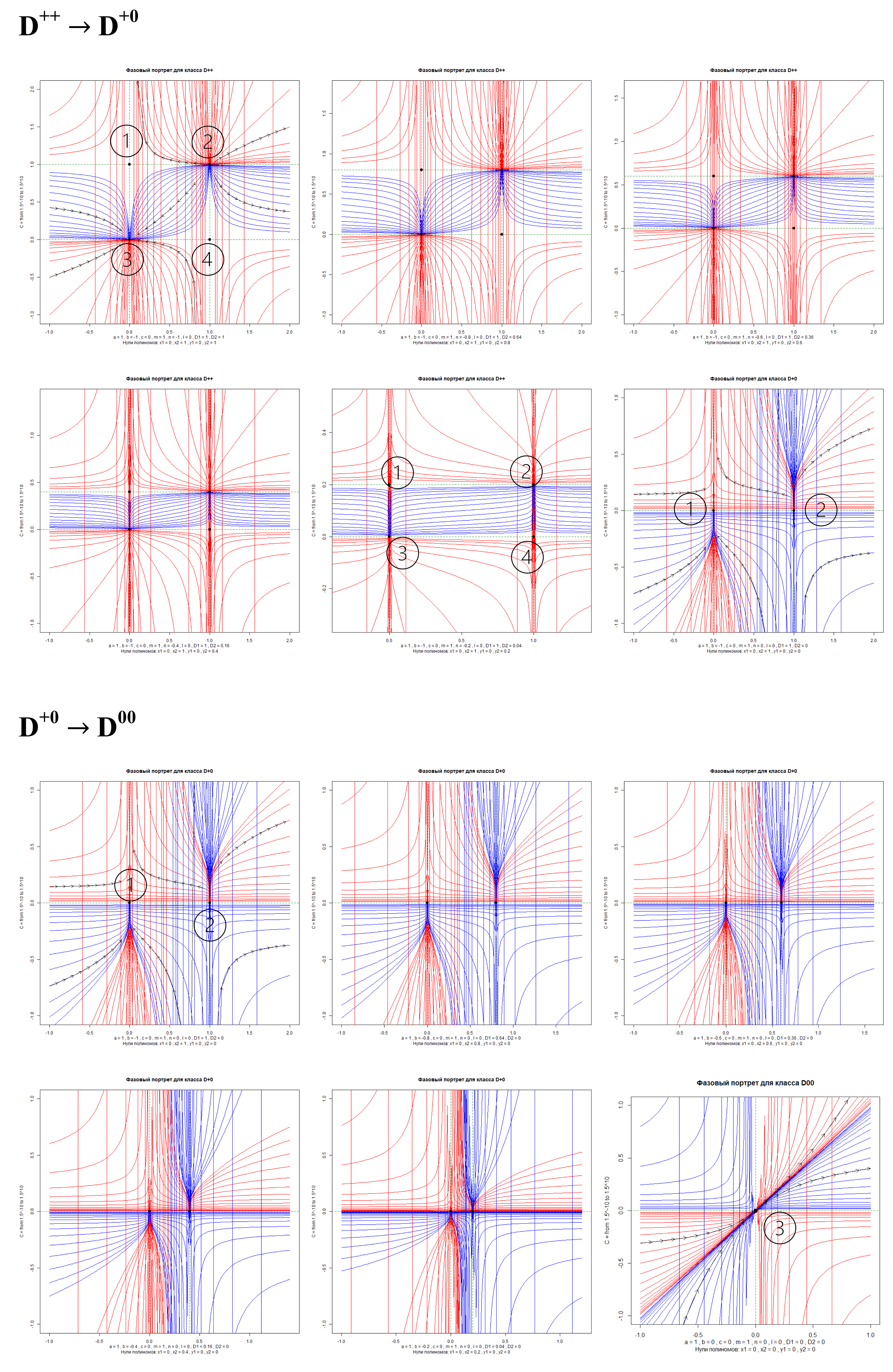
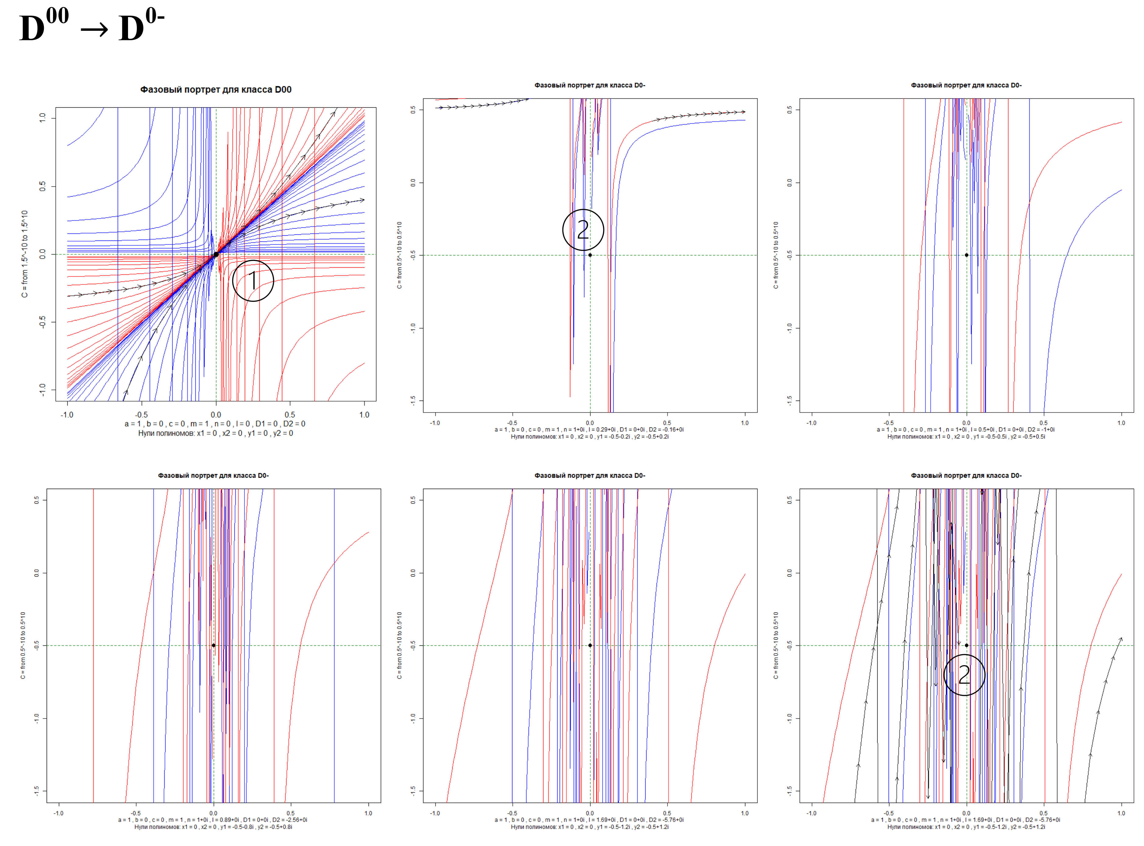
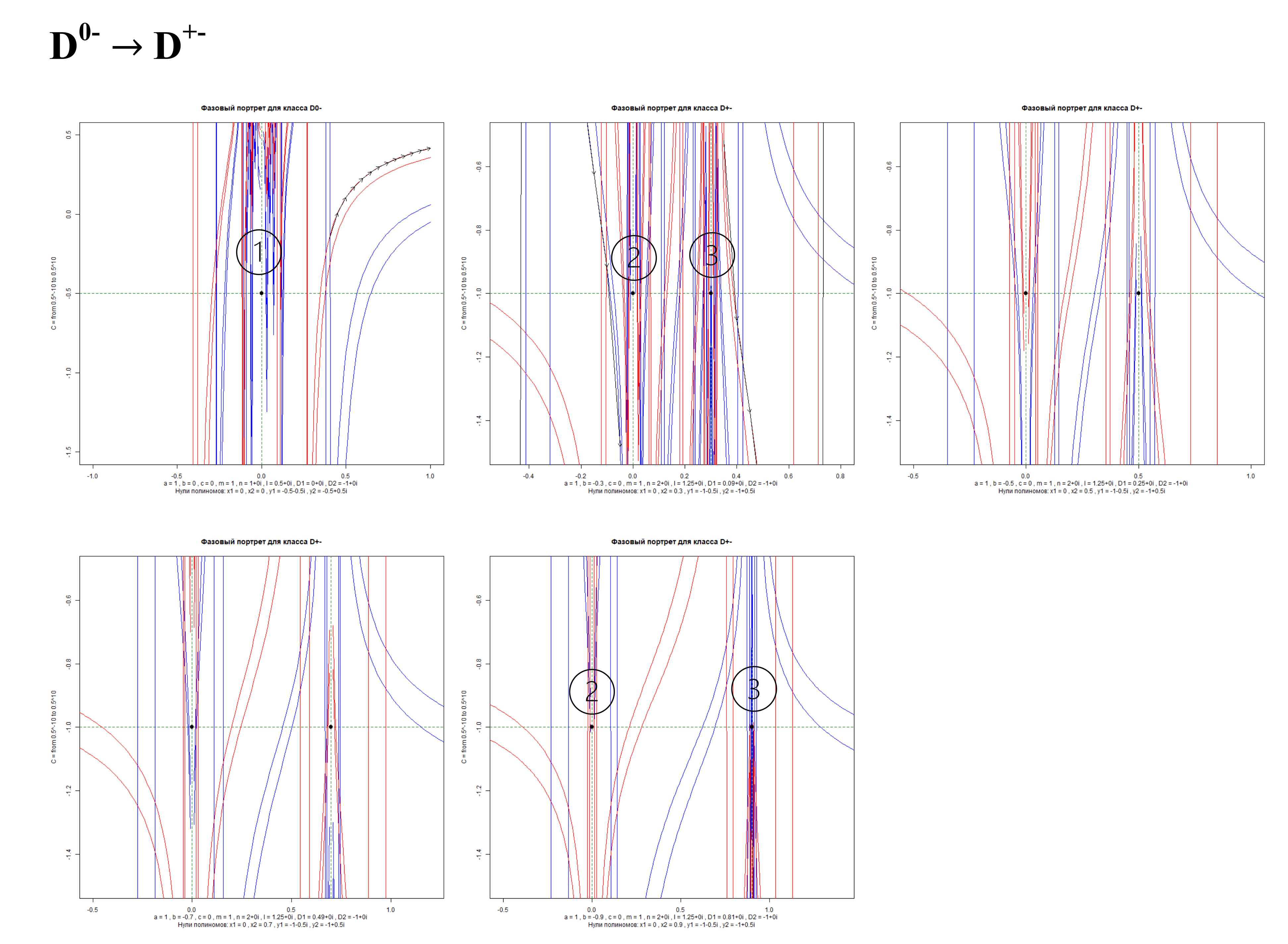
4. Qualitative Theory of Polynomial Quadratic DSs. Visualization of Transitions
4.1. Analysis of Solutions and Phase Portraits
4.2. Atlas of Phase Portraits
5. Conclusions
Author Contributions
Funding
Institutional Review Board Statement
Informed Consent Statement
Conflicts of Interest
References
- Abraham, R.H.; Shaw, C.D. Dynamics—The Geometry of Behavior; Addison-Wesley: Boston, MA, USA, 1992. [Google Scholar]
- Arrowsmith, D.K.; Place, C.A. An Introduction to Dynamical Systems; Cambridge University Press: Cambridge, UK, 1990. [Google Scholar]
- Anatoliy, G. Butkovskiy, Phase Portraits of Control Dynamical Systems; Kluwer Academic Publishers: Dordrecht, The Netherlands, 1991. [Google Scholar]
- Brodlie, K.W.; Carpenter, L.A.; Earnshaw, R.A.; Gallop, J.R.; Hubbold, R.J.; Mumford, A.M.; Osland, C.D.; Quarendon, P. (Eds.) Scientific Visualization—Techniques and Applications; Springer: Berlin/Heidelberg, Germany, 1992. [Google Scholar]
- Thomson, J.M.T. Instabilities and Catastrophes in Science and Engineering; John Wiley & Sons: New York, NY, USA, 1982. [Google Scholar]
- Brenig, L. New special functions solving nonlinear autonomous dynamical systems. arXiv 2009, arXiv:0910.2584v1. [Google Scholar]
- Brenig, L.; Goriely, A. Universal canonical forms for time-continuous dynamical systems. Phys. Rev. A 1989, 40, 4119–4125. [Google Scholar] [CrossRef] [PubMed]
- Yu, E.; Bun’kova, V.M. Bukhshtaber, Polynomial dynamical systems and ordinary differential equations associated with the heat equation. Funct. Anal. Appl. 2012, 46, 173–190. [Google Scholar]
- Kondratyeva, Y.V. Two-Dimensional Polynomial Dynamical Systems with Algebraically Invariant Sets; Differentsial’nye Uravnenija: Nizhnij Novgorod, Russia, 2006. (In Russian) [Google Scholar]
- Gaiko, V.A. On global bifurcations and Hilbert’s sixteenth problem. Nonlinear Phenom. Complex Syst. 2000, 3, 11–27. [Google Scholar]
- Shakhverdive, A.Kh.; Shestopalov, Y.V. Qualitative Analysis of Quadratic Polynomial Dynamical Systems Associated with the Modeling and Monitoring of Oil Fields. Lobachevskii J. Math. 2019, 40, 1691–1706. [Google Scholar] [CrossRef]
- Chossat, P.; Lauterbach, R. Methods in Equivariant Bifurcations and Dynamical Systems; World Scientific: Singapore, 2000. [Google Scholar]
- Murdock, J. Normal Forms and Unfoldings for Local Dynamical Systems; Springer: New York, NY, USA, 2003. [Google Scholar]
- Nicolis, G. Prigogine, I. Self-Organization in Non-Equilibrium Systems. From Dissipative Structures to Order through Fluctuations; John Wiley & Sons: New York, NY, USA, 1977. [Google Scholar]
- Buckley, S.E.; Leverett, M.C. Mechanism of Fluid Displacement in Sands. Trans. AIME 1942, 146, 107. [Google Scholar] [CrossRef]
- Shakhverdiev, K. System Optimization of Oil Field Development Processes; Nedra: Moscow, Russia, 2004. (In Russian) [Google Scholar]
- Shakhverdiev, A.K. System optimization of non-stationary waterflooding for IOR/EOR. Neft. Khozjaistvo 2019, 1, 44–50. [Google Scholar]
- Ahmad, S.; Ambrosetti, A. A Textbook on Ordinary Differential Equations, 2nd ed.; Springer: Berlin/Heidelberg, Germany, 2015. [Google Scholar] [CrossRef]

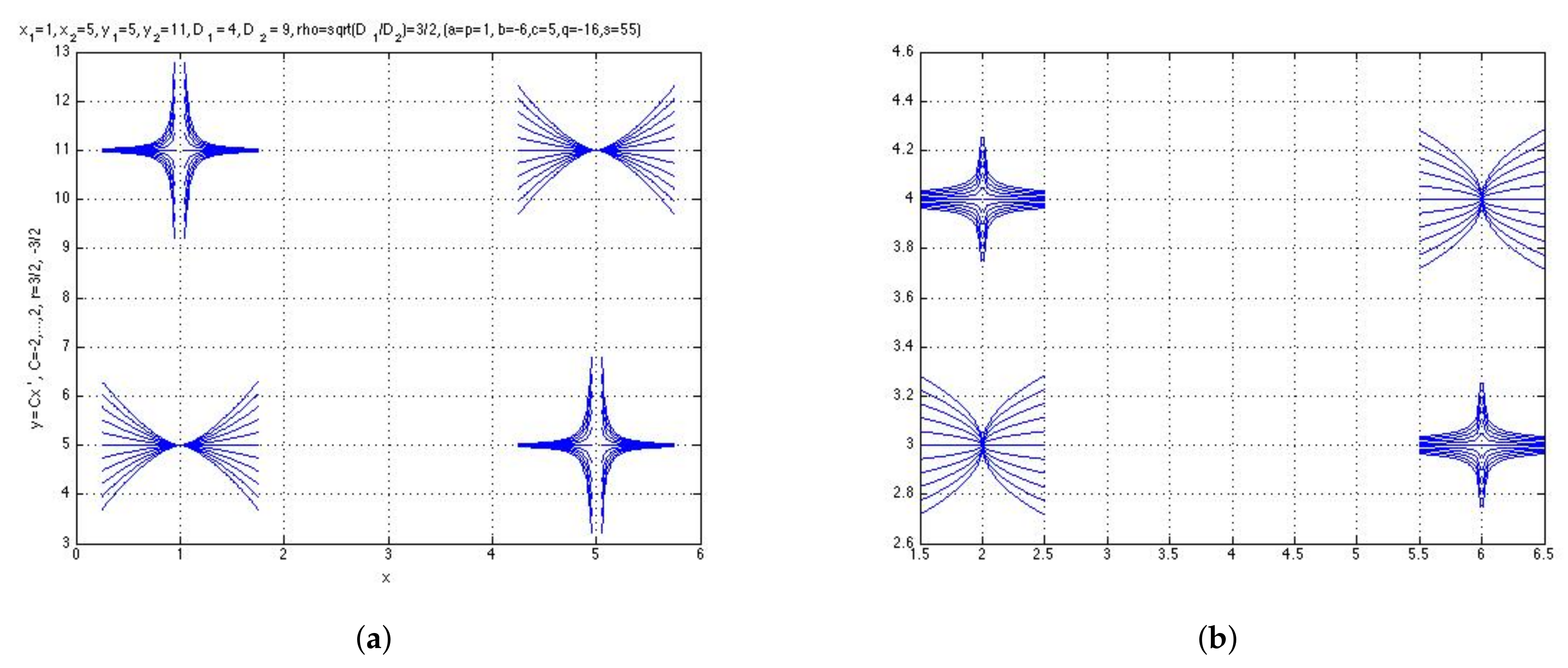
| (a) | (b) |


| Class | Example of Equation | General Solutions of | |
|---|---|---|---|
| 1 | D | , | |
| 2 | D | ||
| 3 | D | ||
| 4 | D | ||
| 5 | D | ||
| 6 | D | ||
| 7 | D | , , | |
| 8 | D | , | |
| 9 | D |
| Stable Node | Unstable Node | Saddle | |
|---|---|---|---|
| Stable Node | |||
| Unstable Node | |||
| Saddle |
Publisher’s Note: MDPI stays neutral with regard to jurisdictional claims in published maps and institutional affiliations. |
© 2021 by the authors. Licensee MDPI, Basel, Switzerland. This article is an open access article distributed under the terms and conditions of the Creative Commons Attribution (CC BY) license (https://creativecommons.org/licenses/by/4.0/).
Share and Cite
Shestopalov, Y.; Shakhverdiev, A. Qualitative Theory of Two-Dimensional Polynomial Dynamical Systems. Symmetry 2021, 13, 1884. https://doi.org/10.3390/sym13101884
Shestopalov Y, Shakhverdiev A. Qualitative Theory of Two-Dimensional Polynomial Dynamical Systems. Symmetry. 2021; 13(10):1884. https://doi.org/10.3390/sym13101884
Chicago/Turabian StyleShestopalov, Yury, and Azizaga Shakhverdiev. 2021. "Qualitative Theory of Two-Dimensional Polynomial Dynamical Systems" Symmetry 13, no. 10: 1884. https://doi.org/10.3390/sym13101884