
A New Constructive Method for Solving the Schrödinger Equation


Institute of Computer Science, Pedagogical University of Krakow, Podchorążych 2, 30-084 Kraków, Poland
Symmetry 2021, 13(10), 1879; https://doi.org/10.3390/sym13101879
Submission received: 3 September 2021
/
Revised: 29 September 2021
/
Accepted: 1 October 2021
/
Published: 5 October 2021
(This article belongs to the Special Issue Symmetry and Approximation Methods)
Abstract
:In this paper, a new method for the exact solution of the stationary, one-dimensional Schrödinger equation is proposed. Application of the method leads to a three-parametric family of exact solutions, previously known only in the limiting cases. The method is based on solutions of the Ricatti equation in the form of a quadratic function with three parameters. The logarithmic derivative of the wave function transforms the Schrödinger equation to the Ricatti equation with arbitrary potential. The Ricatti equation is solved by exploiting the particular symmetry, where a family of discrete transformations preserves the original form of the equation. The method is applied to a one-dimensional Schrödinger equation with a bound states spectrum. By extending the results of the Ricatti equation to the Schrödinger equation the three-parametric solutions for wave functions and energy spectrum are obtained. This three-parametric family of exact solutions is defined on compact support, as well as on the whole real axis in the limiting case, and corresponds to a uniquely defined form of potential. Celebrated exactly solvable cases of special potentials like harmonic oscillator potential, Coulomb potential, infinite square well potential with corresponding energy spectrum and wave functions follow from the general form by appropriate selection of parameters values. The first two of these potentials with corresponding solutions, which are defined on the whole axis and half axis respectively, are achieved by taking the limit of general three-parametric solutions, where one of the parameters approaches a certain, well-defined value.
1. Introduction
One of the main open problems in nonrelativistic quantum mechanics is finding exact bound states to microscopic systems. The early attempts concerned the energy spectrum of the hydrogen atom and were successfully concluded using the Bohr-Sommerfeld quantization rule [1]. The introduction of the Schrödinger equation enabled the application of the theory of orthogonal polynomials to the bound state problem.
Over the years, new techniques have been introduced [2,3], like algebraic methods connected with annihilation and creation operators or the factorization method introduced by Infeld and Hull [4,5,6]. Using supersymmetry [7,8], another method was proposed, namely the so-called shape invariance condition [9,10,11], which is an integrability condition generalizing the operator method employed for solving the harmonic oscillator. Shape invariance allowed to find new exact solutions [12,13,14,15,16], as well as gave a novel insight into the problem of solvability of the Schrödinger equation. In particular, all the popular analytically solvable potentials, such as harmonic oscillator potential, Coulomb potential, and infinite square well potential are known to be solvable using this method [12]. Furthermore, the shape invariance condition provides an answer to the question whether WKB and SWKB approximations methods are exact [17].
Exact solutions of the Schrödinger equation are widely researched also for their applications [18]. As an example, study of the deformations to exactly solvable potentials is facilitated by the existence of analytical solutions [19]. A comprehensive book by Bagrov and Gitman discusses several methods used to find exact solutions in nonrelativistic and relativistic quantum mechanics [20].
This paper introduces a three-parametric family of potentials that encompasses, as special cases, all of the potentials mentioned in the previous paragraph. The considered method uses the Ricatti equation to obtain a general set of solutions, that in the limiting cases is transformed into the known solutions by taking the appropriate values of parameters.
Solving the Schrödinger equation through the Ricatti equation is popular. Ricatti equation was also used to find approximations to the stationary Schrödinger equation [18,21]. Here, a new formalism is proposed where all so different solutions, like the ones mentioned above, emerge from a unique form of the potential, that admits parametrization by three real numbers.
The methods to solve the Schrödinger equation using continued fractions are utilized since the 1970s [22,23]. In this contribution, continued fractions are used to solve the general form of the potential and allow one to find the exact solutions of the Schrödinger equation simultaneously, which previously was obtained only in the special, isolated cases [24]. It is conjectured that all of the potentials that can be solved using orthogonal polynomials are special cases of this three-parametric family and can be therefore obtained employing the presented method.
2. The Ricatti Equation
One of the most interesting nonlinear differential equations of the first order is the Ricatti equation, which is applied in many different branches of mathematics and physics [28]. The general form of the Ricatti equation is:
where , , and are continuous functions of x. The scope of this paper is restricted to constant real functions , , and , which simplifies the Ricatti equation to the following form
The symbol refers to a function called in the other papers as superpotential.
2.1. Solutions to Special Ricatti Equation
The solution of this equation is sought in the compact interval I, while the conditions
are satisfied.
For unspecified constant of integration , Equation (2) admits the following solution
with compact support I given by
The main goal of this section is to find all solutions and positive parameters of the following family of equations for
having the solution as the initial function, determined by the real parameters A, B, and C. In the following reasoning, W with lower indices denote functions on the support I.
The solution of Equation (6) for is written by means of the initial function
which transforms Equation (6) to
This equation has the form of the Ricatti equation, given by Equation (2), if the unknown function is linear in
Then, using the linearity of , Equation (8) can be transformed to the form of Equation (2), producing the coefficients , , and
Extending the above notation to the case of one notes that , , and yields with (6) transformed into an identity equation. To find the next solution of the Equation (6), it is crucial to postulate the following form
with the function defined by the already found function and the unknown function with a real parameter .
Similar to the previous case, using the above assumptions concerning , from Equation (6) one obtains
Proceeding as before, the postulate that is linear in ,
transforms Equation (12) into the form of the Ricatti Equation (2), allowing to obtain the coefficients , , and . Furthermore, one immediately gets .
The general form of the results is further illustrated by the next solution,
while assuming that is linear in with real parameters and . The coefficients of the above solution and can be deduced using similar differential equation to (12)
In general, the solution is derived, by analogy, in iterative reasoning and reads
where the coefficients and of the auxiliary function can be determined from the differential equation
assuming is linear in the initial function . The real coefficient is also inferred from the above equation.
2.2. Coefficients of the Continued Fraction
The symmetry of Equation (16) is striking, with the real coefficients forming consecutive terms in the continued fraction. That is true even for the numerator, where is simply equal to zero. Using Equation (17) for to accomplish the values of coefficients and , one gets the solution of and the recursive equations for and , where
Solutions of the above recursive equations can be written as
with initial parameters , , and .
3. The Schrödinger and the Ricatti Equations
The time-independent Schrödinger equation is used throughout quantum physics, in particular, to find the bound states of various microscopic systems. Its one-dimensional version describes the complex amplitude of the n-th wavefunction that has the energy in the presence of the potential
where .
The wavefunction is used to determine the density of probability of finding a particle in the position x, given by the Born rule . Since it describes the physical reality its normalizability is required, and the wavefunctions of different energy are orthogonal over the support
where is a positive real value.
This section shall be devoted to solving the Schrödinger equation by transforming it into the Ricatti equation via the logarithmic derivative , which produces
The normalizability condition of the wavefunction results in the positivity of the derivative , which implies the existence of the inverse function in the region I. Then, the crucial step is the transformation of the function into a variable by .
Therefore, a new form of Equation (22) for is obtained
where the notation denotes a function depending on variable . Restricting to the case of f quadratic in transforms the above equation into
described by three real parameters A, B, and C.
Taking into account the common potential for all solutions , one eliminates it from the general solution to the Schrödinger Equation (22), which takes the form of
Note that this equation has identical form to Equation (6), where , while the initial function admits the starting condition for the superpotential (2). Thus, the procedure explained in the previous section may be used for finding all solutions .
Now, as a final step for acquiring the wavefunctions of the first bound state, the solution to the Ricatti equation is integrated and exponentiated, resulting in
where A, B, and C are real parameters that encode the wavefunction implicit dependence on the potential. For simplicity, the constants of two integrations are not included.
Similarly, for one gets -4.6cm0cm
The general solution reads
where all coefficients written in Greek letters depend on the A, B, and C parameters and must be determined by a cumbersome integration of for each bound state separately. Analytical and numerical calculations suggest that the functions are orthogonal and normalizable, , which is additional proof of correctness of the procedure.
Based on the previously found expression of and the Schrödinger Equation (22), it is possible to evaluate the general form of the three-parametric potential V in the variable
Note that the starting Equation (2) has three parameters A, B, and C, while its solution has an additional one . The above formula admits bound states only if the potential opens upwards, i.e. tends to infinity at the boundaries of the domain I. Therefore, the trigonometric potentials are obtained using the following condition
The hyperbolic potentials, such as the Morse potential, are obtained by a complementary constraint on the parameters,
Finally, the energies of the bound states are given by a simple relation
and, for excited states,
The above concludes the considerations of the general form of the Schrödinger Equation (22), quadratic in . The abundance of the solutions that use orthogonal polynomials makes it unfeasible to check every one of them. Nonetheless, to convince the reader that the exhibited method is comprehensive, the next section is focused on its connection to three well-known examples via a proper choice of parameters.
4. Examples of Potentials
This section shall be devoted to the study of specific examples of trigonometric potentials arising from the careful choice of parameters. Both relationships (29) and (33) between the potential/energy and the parameters A, B and C respectively, can be used to adjust the parameters in order to obtain known potentials.
However, in this contribution, the equation for energy will be used, where the dependence on n is three-fold: linear n, quadratic , or inverse quadratic . Each corresponds to a different, solvable potential: harmonic oscillator, infinite square well potential, and the Coulomb potential, respectively.
4.1. Infinite Square Well Potential
For instance, if one takes , , and , then the Schrödinger equation for the infinite square well potential is acquired. The solutions, resulting from Equations (26)–(28) and (33) that are dedicated to the wavefunctions and energy spectrum, read
where and energy . Alternatively, this solution can be obtained by the continued fraction (16). This example is generally considered to be the simplest solution of the Schrödinger equation and, in the case at hand, was achieved by the special choice of all three parameters together.
4.2. Harmonic Oscillator Potential
The next example is related to the harmonic oscillator potential. The choice and is made while, to simplify calculations, . From the general expressions (26) and (27) for the ground state and the first excited state one obtains
where , and energy .
The exact expression for the second excited state can be evaluated using the continued fraction (16)
By analogy, this scheme can be applied to the higher excited states as well. In addition, to simplify the limiting procedure, every denominator of the function included the constant of integration equal .
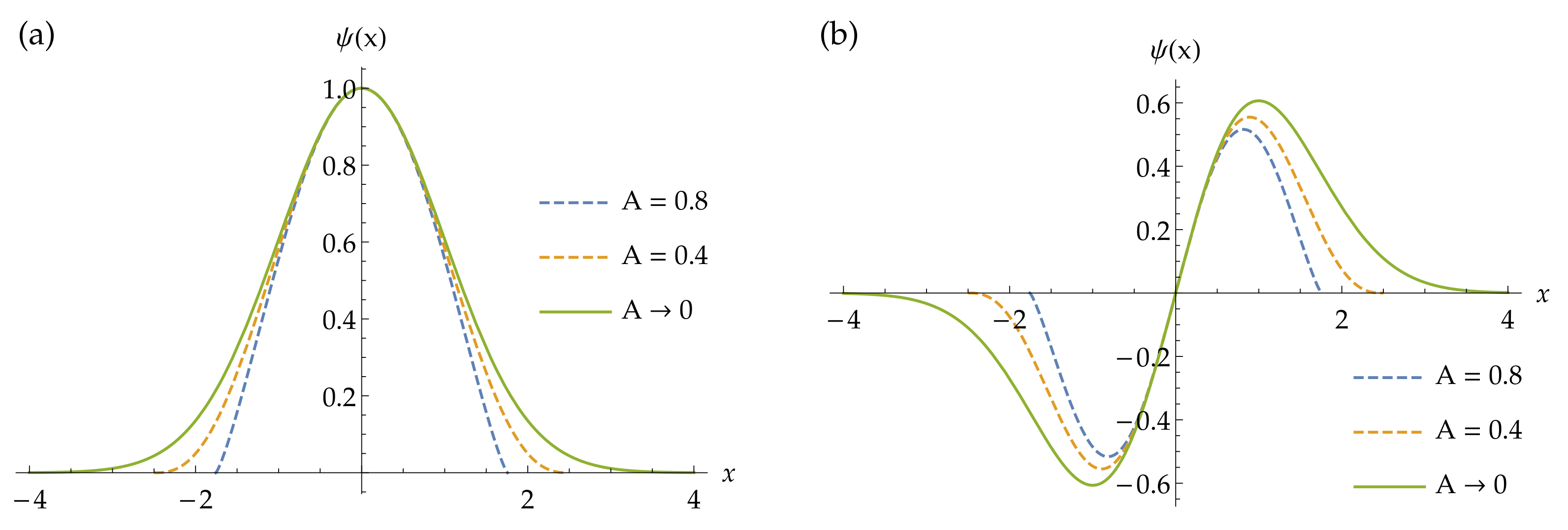
Finding the limit of the wavefunctions as A approaches zero
one acquires the Hermite polynomials multiplied by the weight function
where , and energy . One observes a change in the shape and in the domain of the wavefunctions by varying the parameter A as shown in Figure 1.
4.3. Coulomb Potential
The last example of well-known potentials presented in this section is the Coulomb potential.
By choosing , , and changing the sign of the parameter , one obtains from Equations (26) and (27) the first two wavefunctions:
As a consequence of the choice of , the cosine function shifts to the sine function. Moreover, like in the above example, in denominator of the function the constant of integration is attached, now equal . The corresponding energy is
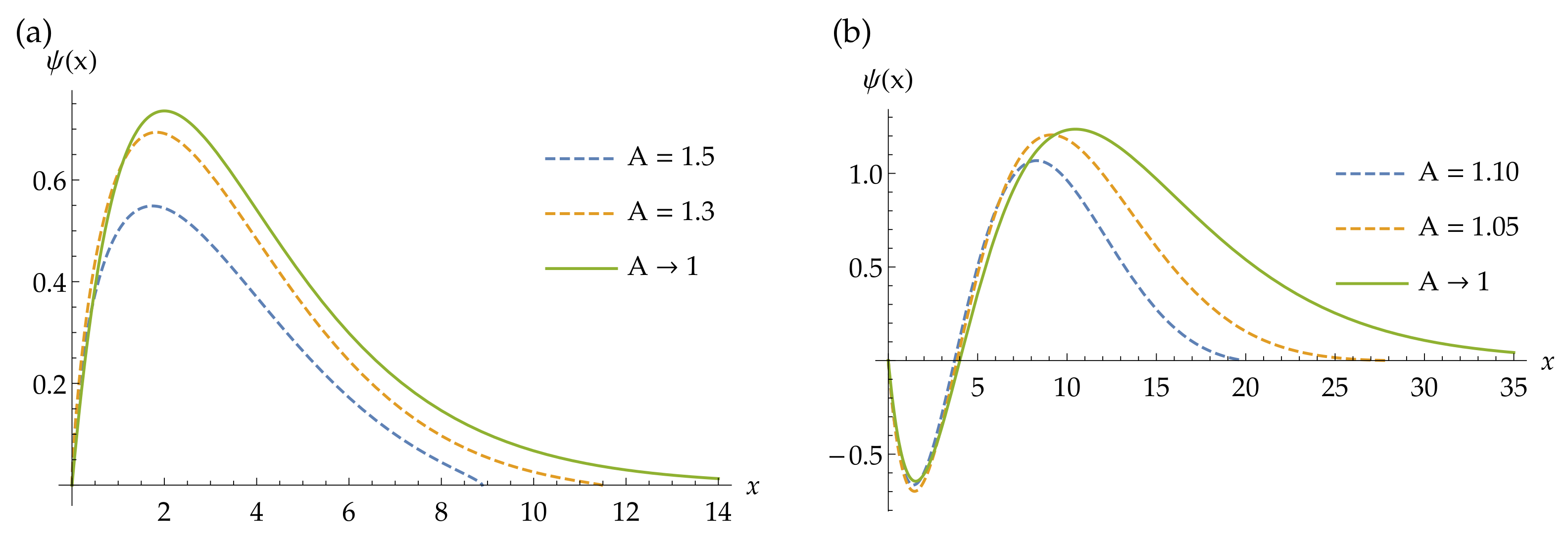
By applying the same reasoning as in the previous case, one arrives at the reformulation of the wavefunctions and the energy as A approaches unity.
Finding the limit of the wavefunctions, one obtains the generalized Laguerre polynomials multiplied by the weight function
noting that , , and energy .
As in the previous example, by varying the parameter A, one observes that wavefunctions given by Equation (39) tend to the standard solutions of the Coulomb potential, see Figure 2.
The above examples do not exhaust all possibilities of the exact solutions to the Schrödinger equation obtainable by this procedure, which also encompass the Morse potential. The presentation of the solutions to these potentials is aimed at convincing the reader of the comprehensiveness and usefulness of this method. Subsequent section is devoted to discussion of the applicability of the method.
5. Applications
The calculations for the potentials examined in the previous section prove that the method can successfully determine the ground state and the excited bound states from a new perspective. The solution to the hyperbolic potentials, such as the Morse potential, can also be recovered by the presented technique. Furthermore, the method can be generalized by extending the starting Equation (2) from the Ricatti equation to a different type [27],
Instead of a quadratic function, the right-hand side admits a rational function in , with the lower index denoting the degree of the corresponding polynomial.
Finally, applying the Equation (42) for with fixed parameters, one obtains a new exactly solvable potential of the inverse square root,
The form of the ground state is particularly simple,
while the excited states are also expressible by analytic terms [27]. Similar calculations, albeit more tedious, can be carried out to arrive at a more general version of the inverse square root potential. Moreover, by extending the order of the polynomial, , it is possible to acquire exactly solvable potentials consisting of inverse of the higher degree roots.
Thus, the Ricatti equation studied in the present paper can be thought of as one of the simplest examples of starting equations for a more general procedure. Hopefully, future research will shed light on the subject of exact solutions of the Schrödinger equation.
However, hitherto used starting Equations (2) and (42) do not allow to achieve the Airy functions for the constant force field, . Not much is known about the applicability of the presented method for continuous spectrum. It would be interesting to explore other limitations of the method since this would put bounds on any technique using shape-invariance.
On the other hand, 3D potentials with the shape-invariance property are known [12]. Therefore, one is tempted to believe that the method considered in this paper shall also have extension to the three dimensional case. To this end, one can employ separation of variables, widely used to solve the Schrödinger equation. As an example, in the case of 3D Coulomb potential with spherical symmetry the radial part satisfies the shape-invariance condition. Thus, the function admits continued fraction form.
The possible applications of the method and its results extend to the domain of numerical calculations as analytical basis functions [29]. One of the most widely used technique to solve differential equations is the finite element method of B-spline type, applied with great success in numerical atomic calculations [30,31]. Newly found functions might be convenient for generating bases used in finite element technique.
6. Concluding Remarks
For many years, a lot of efforts have been devoted to solving the Schrödinger equation for various potentials. In this contribution, the general form of the potential given by Equation (29) was found and solved. It is stressed that there is only one form of the potential, which means that all special cases (the harmonic oscillator potential, the Coulomb potential, and others) are obtained by an appropriate choice of parameters.
The results presented in this contribution are a continuation and generalization of the previous work [27]. In this earlier paper, the expressions for the coefficients , , and were not presented in the general form. The improvement, shown in the present article, enables one to derive the general form of the family of potentials that are exactly solvable using the described method. One of the most interesting contributions of this paper is the derivation of explicit Equation (16) for in the case of excited states, , as the consequence of the particular symmetry of the Ricatti equation.
Finally, it is worth noting that the formalism can be generalized to achieve the new exactly solvable potentials by another choice of the equation involving . The present contribution can be modified by choosing a rational function instead of the quadratic one, following similar steps as in [27]. It is conjecture that every potential that admits solutions to the Schrödinger equation expressible via orthogonal polynomials can be obtained by this method. Furthermore, there are several possible extensions that might lead to exactly solvable potentials yet unknown.
Funding
This research received no external funding.
Conflicts of Interest
The authors declare no conflict of interest.
References
- Sommerfeld, A. Atombau und Spektrallinien; Friedrich Vieweg und Sohn: Braunschweig, Germany, 1919. [Google Scholar]
- Konishi, K.; Paffuti, G. Quantum Mechanics. A New Introduction; Oxford University Press: New York, NY, USA, 2009. [Google Scholar]
- Dereziński, J.; Wrochna, M. Exactly Solvable Schrödinger Operators. Ann. Henri Poincare 2011, 12, 397–418. [Google Scholar] [CrossRef] [Green Version]
- Infeld, L.; Hull, T.E. The factorization method. Rev. Mod. Phys. 1951, 23, 21–68. [Google Scholar] [CrossRef]
- Sukumar, C.V. Supersymmetry, factorization of the Schrödinger equation and a Hamiltonian hierarchy. J. Phys. Math. Gen. 1985, 18, L57. [Google Scholar] [CrossRef]
- Dong, S.H. Factorization Method in Quantum Mechanics; Springer: Dordrecht, The Netherlands, 2007. [Google Scholar]
- Bagchi, B.K. Supersymmetry in Quantum and Classical Mechanics; Taylor & Francis Ltd.: London, UK, 2019. [Google Scholar]
- David, J.; Fernandez, C. Supersymmetric Quantum Mechanics. AIP Conf. Proc. 2010, 1287, 3–36. [Google Scholar]
- Gendenshtein, L. Derivation of exact spectra of the Schrödinger equation by means of supersymmetry. JETP Lett. 1983, 38, 356–359. [Google Scholar]
- Chuan, C. Exactly solvable potentials and the concept of shape invariance. J. Phys. A Math. Gen. 1991, 24, L1165–L1174. [Google Scholar] [CrossRef]
- Bougie, J.; Gangopadhyaya, A.; Mallow, J.V.; Rasinariu, C. Supersymmetric quantum mechanics and solvable models. Symmetry 2012, 4, 452–473. [Google Scholar] [CrossRef] [Green Version]
- Cooper, F.; Khare, A.; Sukhatme, U. Supersymmetry and quantum mechanics. Phys. Rep. 1995, 251, 267–385. [Google Scholar] [CrossRef] [Green Version]
- Dabrowska, J.W.; Khare, A.; Sukhatme, U.P. Explicit Wavefunctions for Shape-Invariant Potentials by Operator Techniques. J. Phys. A Math. Gen. 1988, 21, L195–L200. [Google Scholar] [CrossRef]
- Levai, G. A search for shape-invariant solvable potentials. J. Phys. A Math. Gen. 1989, 22, 689–702. [Google Scholar] [CrossRef]
- Bougie, J.; Gangopadhyaya, A.; Mallow, J.V.; Rasinariu, C. Generation of a novel exactly solvable potential. Phys. Lett. A 2015, 379, 2180–2183. [Google Scholar] [CrossRef] [Green Version]
- Benbourenane, J.; Eleuch, H. Exactly Solvable New Classes of Potentials with Finite Discrete Energies. Results Phys. 2020, 17, 103034. [Google Scholar] [CrossRef]
- Barclay, D.T.; Maxwell, C.J. Shape invariance and the SWKB series. Phys. Lett. A 1991, 157, 357–360. [Google Scholar] [CrossRef]
- Eleuch, H.; Hilke, M. ERS approximation for solving Schrödinger’s equation and applications. Results Phys. 2018, 11, 1044–1047. [Google Scholar] [CrossRef]
- Odake, S.; Sasaki, R. Another set of infinitely many exceptional (x‘) Laguerre polynomials. Phys. Lett. B 2010, 684, 173–176. [Google Scholar] [CrossRef] [Green Version]
- Bagrov, V.; Gitman, D. Exact Solutions of Relativistic Wave Equations; Kluwer Academic Publishers: Dordrecht, The Netherlands, 1990. [Google Scholar]
- Eleuch, H.; Rustovtsev, Y.V.; Scully, M. New analytic solution of Schrödinger’s equation. Europhys. Lett. 2010, 89, 50004. [Google Scholar] [CrossRef]
- Miller, S.C. Continued-fraction solutions of the one-dimensional Schrödinger equation. Phys. Rev. D 1975, 12, 3838. [Google Scholar] [CrossRef]
- Jones, W.B.; Thron, W.J. Continued Fractions: Analytic Theory and Applications; Addison-Wesley Publishing Company: Reading, PA, USA, 1980. [Google Scholar]
- Haley, S. An underrated entanglement: Riccati and Schrödinger equations. Am. J. Phys. 1997, 3, 237. [Google Scholar] [CrossRef]
- Rajchel, K. The shape invariance condition. Concepts Phys. 2006, 3, 25–32. [Google Scholar]
- Grandati, Y.; Berard, A. Rational solutions for the Riccati–Schrödinger equations associated to translationally shape invariant potentials. Ann. Phys. 2010, 325, 1235–1259. [Google Scholar] [CrossRef] [Green Version]
- Rajchel, K. New Solvable Potentials with Bound State Spectrum. Acta Phys. Pol. B 2017, 48, 757–764. [Google Scholar] [CrossRef] [Green Version]
- Reid, W.T. Ricatti Differential Equations; Academic Press: New York, NY, USA; London, UK, 1972. [Google Scholar]
- Vilkas, M.J.; Ishikawa, Y.; Koc, K. Quadratically convergent multiconfiguration Dirac-Fock and multireference relativistic configuration-interaction calculations for many-electron systems. Phys. Rev. E 1998, 58, 5096. [Google Scholar] [CrossRef]
- Desclaux, J.P.; Dolbeault, J.; Esteban, M.J.; Indelicato, P.; Sere, E. Computational Approaches of Relativistic Models in Quantum Chemistry; Elsevier: Amsterdam, The Netherlands, 2003; pp. 453–483. [Google Scholar]
- De Boor, C. A Practical Guide to Splines; Springer: New York, NY, USA, 1978. [Google Scholar]
Figure 1.
The solutions of the Schrödinger equation with potential given by Equation (29) for certain values of parameter A (dotted lines). The wavefunctions: the ground state (a) and the first excited state (b) both approach the solutions to the harmonic oscillator potential (solid lines) as .
Figure 1.
The solutions of the Schrödinger equation with potential given by Equation (29) for certain values of parameter A (dotted lines). The wavefunctions: the ground state (a) and the first excited state (b) both approach the solutions to the harmonic oscillator potential (solid lines) as .

Figure 2.
The solutions of the Schrödinger equation with potential given by Equation (29) for certain values of parameter A (dotted lines), while the parameter . The wavefunctions: the ground state (a) and the first excited state (b) both approach the solutions to the Coulomb potential (solid lines) as .

Publisher’s Note: MDPI stays neutral with regard to jurisdictional claims in published maps and institutional affiliations. |
© 2021 by the author. Licensee MDPI, Basel, Switzerland. This article is an open access article distributed under the terms and conditions of the Creative Commons Attribution (CC BY) license (https://creativecommons.org/licenses/by/4.0/).
Share and Cite
MDPI and ACS Style
Rajchel, K. A New Constructive Method for Solving the Schrödinger Equation. Symmetry 2021, 13, 1879. https://doi.org/10.3390/sym13101879
AMA Style
Rajchel K. A New Constructive Method for Solving the Schrödinger Equation. Symmetry. 2021; 13(10):1879. https://doi.org/10.3390/sym13101879
Chicago/Turabian StyleRajchel, Kazimierz. 2021. "A New Constructive Method for Solving the Schrödinger Equation" Symmetry 13, no. 10: 1879. https://doi.org/10.3390/sym13101879
Note that from the first issue of 2016, this journal uses article numbers instead of page numbers. See further details here.