
A Generalized Strain Energy-Based Homogenization Method for 2-D and 3-D Cellular Materials with and without Periodicity Constraints †


Abstract
:1. Introduction
2. Generalized Strain Energy-Based Homogenization Method
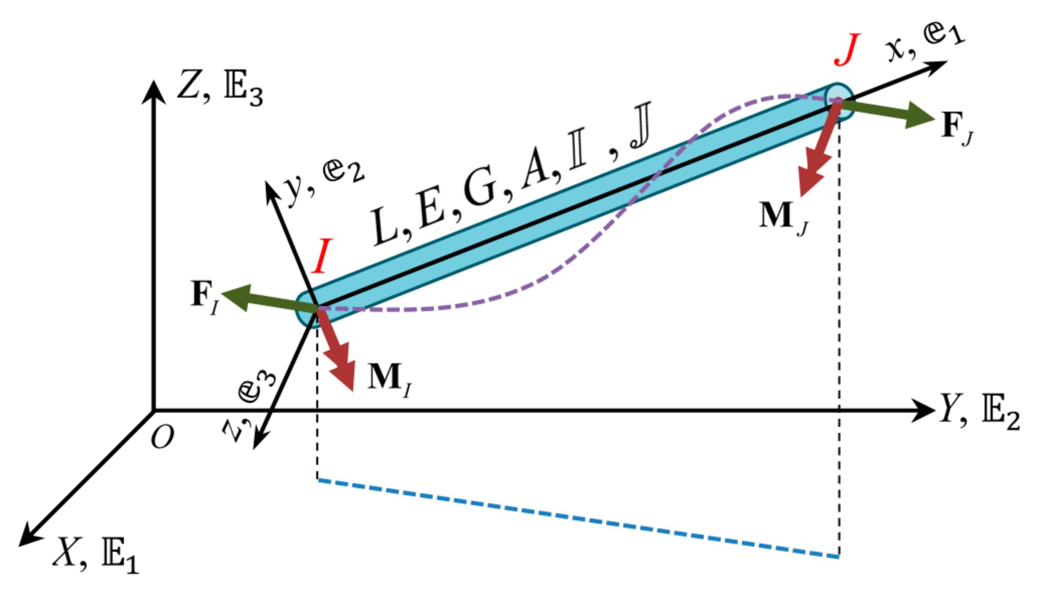
2.1. Matrix Method for Spatial Frames
2.2. Hill’s Lemma
2.3. Generalized Homogenization Method
2.4. Extension to Periodic Materials
3. Case Studies
3.1. 2-D Cases
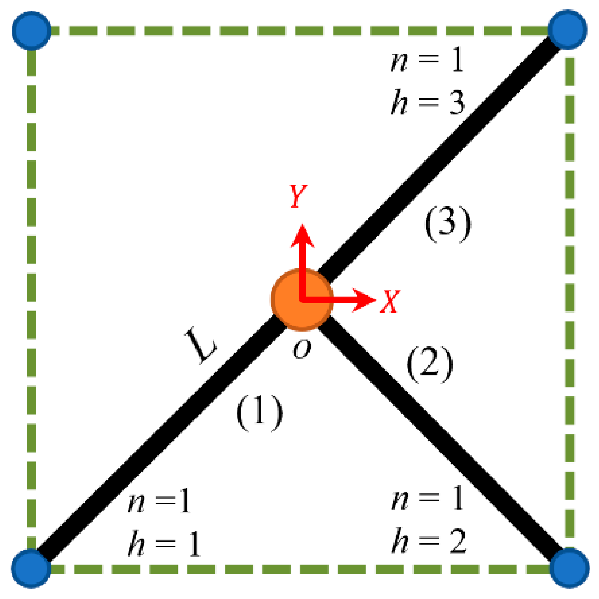
3.1.1. 2-D Homogenization without Periodicity Constraints
3.1.2. 2-D Homogenization with Periodicity Constraints
3.2. 3-D Cases
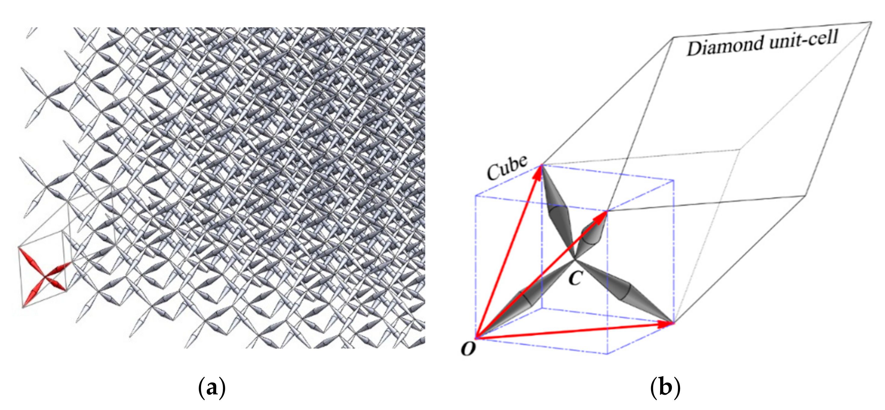
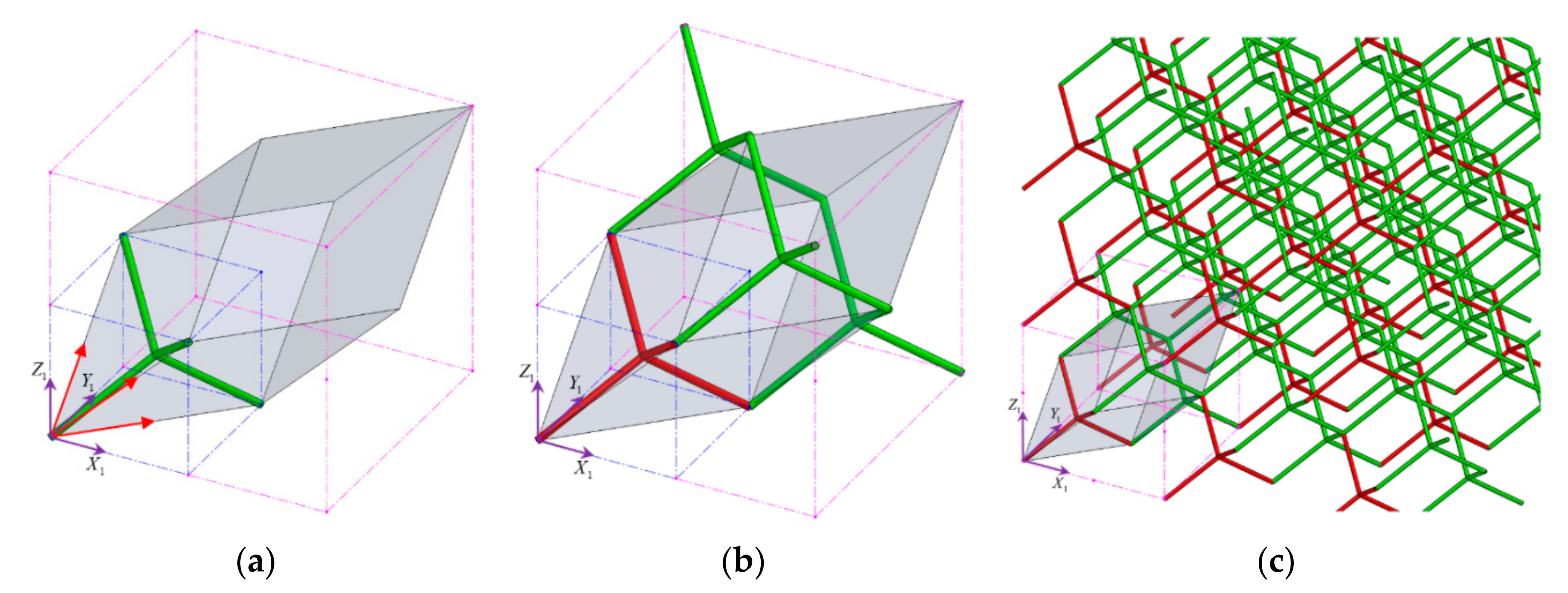
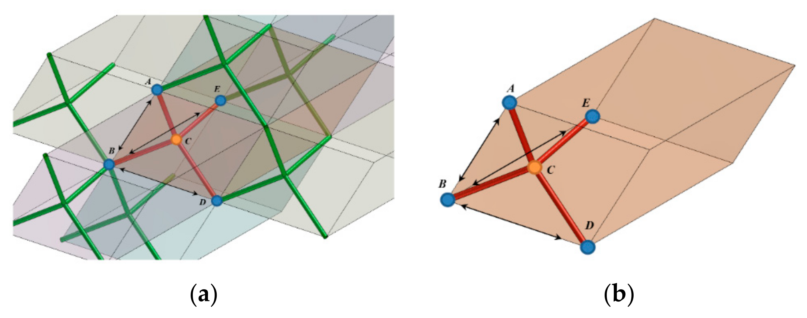
3.2.1. Pentamode Metamaterial
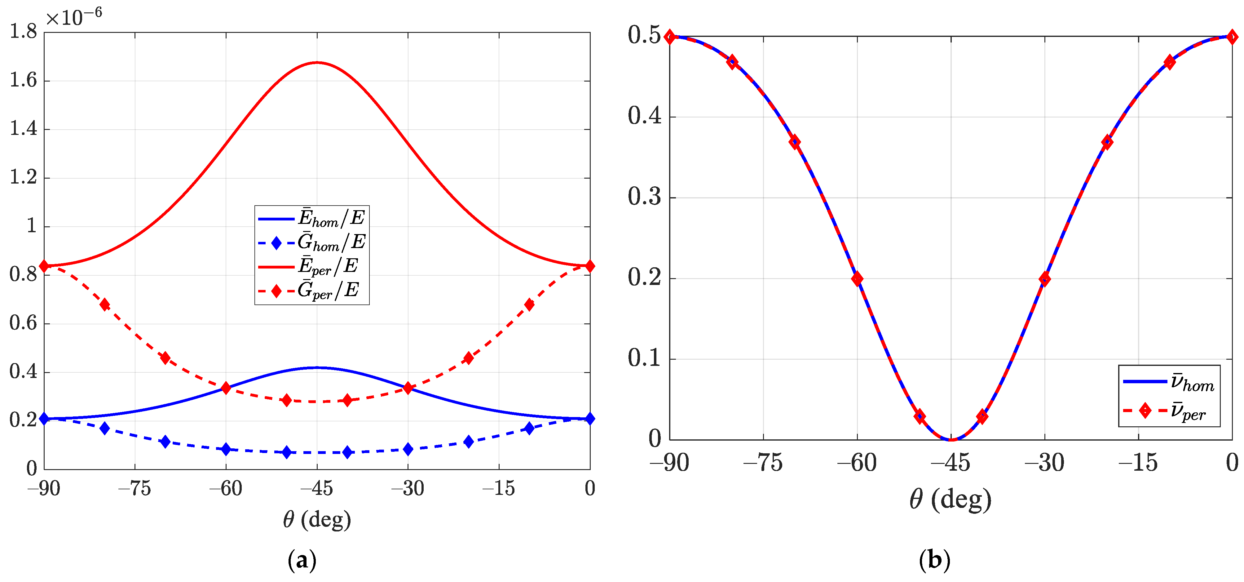
3.2.2. Homogenization without Periodicity Constraints
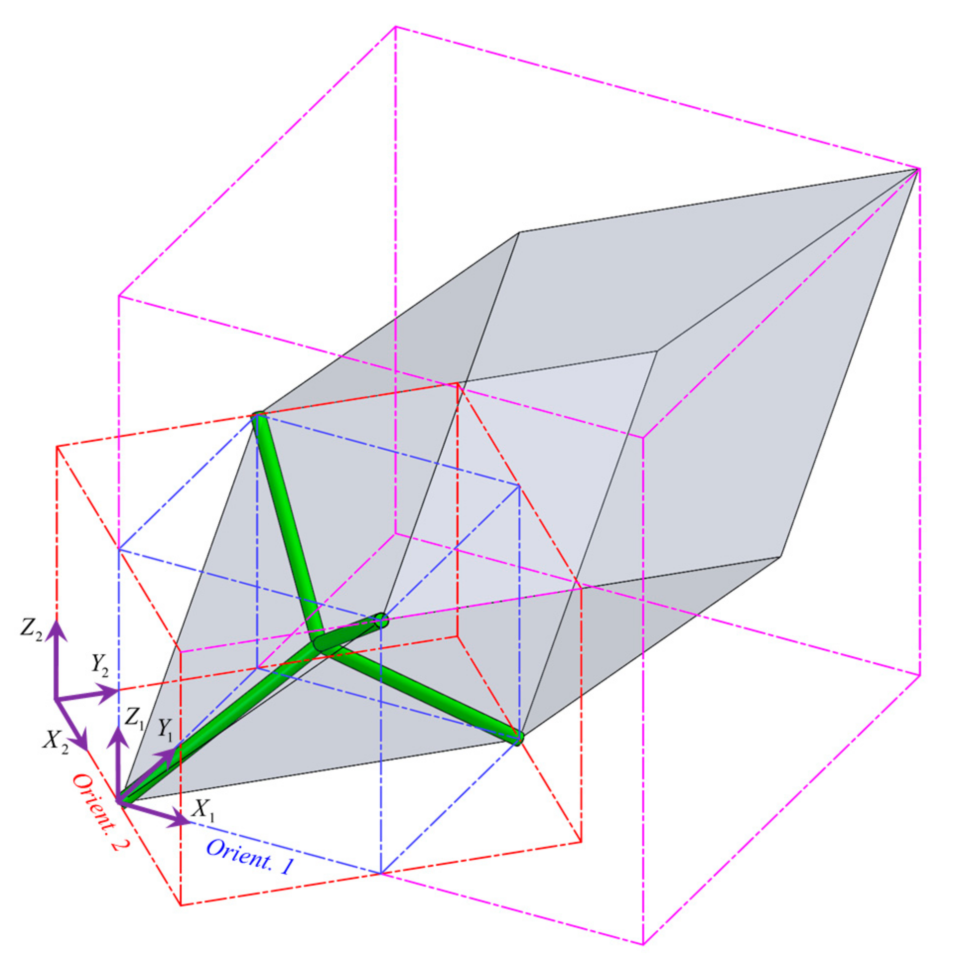
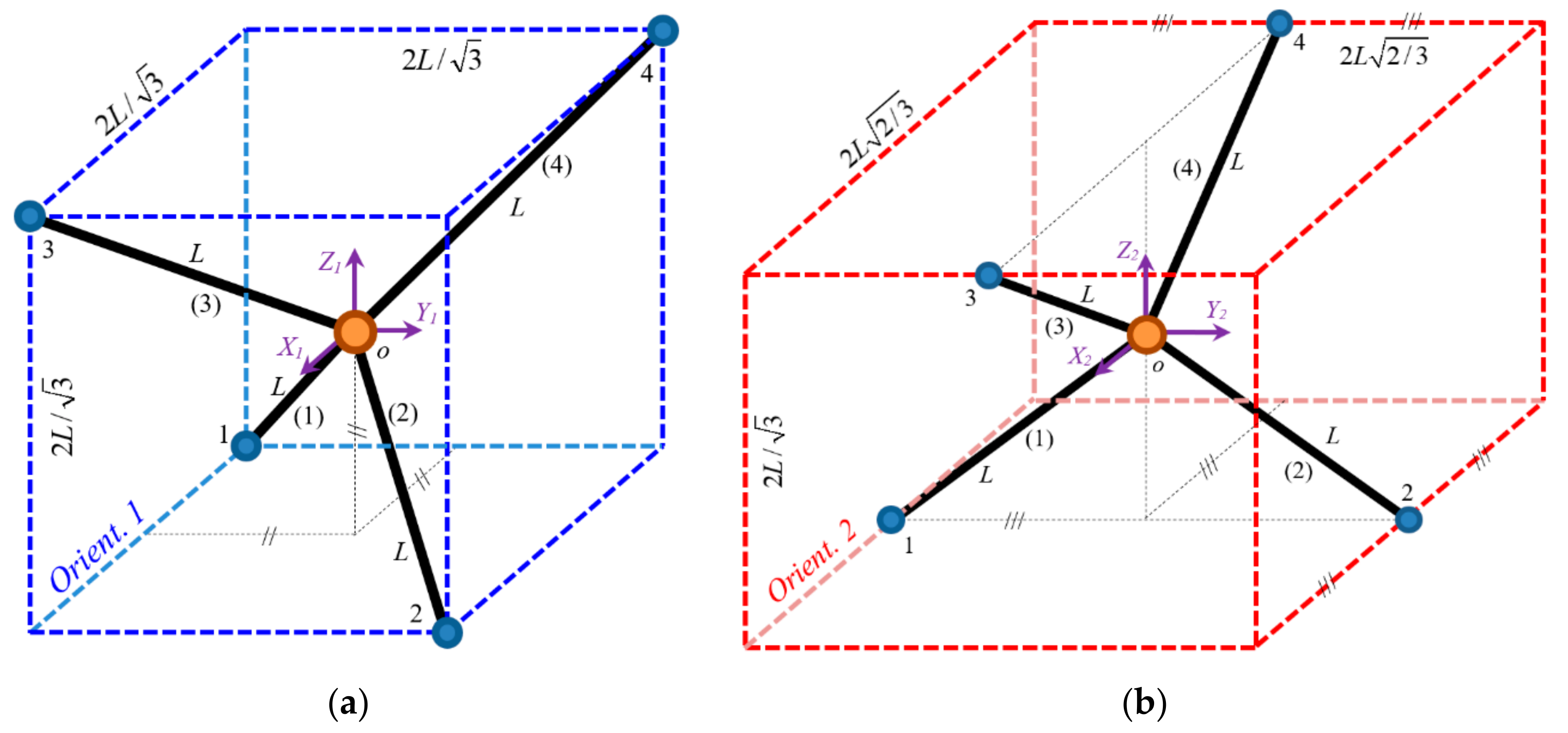
Homogenization Based on the First Representative Cell
Homogenization Based on the Second Representative Cell
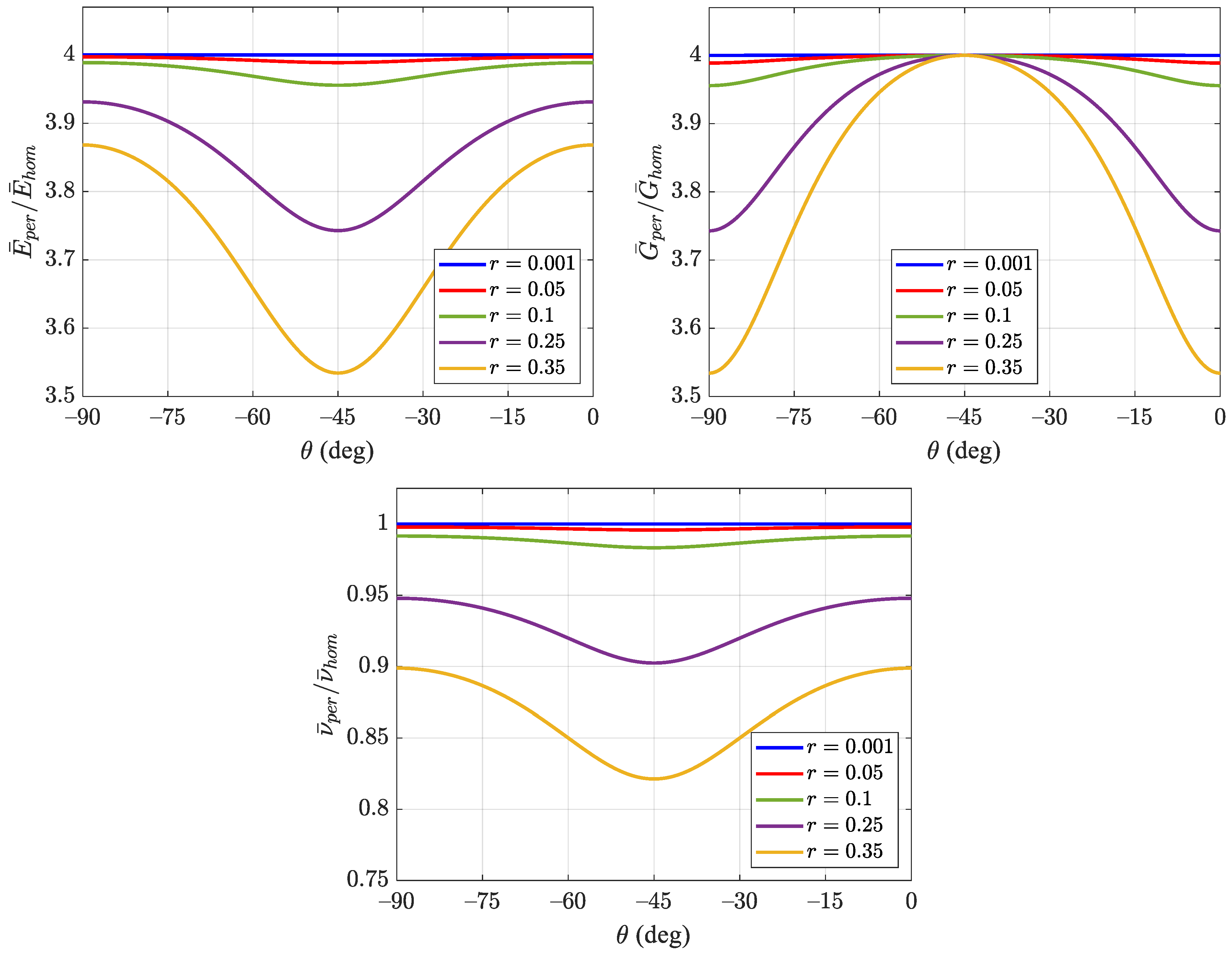
3.2.3. Homogenization with Periodicity Constraints
Homogenization Based on the First Representative Cell with Periodicity Constraints
Homogenization Based on the Second Representative Cell with Periodicity Constraints
4. Conclusions
Author Contributions
Funding
Institutional Review Board Statement
Informed Consent Statement
Acknowledgments
Conflicts of Interest
References
- Hassani, B.; Hinton, E. A review of homogenization and topology optimization I—homogenization theory for media with periodic structure. Comput. Struct. 1998, 69, 707–717. [Google Scholar] [CrossRef]
- Arabnejad, S.; Pasini, D. Mechanical properties of lattice materials via asymptotic homogenization and comparison with alternative homogenization methods. Int. J. Mech. Sci. 2013, 77, 249–262. [Google Scholar] [CrossRef] [Green Version]
- Bacigalupo, A.; Gambarotta, L. Homogenization of periodic hexa- and tetrachiral cellular solids. Compos. Struct. 2014, 116, 461–476. [Google Scholar] [CrossRef] [Green Version]
- Iltchev, A.; Marcadon, V.; Kruch, S.; Forest, S. Computational homogenisation of periodic cellular materials: Application to structural modelling. Int. J. Mech. Sci. 2015, 93, 240–255. [Google Scholar] [CrossRef]
- Lim, T.C. Auxetic Materials and Structures; Springer: Singapore, 2015. [Google Scholar]
- Ai, L.; Gao, X.-L. Three-dimensional metamaterials with a negative Poisson’s ratio and a non-positive coefficient of thermal expansion. Int. J. Mech. Sci. 2018, 135, 101–113. [Google Scholar] [CrossRef]
- Ongaro, F. Estimation of the effective properties of two-dimensional cellular materials: A review. Theor. Appl. Mech. Lett. 2018, 8, 209–230. [Google Scholar] [CrossRef]
- Xu, H.; Farag, A.; Pasini, D. Routes to program thermal expansion in three-dimensional lattice metamaterials built from tetrahedral building blocks. J. Mech. Phys. Solids 2018, 117, 54–87. [Google Scholar] [CrossRef] [Green Version]
- Lim, T.-C. Mechanics of Metamaterials with Negative Parameters; Springer Nature: Singapore, 2020. [Google Scholar]
- Lim, T.-C. An Auxetic system based on interconnected Y-elements inspired by Islamic geometric patterns. Symmetry 2021, 13, 865. [Google Scholar] [CrossRef]
- Gad, A.; Gao, X.-L.; Li, K. A strain energy-based homogenization method for 2-D and 3-D cellular materials using the micropolar elasticity theory. Compos. Struct. 2021, 265, 113594. [Google Scholar] [CrossRef]
- Warren, W.E.; Kraynik, A.M. Linear elastic behavior of a low-density Kelvin foam with open cells. J. Appl. Mech. 1997, 64, 787–794. [Google Scholar] [CrossRef]
- Tollenaere, H.; Caillerie, D. Continuous modeling of lattice structures by homogenization. Adv. Eng. Softw. 1998, 29, 699–705. [Google Scholar] [CrossRef]
- Li, K.; Gao, X.-L.; Roy, A.K. Micromechanics model for three-dimensional open-cell foams using a tetrakaidecahedral unit cell and Castigliano’s second theorem. Compos. Sci. Technol. 2003, 63, 1769–1781. [Google Scholar] [CrossRef]
- Demiray, S.; Becker, W.; Hohe, J. Strain-energy based homogenisation of two- and three-dimensional hyperelastic solid foams. J. Mater. Sci. 2005, 40, 5839–5844. [Google Scholar] [CrossRef]
- Martinsson, P.G.; Babuška, I. Homogenization of materials with periodic truss or frame micro-structures. Math. Model. Methods Appl. Sci. 2007, 17, 805–832. [Google Scholar] [CrossRef]
- Freund, J.; Karakoc, A.; Sjolund, J. Computational homogenization of regular cellular material according to classical elasticity. Mech. Mater. 2014, 78, 56–65. [Google Scholar] [CrossRef]
- Norris, A.N. Mechanics of elastic networks. Proc. R. Soc. A 2014, 470, 20140522. [Google Scholar] [CrossRef] [Green Version]
- Ongaro, F.; Barbieri, E.; Pugno, N. Mechanics of mutable hierarchical composite cellular materials. Mech. Mater. 2018, 124, 80–99. [Google Scholar] [CrossRef]
- Ai, L.; Gao, X.-L. An analytical model for star-shaped re-entrant lattice structures with the orthotropic symmetry and negative Poisson’s ratios. Int. J. Mech. Sci. 2018, 145, 158–170. [Google Scholar] [CrossRef]
- Evans, K.E.; Alderson, A. Auxetic materials: Functional materials and structures from lateral thinking. Adv. Mater. 2000, 12, 617–628. [Google Scholar] [CrossRef]
- Lakes, R.; Wojciechowski, K.W. Negative compressibility, negative Poisson’s ratio, and stability. Phys. Status Solidi (b) 2008, 245, 545–551. [Google Scholar] [CrossRef]
- Greaves, G.N.; Greer, A.L.; Lakes, R.S.; Rouxel, T. Poisson’s ratio and modern materials. Nat. Mater. 2011, 10, 823–837. [Google Scholar] [CrossRef] [PubMed]
- Lakes, R.S. Negative-Poisson’s-ratio materials: Auxetic solids. Annu. Rev. Mater. Res. 2017, 47, 63–81. [Google Scholar] [CrossRef]
- Ai, L.; Gao, X.-L. Metamaterials with negative Poisson’s ratio and non-positive thermal expansion. Compos. Struct. 2017, 162, 70–84. [Google Scholar] [CrossRef] [Green Version]
- Ai, L.; Gao, X.-L. Micromechanical modeling of 3D printable interpenetrating phase composites with tailorable effective elastic properties including negative Poisson’s ratio. J. Micromech. Mol. Phys. 2017, 2, 1750015. [Google Scholar] [CrossRef]
- Czarnecki, S.; Łukasiak, T. Recovery of the auxetic microstructures appearing in the least compliant continuum two-dimensional bodies. Phys. Status Solidi (B) 2020, 257, 1900676. [Google Scholar] [CrossRef]
- Askar, A.; Cakmak, A. A structural model of a micropolar continuum. Int. J. Eng. Sci. 1968, 6, 583–589. [Google Scholar] [CrossRef]
- Bažant, Z.; Christensen, M. Analogy between micropolar continuum and grid frameworks under initial stress. Int. J. Solids Struct. 1972, 8, 327–346. [Google Scholar] [CrossRef] [Green Version]
- Chen, J.; Huang, Y.; Ortiz, M. Fracture analysis of cellular materials: A strain gradient model. J. Mech. Phys. Solids 1998, 46, 789–828. [Google Scholar] [CrossRef]
- Wang, X.L.; Stronge, W.J. Micropolar theory for two—Dimensional stresses in elastic honeycomb. Proc. R. Soc. A Math. Phys. Eng. Sci. 1999, 455, 2091–2116. [Google Scholar] [CrossRef]
- Kumar, R.S.; McDowell, D.L. Generalized continuum modeling of 2-D periodic cellular solids. Int. J. Solids Struct. 2004, 41, 7399–7422. [Google Scholar] [CrossRef]
- Park, S.K.; Gao, X.-L. Micromechanical modeling of honeycomb structures based on a modified couple stress theory. Mech. Adv. Mater. Struct. 2008, 15, 574–593. [Google Scholar] [CrossRef]
- Bacigalupo, A.; Gambarotta, L. Generalized micropolar continualization of 1D beam lattices. Int. J. Mech. Sci. 2019, 155, 554–570. [Google Scholar] [CrossRef] [Green Version]
- Niu, B.; Yan, J. A new micromechanical approach of micropolar continuum modeling for 2-D periodic cellular material. Acta Mech. Sin. 2016, 32, 456–468. [Google Scholar] [CrossRef]
- Weaver, W.; Gere, J.M. Matrix Analysis of Framed Structures, 3rd ed.; Springer: New York, NY, USA, 1990. [Google Scholar]
- Li, K.; Gao, X.-L.; Roy, A. Micromechanical modeling of three-dimensional open-cell foams using the matrix method for spatial frames. Compos. Part B Eng. 2005, 36, 249–262. [Google Scholar] [CrossRef]
- Hill, R. Elastic properties of reinforced solids: Some theoretical principles. J. Mech. Phys. Solids 1963, 11, 357–372. [Google Scholar] [CrossRef]
- Gao, X.-L. Extended Hill’s lemma for non-Cauchy continua based on the simplified strain gradient elasticity theory. J. Micromech. Mol. Phys. 2016, 3, 1640004. [Google Scholar] [CrossRef]
- Gad, A.I.; Gao, X.-L. Extended Hill’s lemma for non-Cauchy continua based on a modified couple stress theory. Acta Mech. 2020, 231, 977–997. [Google Scholar] [CrossRef]
- Gad, A.I.; Gao, X.-L. Two versions of the extended Hill’s lemma for non-Cauchy continua based on the couple stress theory. Math. Mech. Solids 2021, 26, 244–262. [Google Scholar] [CrossRef]
- Li, S.; Wang, G. Introduction to Micromechanics and Nanomechanics; World Scientific: Singapore, 2008. [Google Scholar]
- Liu, Q. Hill’s lemma for the average-field theory of Cosserat continuum. Acta Mech. 2013, 224, 851–866. [Google Scholar] [CrossRef]
- Warren, W.E.; Kraynik, A.M. The linear elastic properties of open-cell foams. J. Appl. Mech. 1988, 55, 341–346. [Google Scholar] [CrossRef]
- Drago, A.; Pindera, M.J. Micro-macromechanical analysis of heterogeneous materials: Macroscopically homoge-neous vs periodic microstructures. Compos. Sci. Technol. 2007, 67, 1243–1263. [Google Scholar] [CrossRef]
- Liu, Q. A new version of Hill’s lemma for Cosserat continuum. Arch. Appl. Mech. 2015, 85, 761–773. [Google Scholar] [CrossRef]
- Bilski, M.; Pigłowski, P.; Wojciechowski, K. Extreme Poisson’s ratios of honeycomb, re-entrant, and zig-zag crystals of binary hard discs. Symmetry 2021, 13, 1127. [Google Scholar] [CrossRef]
- Milton, G.W.; Cherkaev, A.V. Which elasticity tensors are realizable? J. Eng. Mater. Technol. 1995, 117, 483–493. [Google Scholar] [CrossRef]
- Hayes, M. Connexions between the moduli for anistropic elastic materials. J. Elast. 1972, 2, 135–141. [Google Scholar] [CrossRef]
- Norris, A.N. Poisson’s ratio in cubic materials. Proc. R. Soc. A 2006, 462, 3385–3405. [Google Scholar] [CrossRef]
- Ting, T.C.T. Anisotropic Elasticity—Theory and Applications; Oxford University Press: New York, NY, USA, 1996. [Google Scholar]


Publisher’s Note: MDPI stays neutral with regard to jurisdictional claims in published maps and institutional affiliations. |
© 2021 by the authors. Licensee MDPI, Basel, Switzerland. This article is an open access article distributed under the terms and conditions of the Creative Commons Attribution (CC BY) license (https://creativecommons.org/licenses/by/4.0/).
Share and Cite
Gad, A.I.; Gao, X.-L. A Generalized Strain Energy-Based Homogenization Method for 2-D and 3-D Cellular Materials with and without Periodicity Constraints. Symmetry 2021, 13, 1870. https://doi.org/10.3390/sym13101870
Gad AI, Gao X-L. A Generalized Strain Energy-Based Homogenization Method for 2-D and 3-D Cellular Materials with and without Periodicity Constraints. Symmetry. 2021; 13(10):1870. https://doi.org/10.3390/sym13101870
Chicago/Turabian StyleGad, Ahmad I., and Xin-Lin Gao. 2021. "A Generalized Strain Energy-Based Homogenization Method for 2-D and 3-D Cellular Materials with and without Periodicity Constraints" Symmetry 13, no. 10: 1870. https://doi.org/10.3390/sym13101870