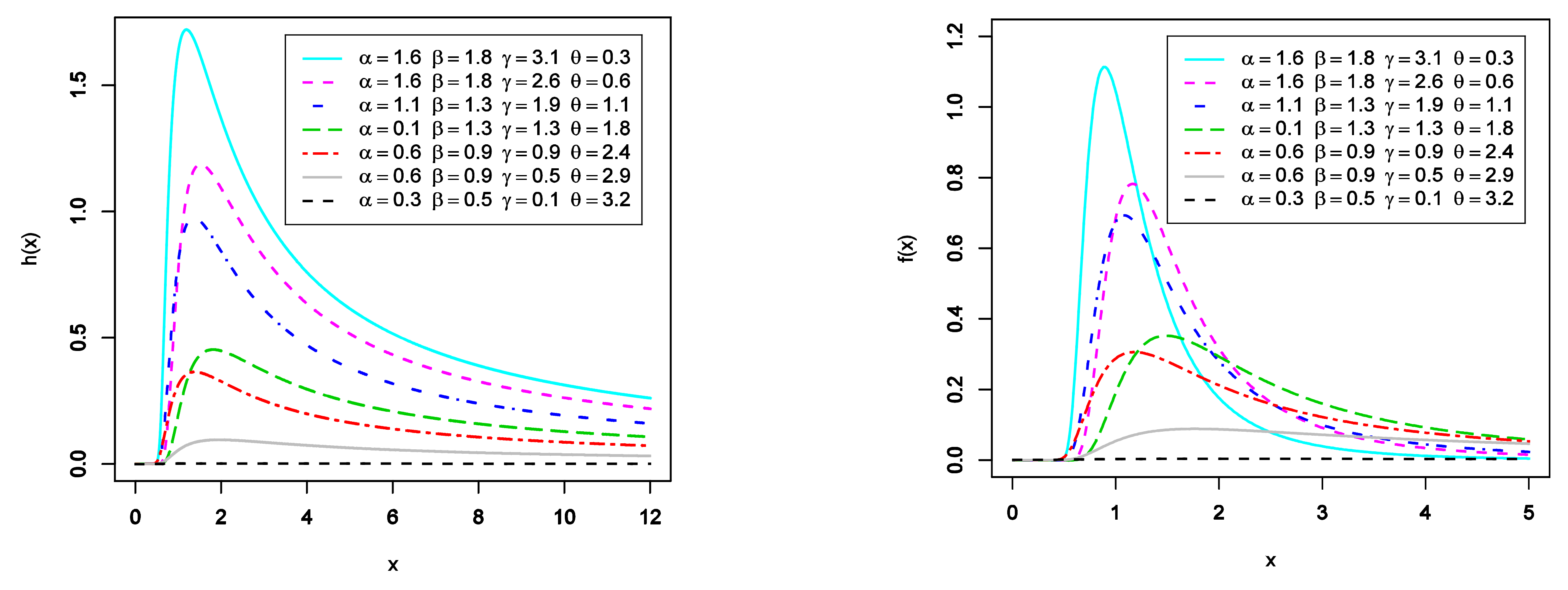
Figure 1.
The plots of HRF (left panel) and PDF (right panel) for EGIG with different choices of , , , and .
Figure 1.
The plots of HRF (left panel) and PDF (right panel) for EGIG with different choices of , , , and .
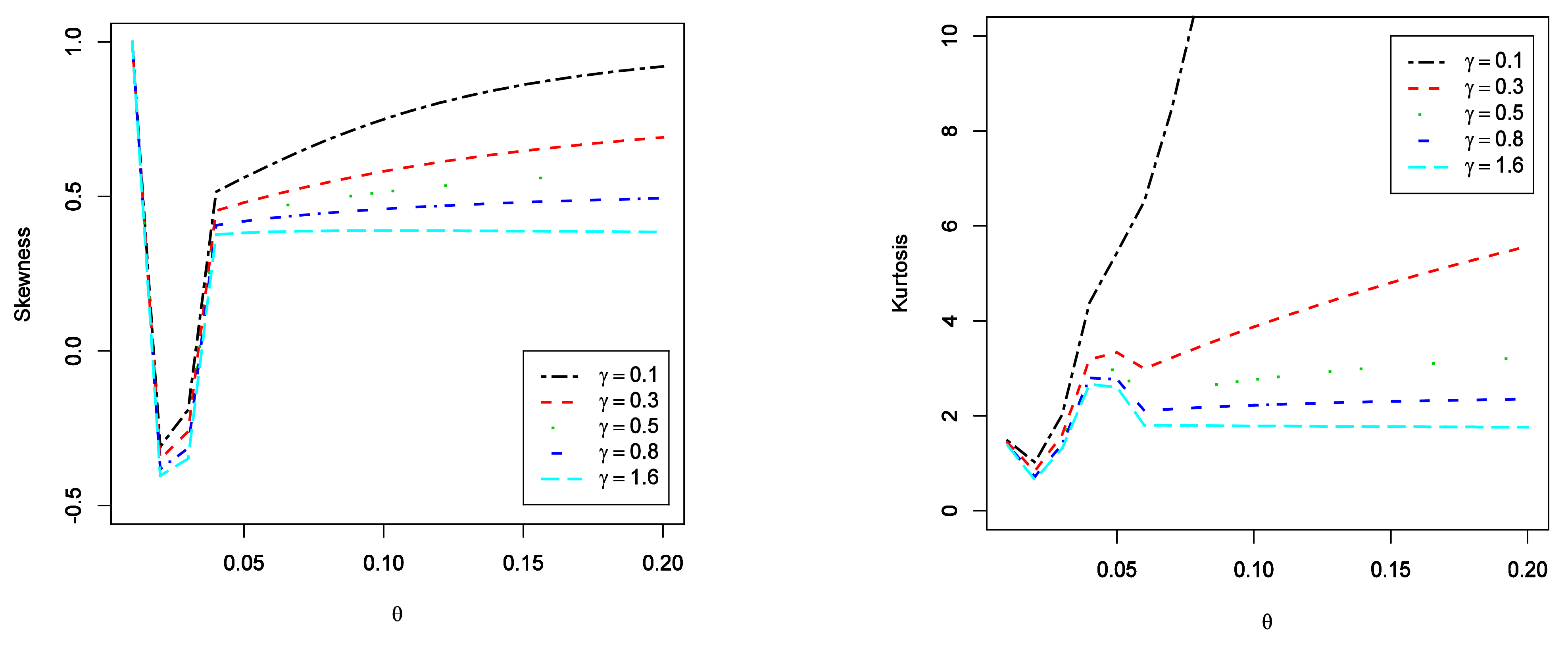
Figure 2.
The plots of (left panel) and the plots of (right panel) for the EGIG model.
Figure 2.
The plots of (left panel) and the plots of (right panel) for the EGIG model.
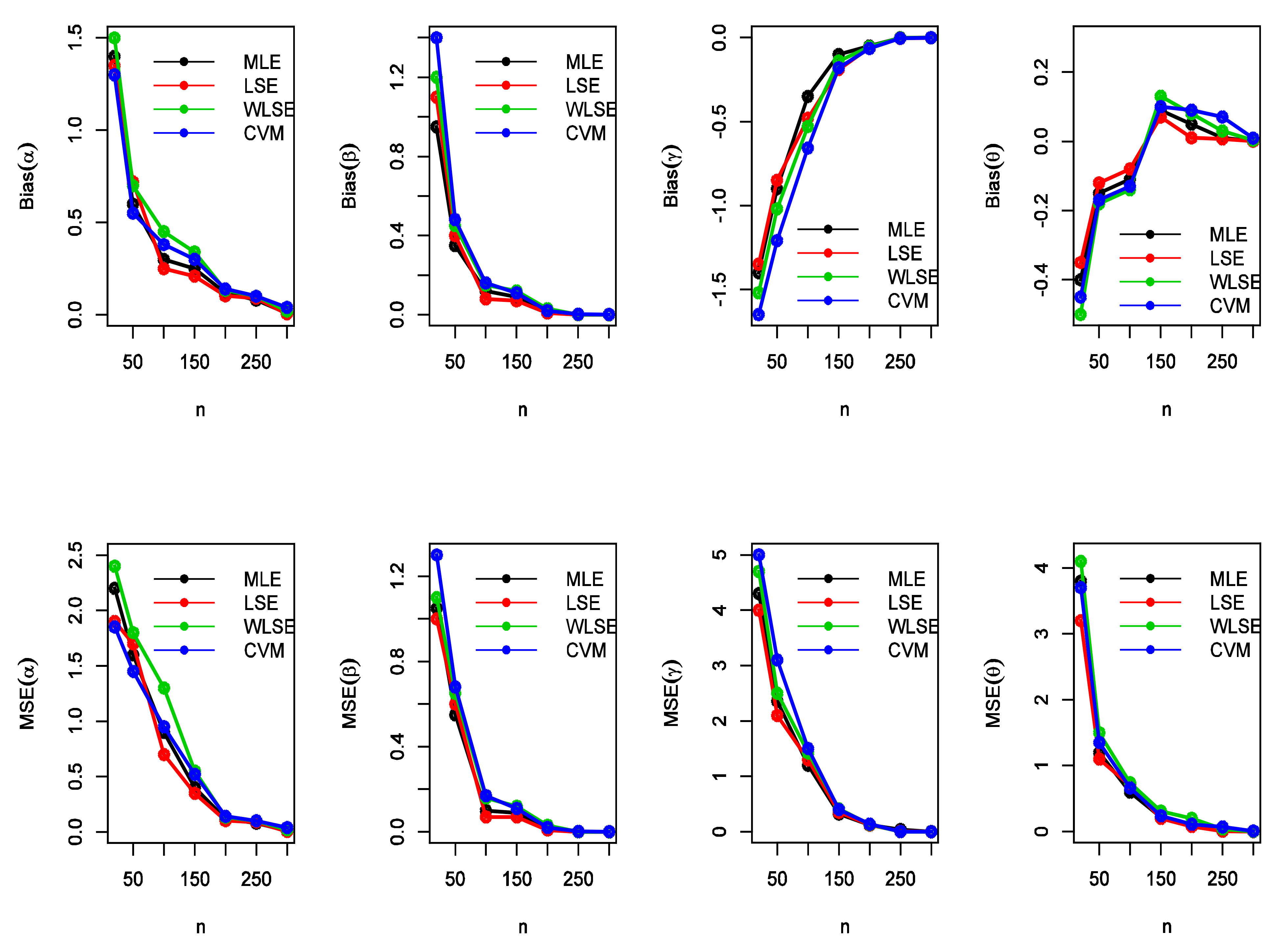
Figure 3.
The MSEs and bias estimates of the EGIG for some values of when , , ,
Figure 3.
The MSEs and bias estimates of the EGIG for some values of when , , ,
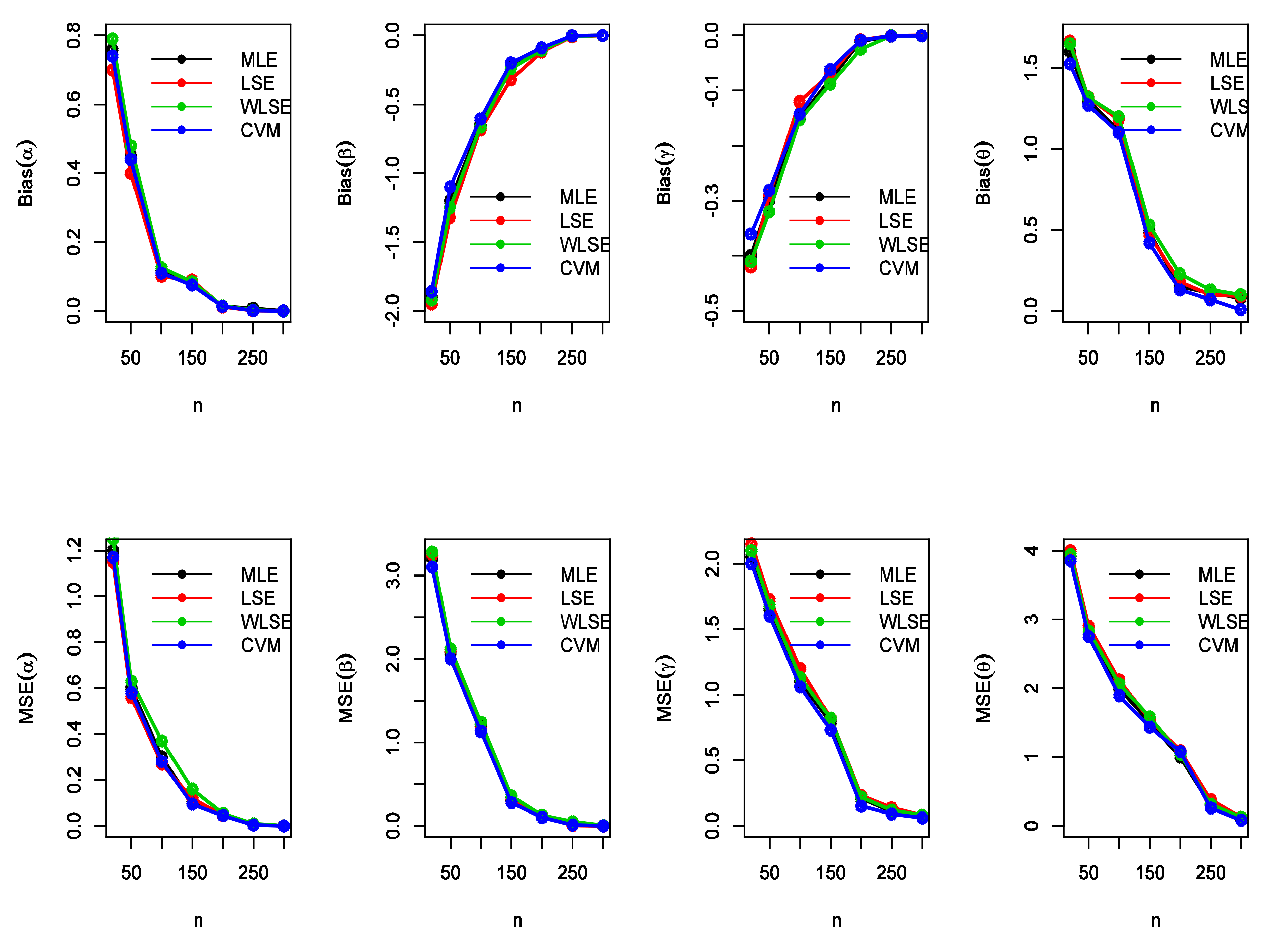
Figure 4.
The MSEs and bias estimates of the EGIG for some values of when , , ,
Figure 4.
The MSEs and bias estimates of the EGIG for some values of when , , ,
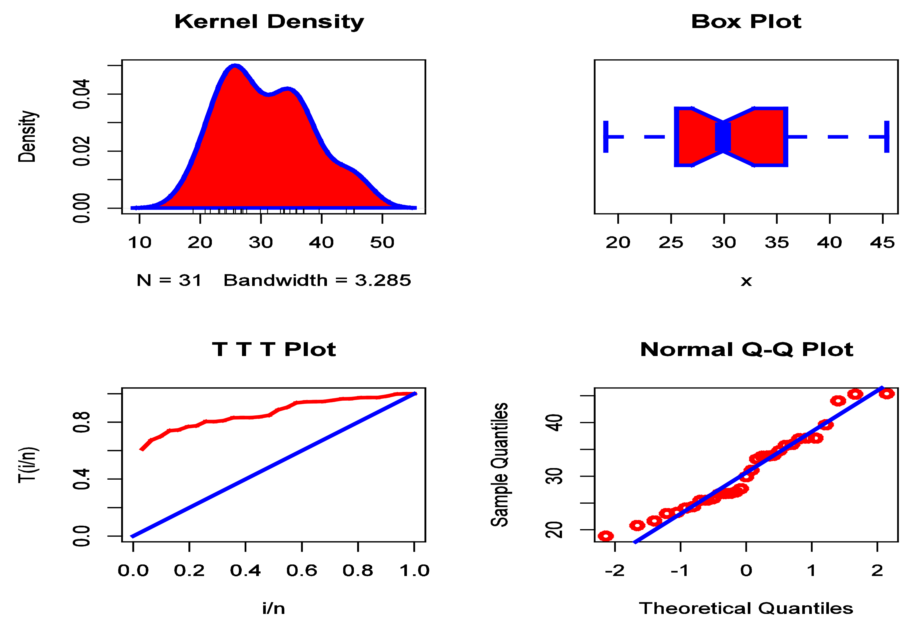
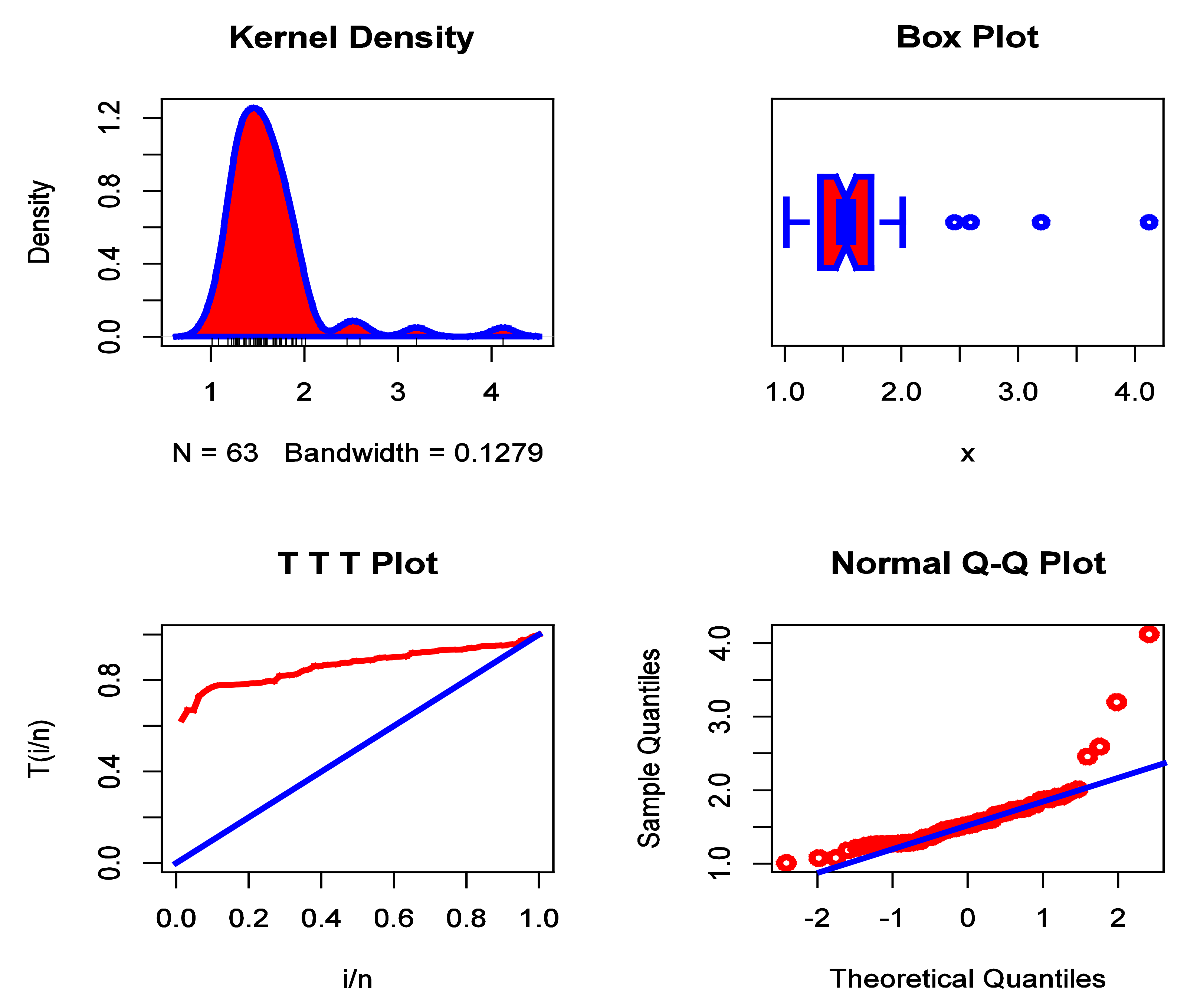
Figure 5.
The KDE plot, box plot, TTT plot, and Q–Q plot for the data set I.
Figure 5.
The KDE plot, box plot, TTT plot, and Q–Q plot for the data set I.
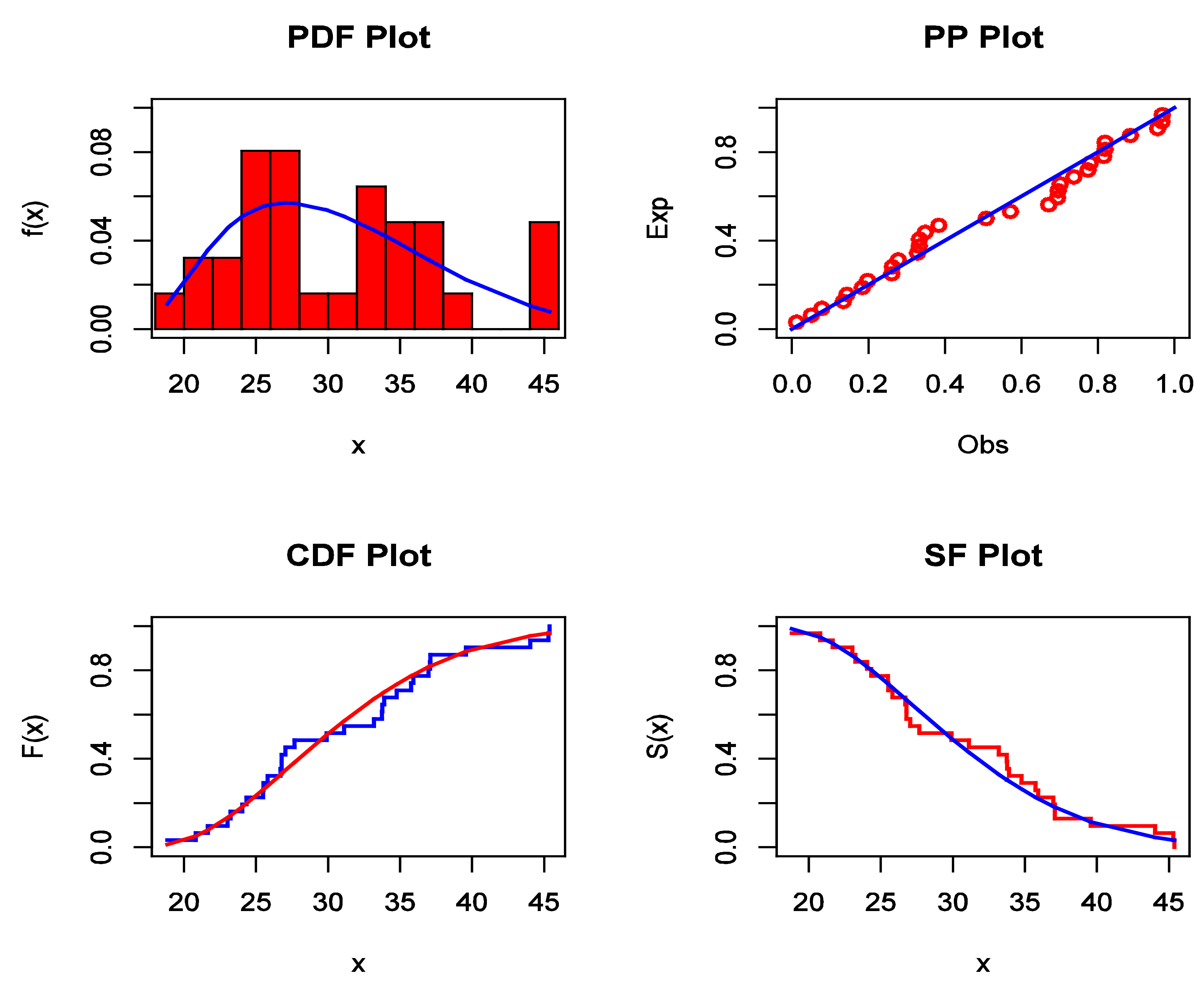
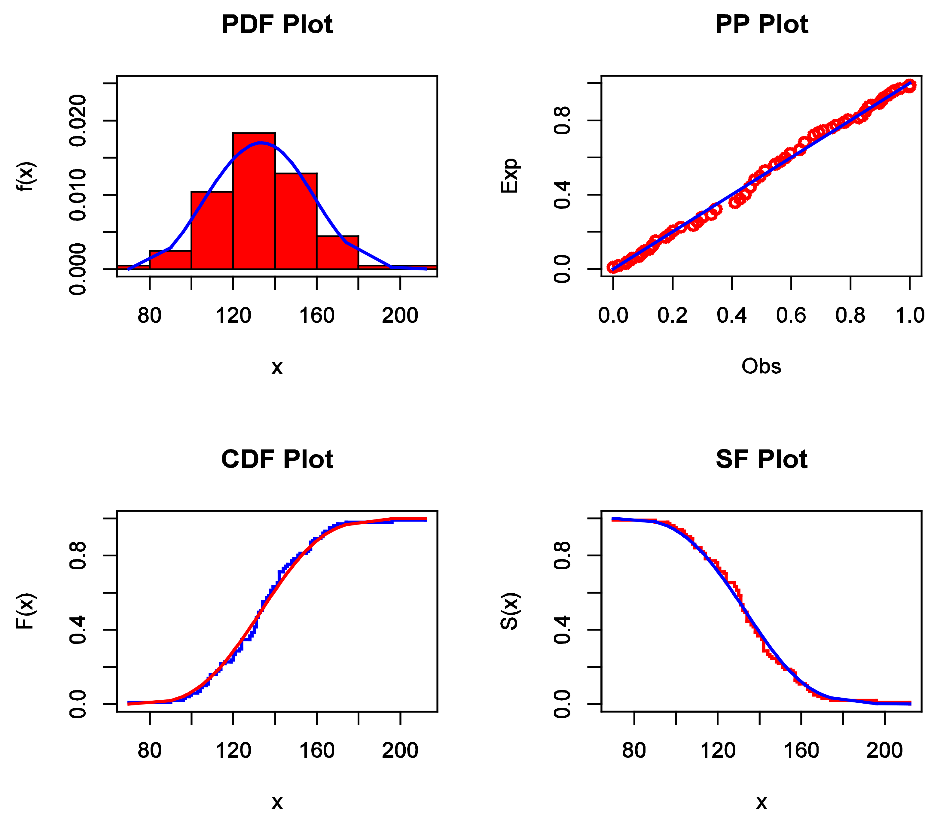
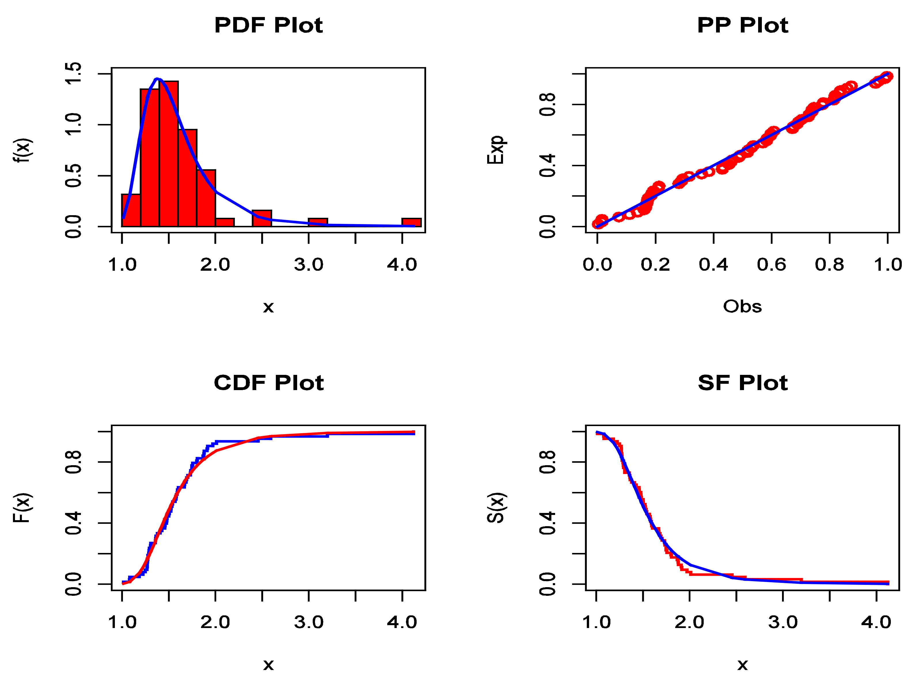
Figure 6.
The estimated PDF, P–P plot, estimated CDF, and estimated SF for data set I.
Figure 6.
The estimated PDF, P–P plot, estimated CDF, and estimated SF for data set I.
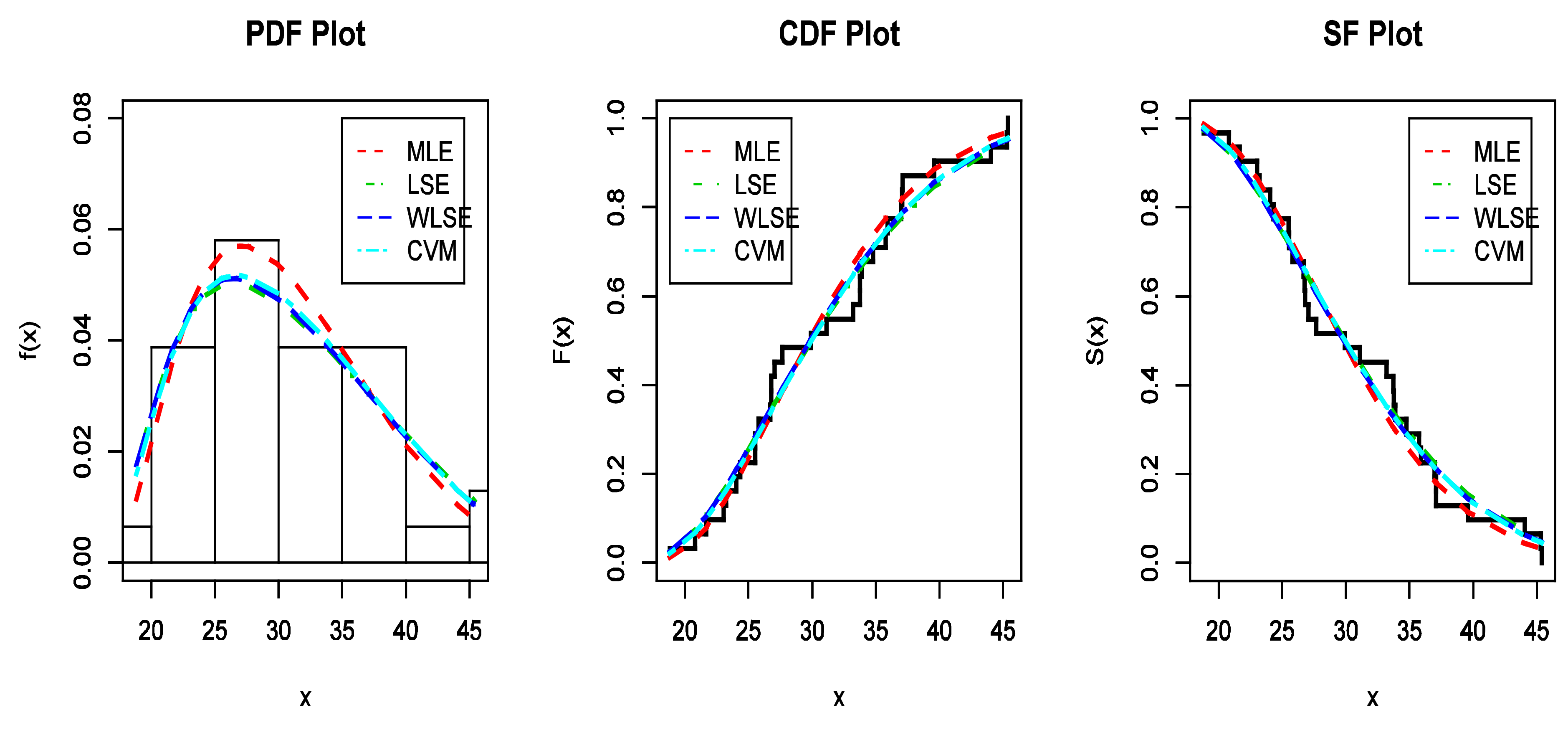
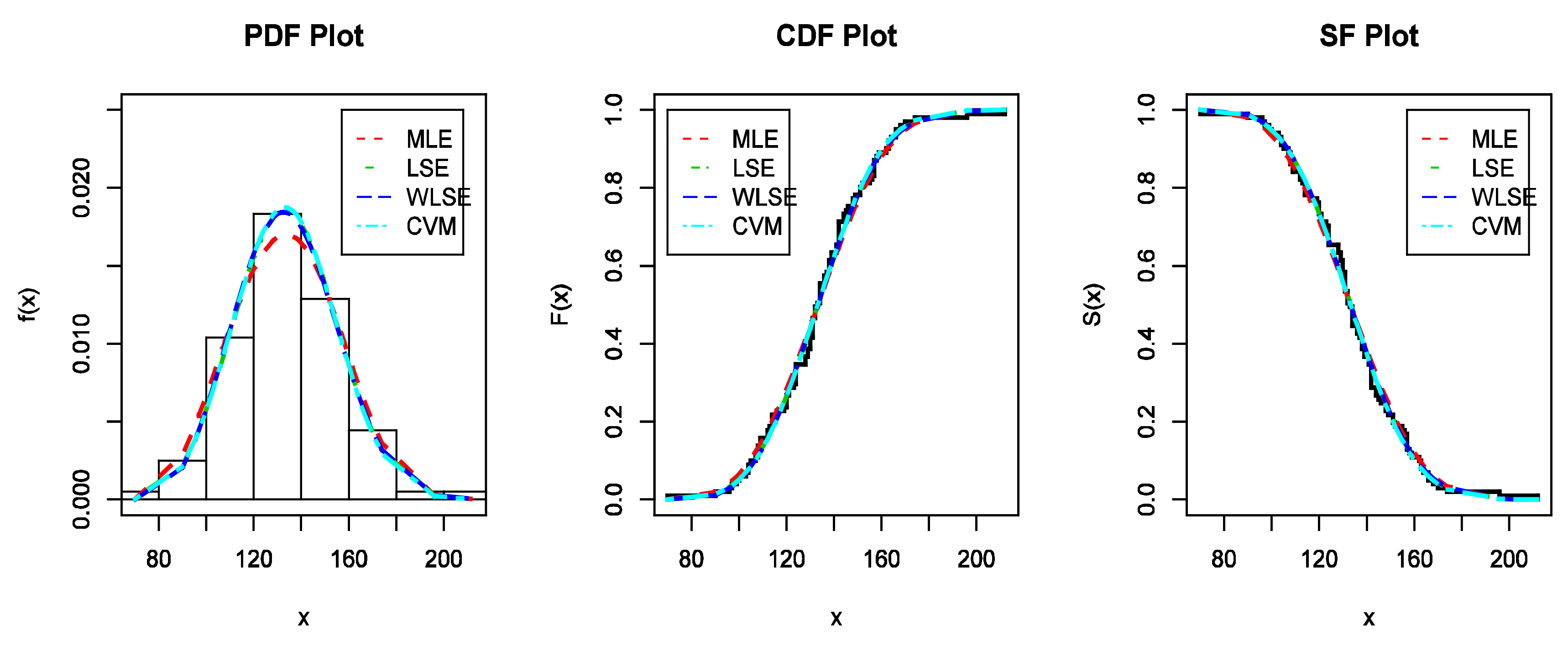
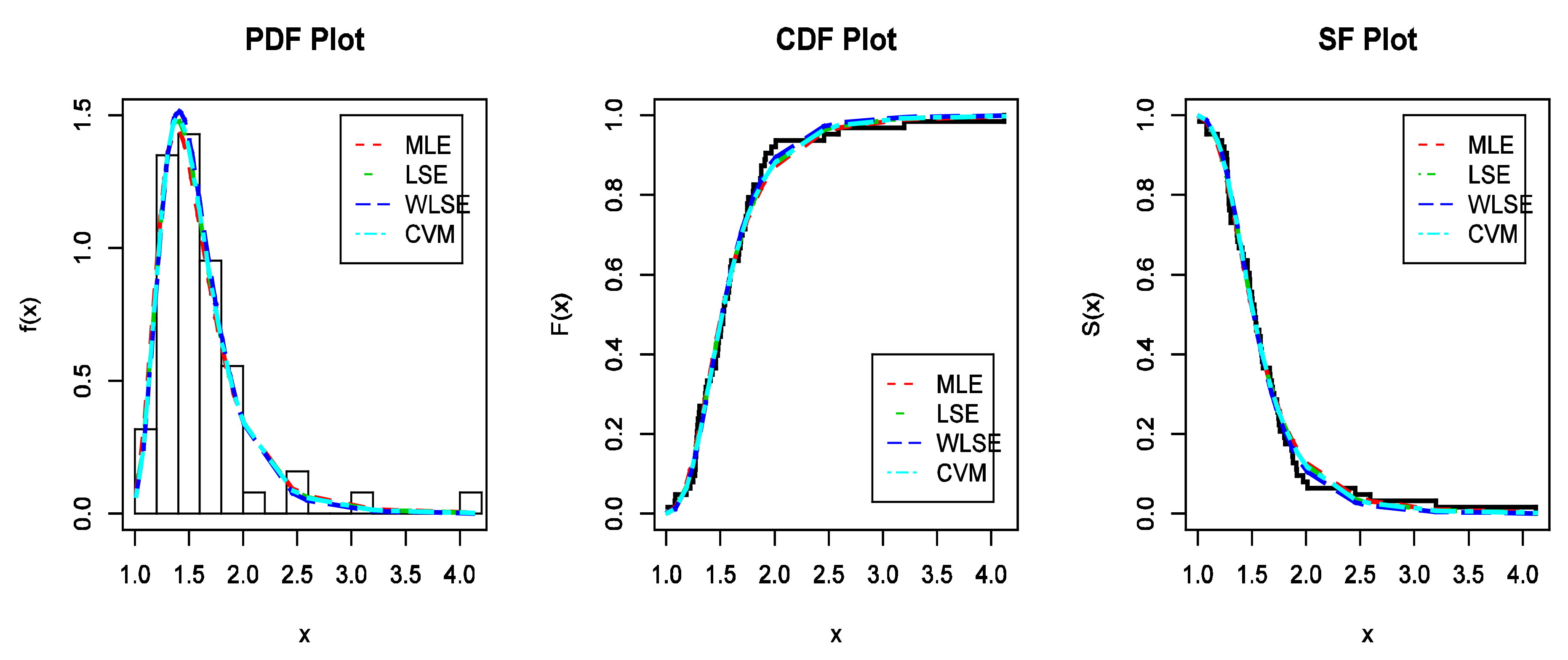
Figure 7.
The estimated PDFs, the estimated CDFs, and the estimated SFs for data I.
Figure 7.
The estimated PDFs, the estimated CDFs, and the estimated SFs for data I.
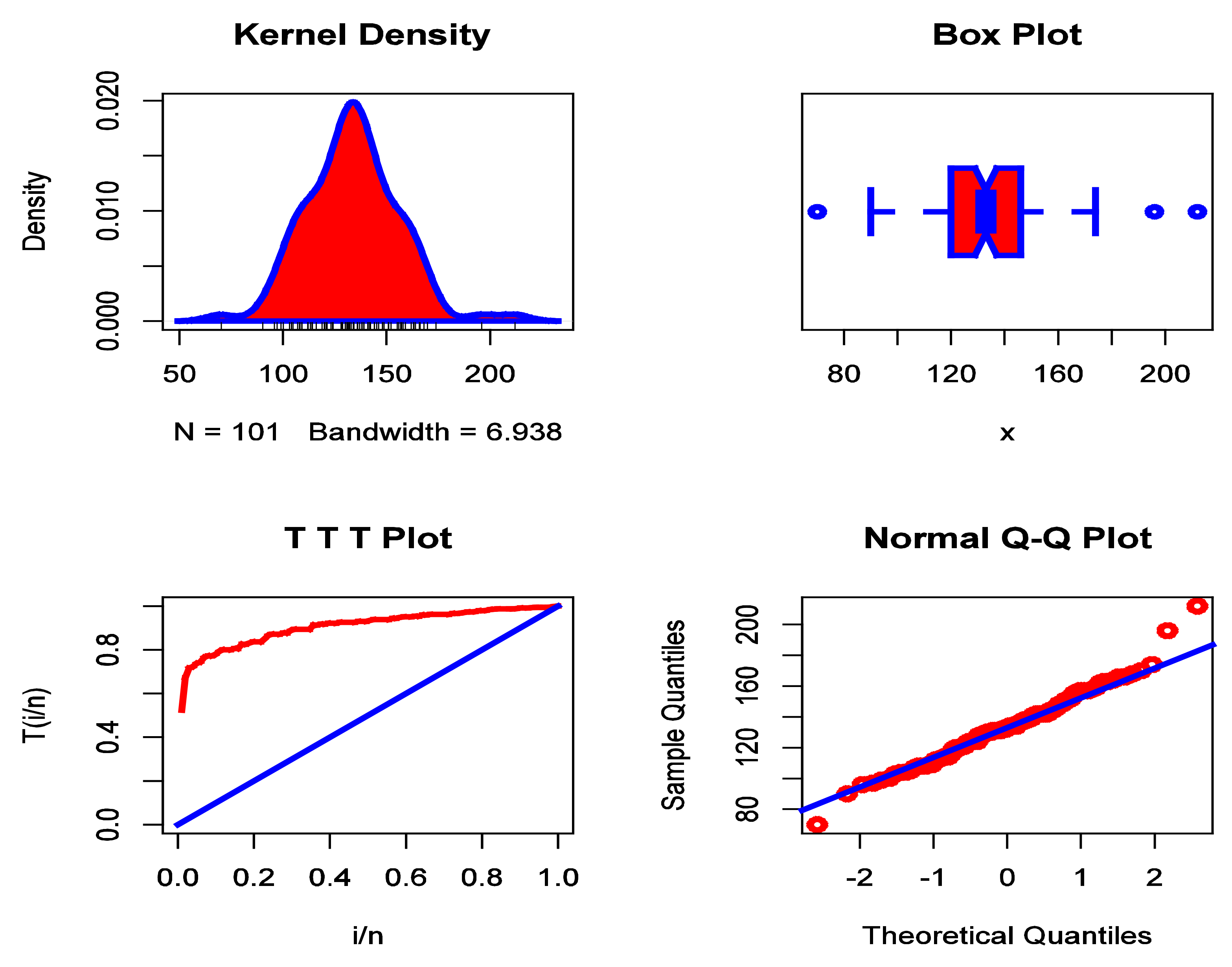
Figure 8.
The KDE plot, box plot, TTT plot, and Q–Q plot for data set II.
Figure 8.
The KDE plot, box plot, TTT plot, and Q–Q plot for data set II.
Figure 9.
The estimated PDF, P–P plot, estimated CDF, and estimated SF for data set II.
Figure 9.
The estimated PDF, P–P plot, estimated CDF, and estimated SF for data set II.
Figure 10.
The estimated PDFs, the estimated CDFs, and the estimated SFs for data set II.
Figure 10.
The estimated PDFs, the estimated CDFs, and the estimated SFs for data set II.
Figure 11.
The KDE plot, box plot, TTT plot, and Q–Q plot for data set III.
Figure 11.
The KDE plot, box plot, TTT plot, and Q–Q plot for data set III.
Figure 12.
The estimated PDF, P–P plot, estimated CDF, and the estimated SF for data set III.
Figure 12.
The estimated PDF, P–P plot, estimated CDF, and the estimated SF for data set III.
Figure 13.
The estimated PDFs, the estimated CDFs, and the estimated SFs for data set III.
Figure 13.
The estimated PDFs, the estimated CDFs, and the estimated SFs for data set III.
Table 1.
The MLEs, K-S, p-values, –L, A*, and W* values for the first data set.
Table 1.
The MLEs, K-S, p-values, –L, A*, and W* values for the first data set.
| Statistics | Models |
|---|
| IW | EGIW | IE | IR | IFW | EIFW | A | EGA | IG | EGIG |
|---|
| 4.46 | 34.756 | 29.215 | 810.504 | 61.167 | 2.376 | 125.662 | –– | 1.249 | 64.009 |
| 4.655 | 0.637 | –– | –– | 0.086 | 0.164 | –– | 9.526 | 119.762 | 63.247 |
| –– | 94.688 | –– | –– | –– | 81.512 | –– | 3.909 | –– | 37.998 |
| –– | 3.759 | –– | –– | –– | –– | –– | 1.95 | –– | 0.18 |
| K-S | 0.146 | 0.124 | 0.477 | 0.325 | 0.146 | 0.136 | 0.162 | 0.145 | 0.139 | 0.123 |
| p-value | 0.482 | 0.678 | <0.001 | 0.002 | 0.479 | 0.567 | 0.354 | 0.485 | 0.538 | 0.690 |
| –L | 105.323 | 104.102 | 137.262 | 118.201 | 104.963 | 104.141 | 107.95 | 105.615 | 107.884 | 103.286 |
| W* | 0.083 | 0.077 | 0.074 | 0.075 | 0.078 | 0.074 | 0.122 | 0.085 | 0.118 | 0.056 |
| A* | 0.503 | 0.407 | 0.392 | 0.403 | 0.467 | 0.397 | 0.804 | 0.521 | 0.778 | 0.309 |
Table 2.
The MLE, LSE, WLSE and CVM estimators, KS, and p-values for data set I.
Table 2.
The MLE, LSE, WLSE and CVM estimators, KS, and p-values for data set I.
| Method | | | | | K-S | p-Value |
|---|
| MLE | 64.009 | 63.247 | 37.998 | 0.180 | 0.123 | 0.690 |
| LSE | 94.141 | 54.489 | 63.339 | 0.145 | 0.094 | 0.945 |
| WLSE | 91.462 | 55.085 | 63.959 | 0.147 | 0.090 | 0.963 |
| CVM | 89.188 | 56.341 | 64.313 | 0.149 | 0.098 | 0.929 |
Table 3.
The LRT, , and p-values for data set I.
Table 3.
The LRT, , and p-values for data set I.
| Models | Null Hypothesis
| | | p-Value |
|---|
| A | or | 9.328 | 3 | 0.025 |
| IG | or | 9.196 | 2 | 0.010 |
| EGA | or | 4.658 | 1 | 0.031 |
Table 4.
The MLEs, K-S, p-values, –L, A*, and W* values for the second data set.
Table 4.
The MLEs, K-S, p-values, –L, A*, and W* values for the second data set.
| Statistics | Models |
|---|
| IW | EGIW | IE | IR | IFW | EIFW | A | EGA | IG | EGIG |
|---|
| 3.28 | 106.236 | 129.933 | 1.64 | 295.466 | 78.792 | 705.55 | –– | 7.435 | 469.618 |
| 5.051 | 0.935 | –– | –– | 0.021 | 0.039 | –– | 94.472 | 501.775 | 175.869 |
| –– | 11.981 | –– | –– | –– | 58.724 | –– | 3.041 | –– | 258.604 |
| –– | 77.271 | –– | –– | –– | –– | –– | 6.17 | –– | 0.375 |
| K-S | 0.133 | 0.125 | 0.506 | 0.403 | 0.139 | 0.113 | 0.366 | 0.186 | 0.206 | 0.067 |
| p-value | 0.055 | 0.085 | < 0.001 | < 0.001 | 0.039 | 0.153 | < 0.001 | 0.002 | < 0.001 | 0.749 |
| –L | 475.186 | 466.602 | 595.547 | 530.197 | 476.101 | 465.265 | 517.597 | 482.509 | 494.448 | 458.896 |
| W* | 0.432 | 0.299 | 0.121 | 0.172 | 0.437 | 0.238 | 1.204 | 0.491 | 0.803 | 0.089 |
| A* | 2.493 | 1.694 | 0.689 | 0.975 | 2.548 | 1.349 | 7.025 | 2.851 | 4.707 | 0.593 |
Table 5.
The MLE, LSE, WLSE, and CVM estimators, K-S, and p-values for data set II.
Table 5.
The MLE, LSE, WLSE, and CVM estimators, K-S, and p-values for data set II.
| Method | | | | | K-S | p-Value |
|---|
| MLE | 469.618 | 175.869 | 258.604 | 0.375 | 0.067 | 0.749 |
| LSE | 515.696 | 121.802 | 225.434 | 0.632 | 0.057 | 0.897 |
| WLSE | 397.808 | 172.611 | 141.765 | 0.529 | 0.057 | 0.904 |
| CVM | 490.022 | 134.638 | 218.369 | 0.600 | 0.072 | 0.666 |
Table 6.
The LRT, and p-values for data set II.
Table 6.
The LRT, and p-values for data set II.
| Models | Null Hypothesis | | | p-Value |
|---|
| A | or | 117.402 | 3 | 0.0 |
| IG | or | 71.104 | 2 | 0.0 |
| EGA | or | 47.226 | 1 | 0.0 |
Table 7.
The MLEs, K-S, p-values, –L, A*, and W* values for the third data set.
Table 7.
The MLEs, K-S, p-values, –L, A*, and W* values for the third data set.
| Statistics | Models |
|---|
| IW | EGIW | IE | IR | IFW | EIFW | A | EGA | IG | EGIG |
|---|
| 6.498 | 1.161 | 1.526 | 2.233 | 3.732 | 4.169 | 2.111 | –– | 0.032 | 0.495 |
| 5.438 | 3.529 | –– | –– | 1.869 | 1.666 | –– | 1.54 | 7.583 | 3.761 |
| –– | 1.731 | –– | –– | –– | 0.544 | –– | 6.249 | –– | 3.656 |
| –– | 8.139 | –– | –– | –– | –– | –– | 7.331 | –– | 1.461 |
| K-S | 0.077 | 0.071 | 0.468 | 0.36 | 0.082 | 0.084 | 0.521 | 0.069 | 0.101 | 0.068 |
| p-value | 0.819 | 0.889 | <0.001 | <0.001 | 0.756 | 0.739 | <0.001 | 0.904 | 0.508 | 0.916 |
| –L | 20.064 | 19.879 | 92.805 | 53.381 | 20.618 | 20.593 | 63.322 | 19.913 | 22.809 | 19.706 |
| W* | 0.071 | 0.062 | 0.126 | 0.087 | 0.079 | 0.081 | 0.063 | 0.059 | 0.138 | 0.061 |
| A* | 0.533 | 0.488 | 0.982 | 0.709 | 0.61 | 0.616 | 0.514 | 0.482 | 0.928 | 0.469 |
Table 8.
The MLE, LSE, WLSE, and CVM estimators, KS, and p-values for data set III.
Table 8.
The MLE, LSE, WLSE, and CVM estimators, KS, and p-values for data set III.
| Method | | | | | K-S | p-Value |
|---|
| MLE | 0.495 | 3.761 | 3.656 | 1.461 | 0.068 | 0.916 |
| LSE | 0.596 | 3.278 | 4.339 | 1.999 | 0.067 | 0.927 |
| WLSE | 0.847 | 2.722 | 5.856 | 2.369 | 0.075 | 0.866 |
| CVM | 0.589 | 3.300 | 4.363 | 2.031 | 0.072 | 0.898 |
Table 9.
The LRT, and p-values for data set III.
Table 9.
The LRT, and p-values for data set III.
| Models | Null Hypothesis | | | p-Value |
|---|
| A | or | 87.232 | 3 | 0.0 |
| IG | or | 6.206 | 2 | 0.045 |
| EGA | or | 0.414 | 1 | 0.519 |
Table 10.
The MLEs, –L, K-S, and p-values for data set V.
Table 10.
The MLEs, –L, K-S, and p-values for data set V.
| Models | MLEs | –L | K-S | p-Value |
|---|
| A | | 7.592 | 0.687 | 0.046 |
| IG | | 3.25 | 0.513 | 0.285 |
| EGA | | 2.992 | 0.479 | 0.319 |
| EGIG | | 2.873 | 0.469 | 0.341 |


