AMT Starting Control as a Soft Starter for Belt Conveyors Using a Data-Driven Method

Abstract

Automated mechanical transmission (AMT) is used as a soft starter in this paper. To improve the soft starting quality, a novel data-driven method is studied. By analyzing and comparing five common soft-starting acceleration curves, a segmented acceleration curve is put forward to be used as the soft-starting acceleration curve for the AMT. Based on the prototype model free adaptive control (MFAC) method, a modified MFAC method with jerk compensation is given to control the AMT output shaft’s angular acceleration and reduce driveline shock. Compared with the methods of prototype MFAC and traditional proportion integration differentiation (PID), the modified MFAC method with jerk compensation can better control the AMT output shaft’s angular acceleration and has excellent characteristics in terms of small tracking error and smaller shock. The research results provide a novel data-driven method for AMT as a soft starter.

1. Introduction

In recent decades, the belt conveyors have come to play an important role for the dry bulk material transport. The conveyor belt is composed of rubber, fiber, and metal, with viscoelastic properties and complicated dynamic characteristics [1,2,3,4]. As has been acknowledged, the vibration of the conveyor belt may cause serious accidents, such as belt breaking, belt slipping, and belt wear for long-distance and high-power belt conveyors during their starting process [5,6,7,8]. These asymmetric malicious problems will occur if the technical difficulties during the starting process cannot be resolved, while symmetric phenomena will appear if the problems with technologies during the starting process can be dealt well. Therefore, softly starting the belt conveyors is very important. Many scholars have proposed some “S” style speed curves. From the available literatures, five soft-starting acceleration curves exist for belt conveyors, including the constant acceleration curve, the sine acceleration curve, the triangle acceleration, the trapezoidal acceleration, and the parabola acceleration [9,10]. A reasonable acceleration starting curve can decrease belt vibration and belt accidents.

Currently, the common soft starters for belt conveyors include the variable frequency and hydro-viscous drives. The principle of variable frequency drives is to adjust their frequency with change in motor speed [11]. Hydro-viscous drives mainly use a wet clutch to change the speed difference between the active and driven plates [12,13,14,15]. The variable frequency drives are used in dry locations with sufficient ventilation for the use requirements of the electrical equipment. The hydro-viscous drives are used in cleaning and in airy places for their high-quality oil and high maintenance costs. The above soft starters cannot be widely used in contexts such as mining, due to the associated high price and high maintenance cost.

AMT has been widely used in heavy-duty trucks for two decades for its advantages of low price, low maintenance cost, and high efficiency [16,17,18]. We propose its use as a new soft starter for medium-scale belt conveyors with 400 kW in this paper, as its maximum input torque can reach 3400 N·m, as provided by ZF Friedrichshafen AG. Soft-starting theory through gradual shifting is elaborated in the author’s published papers [19,20].

Figure 1 illustrates the AMT soft-starting system. The AMT soft-starting system includes a three-phase asynchronous motor, an AMT, a reducer, and a belt conveyor. The AMT control system consists of a transmission control unit (TCU), several sensors and several actuators. Heavy-duty AMT is generally composed of a main gearbox and an auxiliary gear box, which has ten or more forward gears. The main gear box is a traditional mechanical transmission controlled by selecting and shifting actuators and the auxiliary gearbox is a planetary gear set controlled by a range gear actuator.

The clutch combines or cuts the transfer of motivity by controlling the clutch engagement and disengagement. In particular, the clutch engagement process includes the empty, resistance, acceleration, and full engagement stages in this paper. Their tasks are eliminating the free clearance, overcoming the running resistance force, controlling the AMT output shaft’s angular acceleration, and separately maintaining a running speed under certain gear positions. The key stage is the acceleration stage in which the AMT output shaft’s angular acceleration can be controlled, and the conveyor belt can be started-up softly.

Describing the clutch’s torque transmissibility is difficult, due to the mechanical properties of the diaphragm spring and the nonlinear properties of the friction disk. The estimation methods of clutch torque have been studied in recent years [21,22,23]. Clutch torque transmissibility can be considered to have nonlinear characteristics. Moreover, the clutch actuator has some hysteresis characteristics. In practice, controlling the AMT output shaft’s angular acceleration to accurately track the ideal given curve is difficult.

The speed signal of the AMT output shaft changes slowly if the output shaft speed is lower than 20 rpm. Therefore, control methods based on models are not suitable for clutch control. Data-driven control methods have better control performances for complicated and nonlinear actuators, thereby eliminating the need to build an accurate mathematical model. Depending only on the input and output data, data-driven control methods can achieve adaptive control for these complicated and nonlinear actuators. Some data-driven control methods, such as proportion integration differentiation (PID), fuzzy PID, active disturbance rejection control (ADRC), iterative learning control (ILC), and prototype model free adaptive control (MFAC) have been widely used in industrial control [24,25,26,27]. Hou proposed the MFAC method, which features better control characteristics with good tracking performance [28,29,30,31]. In this paper, it is selected as the basic method for controlling the AMT output shaft’s angular acceleration in order to better control the belt acceleration for the belt conveyor’s soft starting.

The belt shock will occur significantly if the AMT output shaft’s angular jerk exceeds a certain threshold. To avoid a dangerous outcomes, the AMT output shaft’s angular jerk should be restricted. Therefore, a modified MFAC method with jerk compensation is proposed as the optimal control method to better control the AMT output shaft’s angular acceleration for the AMT as a soft starter.

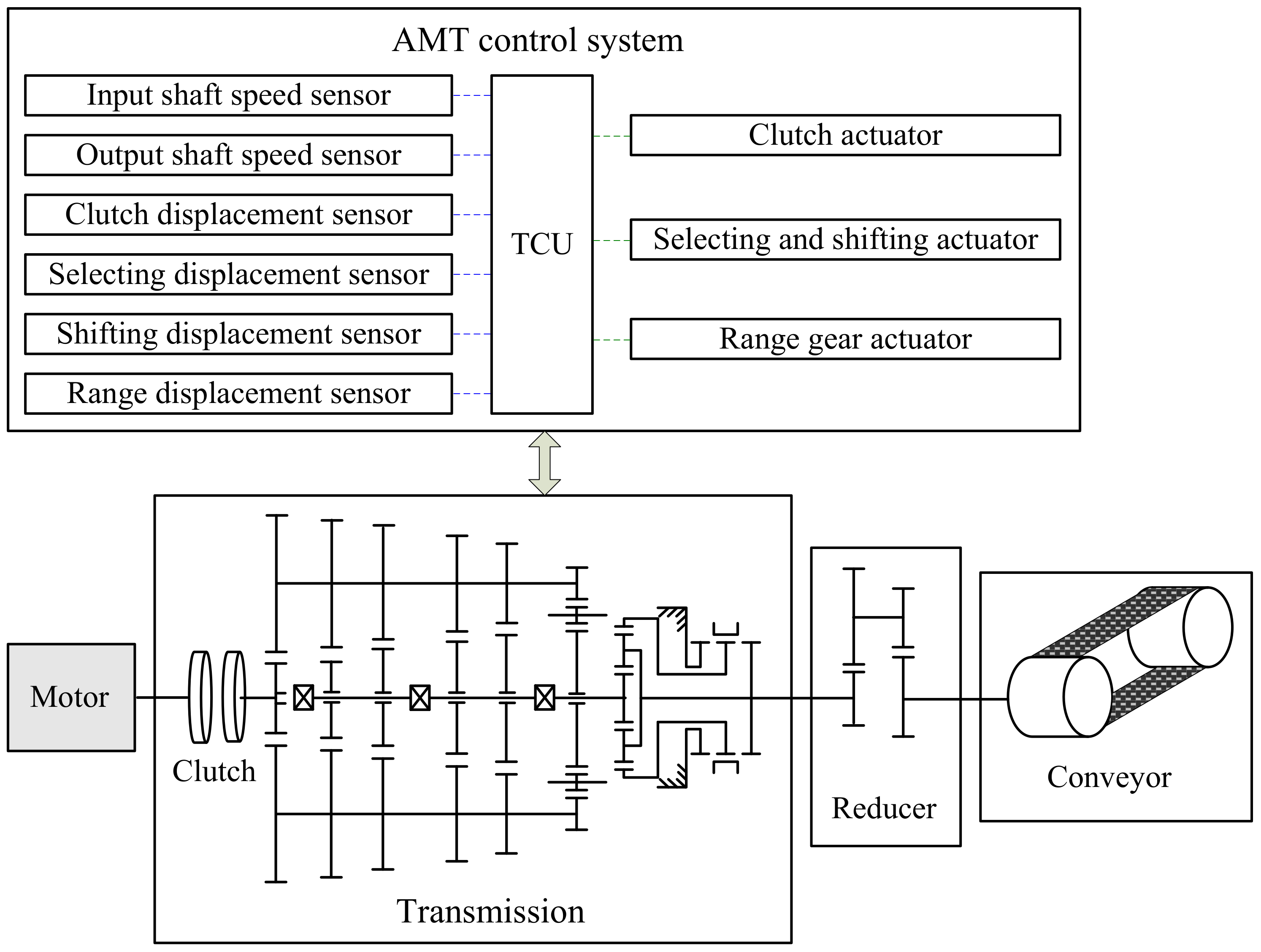
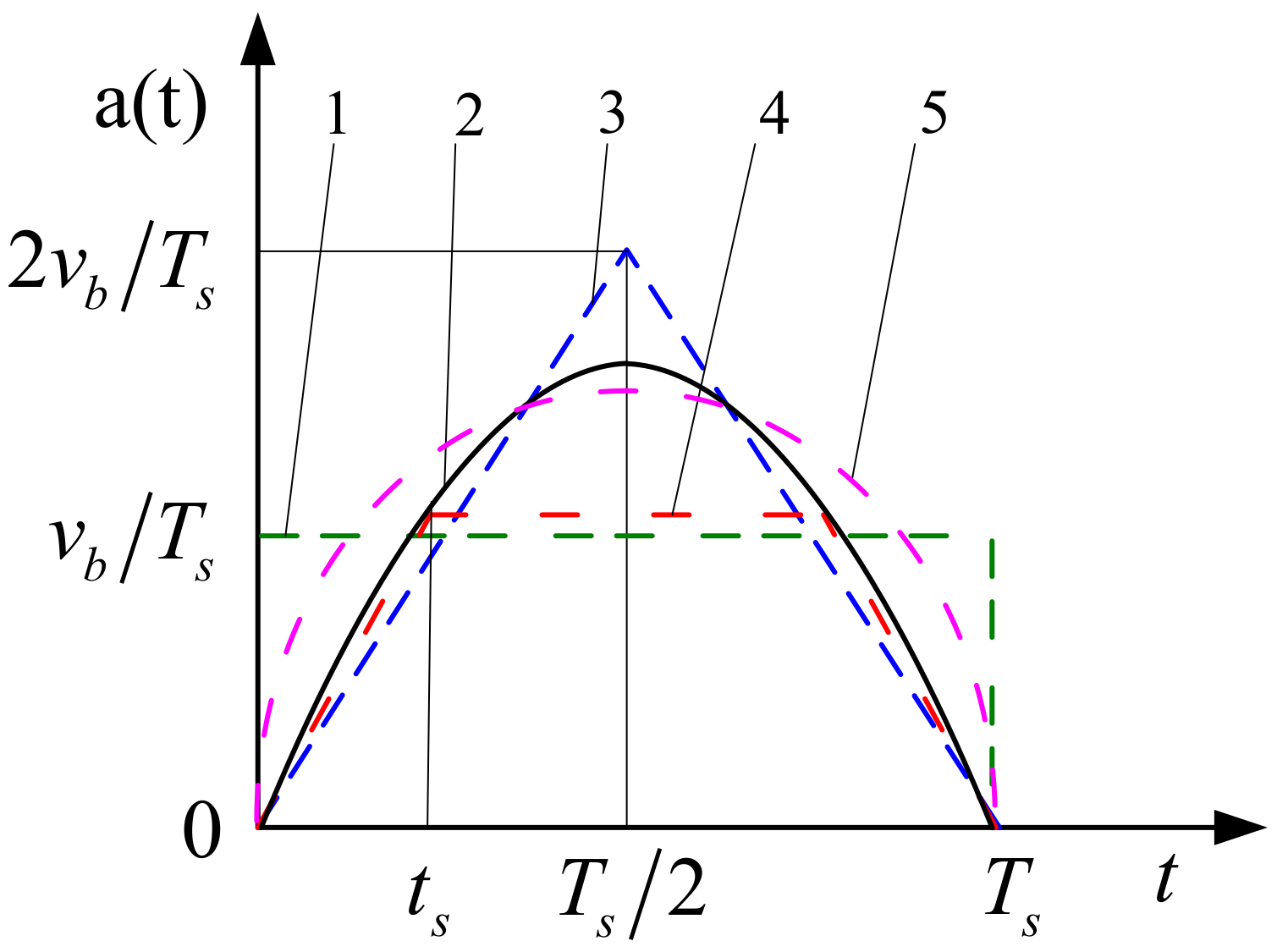
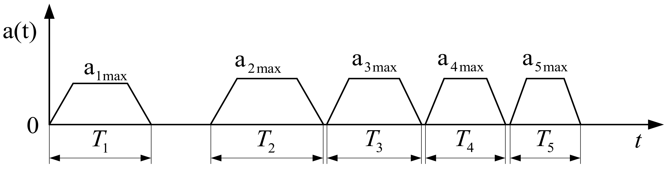
2. Starting Acceleration Curve Based on AMT

The common starting acceleration expressions are illustrated below.

The constant acceleration curve can be expressed as:

$$\begin{array}{cc}a\left(t\right)=\frac{1}{T_s}{v}_b& \left(0\le t\le T_s\right)\end{array}$$

(1)

where v_b is the belt target speed, T_s is the starting time.

The sine acceleration curve is given by:

$$\begin{array}{cc}a\left(t\right)=\frac{\pi }{2T_s}{v}_b\sin \left(\frac{\pi }{T_s}t\right)& \left(0\le t\le T_s\right)\end{array}$$

(2)

The triangular acceleration curve is:

$$a\left(t\right)=\left\{\begin{array}{ll}4v_b\frac{t}{T_s^2}\hfill & (0\le t\le T_s/2)\hfill \\ 4v_b\left(\frac{1}{T_s}-\frac{t}{T_s^2}\right)\hfill & (T_s/2<t\le T_s)\hfill \end{array}\right.$$

(3)

The trapezoidal acceleration curve is:

$$a\left(t\right)=\left\{\begin{array}{ll}\frac{v_b}{\left(N-1\right)t_s^2}t\hfill & \left(0\le t\le t_s\right)\hfill \\ \frac{N{v}_b}{\left(N-1\right)T_s}\hfill & (t_s<t<T_s-t_s)\hfill \\ \frac{N^2{v}_b}{\left(N-1\right)T_s^2}\left(T_s-t\right)\hfill & \left(T_s-t_s\le t\le T_s\right)\hfill \end{array}\right.$$

(4)

where N is a natural number greater than 3, t_s is the time of the ascent or descent acceleration stage, t_s is equal to T_s divided by N.

The parabolic acceleration curve is:

$$\begin{array}{cc}a\left(t\right)=6v_b\left(\frac{t}{T_s^2}-\frac{t^2}{T_s^3}\right)& \left(0\le t\le T_s\right)\end{array}$$

(5)

Under the same starting time, Figure 2 presents the schematic of the above five common starting acceleration curves.

Table 1. Comparisons of characteristic parameters for the common starting curves.

Type	Time	Velocity	Acceleration	Jerk
Constant acceleration	0	0	vb/Ts	∞
	Ts	vb	vb/Ts	−∞
Sine acceleration	0	0	0	${\pi }^2{v}_b/\left(2T_s^2\right)$
	Ts/2	vb/2	$\pi v_b/\left(2T_s\right)$	0
	Ts	vb	0	$-{\pi }^2{v}_b/\left(2T_s^2\right)$
Triangular acceleration	0	0	0	$4v_b/T_s^2$
	Ts/2	vb/2	$2v_b/T_s$	$4v_b/T_s^2$
	Ts	vb	0	$-4v_b/T_s^2$
Trapezoidal acceleration	0	0	0	$\frac{N^2{v}_b}{\left(N-1\right)T_s^2}$
	$\frac{T_s}{N}$	$\frac{v_b}{2\left(N-1\right)}$	$\frac{N{v}_b}{\left(N-1\right)T_s}$	$\frac{N^2{v}_b}{\left(N-1\right)T_s^2}$
	$\frac{\left(N-1\right)T_s}{N}$	$\frac{\left(2N-3\right)v_b}{2\left(N-1\right)}$	$\frac{N{v}_b}{\left(N-1\right)T_s}$	0
	Ts	vb	0	$-\frac{N^2{v}_b}{\left(N-1\right)T_s^2}$
Parabola acceleration	0	0	0	$6v_b/T_s^2$
	Ts/2	vb/2	$3v_b/\left(2T_s\right)$	0
	Ts	vb	0	$-6v_b/T_s^2$

lists the comparisons of the characteristic parameters including the belt velocity, the belt acceleration, and the belt jerk (the differential of the acceleration).

From the perspective of peak acceleration, those of the triangular, sine, and constant acceleration curves occupy the first, second, and last places, respectively. From the perspective of peak jerk, those of the triangular, sine, and constant acceleration curves are described as the smallest, middling, and greatest, respectively. The greater the peak jerk, the greater the belt vibration. Therefore, the sine and triangular acceleration curves are generally chosen for soft starters.

To meet the requirements of the belt conveyor’s soft starting, studying which acceleration curve is more suitable for AMT is necessary. To reduce clutch wear, seeking to reduce starting time is reasonable. The acceleration algorithm should not be excessively complicated, due to the hysteresis properties of the AMT actuators. Following the above analysis, the triangular and trapezoidal acceleration curves are practicable in reducing starting time and peak jerk. Belt acceleration is achieved by controlling the duty ratios of the clutch-engaging solenoid valve and the clutch-disengaging solenoid valve. Combing the above analysis, a segmented acceleration curve is proposed to control the acceleration process for AMT as a soft starter, as shown in Figure 3.

The segmented acceleration curve can be illustrated as follows. It comprises several trapezoidal acceleration curves, determined by the belt speed and gear positions. The first stage of the conveyor’s starting process is to accelerate the belt from zero to the target speed under the first gear position, which is labeled T₁ and kept running at its target speed for longer than 5 s to stretch the entire belt. Then, the clutch should be disengaged and the gear position shifted to the second gear position. The second stage of the conveyor’s starting process is to continue accelerating the belt from the previous speed to the target speed under the second gear position which is labeled T₂ and kept running at its speed for 2 s. Then, the clutch should be disengaged again and the gear position shifted to the third gear position. The third stage of the conveyor’s starting process continues accelerating, labeled T₃, and kept running at its speed for 2 s. Similarly, the other stages are completed through upshifting until the target belt speed is reached. Finally, the conveyor’s soft starting process is completed.

3. AMT Dynamics Analysis

3.1. Clutch Torque Transmissibility

The clutch-transmitted torque can be expressed as a third-order polynomial concerning the big-end displacement of the diaphragm spring [32,33,34]. The clutch actuator is an air cylinder controlled by the solenoid valves, and the piston displacement is proportional to the big-end displacement of the diaphragm spring. Therefore, the clutch-transmitted torque can also be expressed as a third-order polynomial concerning the clutch actuator displacement. Normally, the clutch friction disk is often worn which will affect the clutch’s torque transmissibility. Therefore, the clutch-transmitted torque can be expressed as:

$$T_c\left(x\right)={\mu }^{\prime }\left[K_1\left(x-x_0-\Delta x_0\right)+K_2{\left(x-x_0-\Delta x_0\right)}^2+K_3{\left(x-x_0-\Delta x_0\right)}^3\right]$$

(6)

where 𝜇^′ is the friction coefficient of the clutch disk, x is the clutch actuator displacement, x₀ is the clutch actuator displacement at the critical point of the empty stroke for the new clutch, Δx₀ is the displacement increment of the clutch’s empty stroke due to wearing.

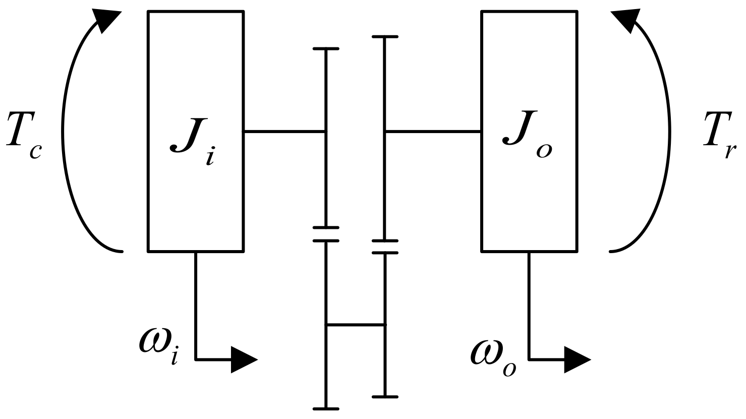
3.2. Transmission Dynamic Model

The input and output shafts can be regarded as two mass units. Thus, the transmission model can be built as a double-mass model, as shown in Figure 4.

Assuming the system damping is ignored, the transmission dynamic equation can be expressed as:

$$\left\{\begin{array}{l}\begin{array}{l}{\dot{\omega }}_o=\frac{T_c\left(x\right)i_g{i}_g-T_r}{J_i{i}_g^2+J_o}\hfill \\ {\ddot{\omega }}_o=\frac{d{\dot{\omega }}_o}{dt}\hfill \end{array}\hfill \\ \begin{array}{l}{T}_c\left(x\right)={\mu }^{\prime }\left[K_1\left(x-x_0-\Delta x_0\right)+K_2{\left(x-x_0-\Delta x_0\right)}^2+K_3{\left(x-x_0-\Delta x_0\right)}^3\right]\hfill \\ T_r=\frac{F_f{r}_d}{i_r{\eta }_r}\hfill \end{array}\hfill \\ J_o=J_t+\frac{J_c+J_r}{i_r^2}\hfill \end{array}\right.$$

(7)

where J_i, J_t, J_c, and J_r are the moment of inertia about the AMT input shaft, AMT output shaft, belt conveyor, and reducer’s output shaft, respectively. J_o is the equivalent moment of inertia about the AMT output shaft. 𝜔_i and 𝜔_o are the AMT input and output shaft’s angular speeds, respectively. ${\dot{\omega }}_o$ and ${\ddot{\omega }}_o$ are the AMT output shaft’s angular acceleration and jerk, respectively. T_c(x) and T_r are the transmitted torque of the clutch and the equivalent resistance torque of the AMT output shaft, respectively. F_f is the running resistance force of the belt conveyor. r_d is the head roller’s radius of the belt conveyor. i_g and i_r are the transmission ratio and the reducer ratio. ${\eta }_g$ and ${\eta }_r$ are the AMT efficiency and the reducer efficiency, respectively.

If the sampling interval is T, the discrete model of Equation (7) can be written:

$$\left\{\begin{array}{c}{\omega }_o\left(k+1\right)={\omega }_o\left(k\right)+T\frac{T_c\left(x\left(k\right)\right)i_g{\eta }_g-T_r\left(k\right)}{\left(J_i{i}_g^2+J_o\left(k\right)\right)}\hfill \\ {\ddot{\omega }}_o\left(k\right)=\frac{{\dot{\omega }}_o\left(k\right)-{\dot{\omega }}_o\left(k-1\right)}{T}\hfill \\ T_c\left(x\left(k\right)\right)={\mu }^{\prime }\left[K_1\left(x\left(k\right)-x_0-\Delta x_0\right)+K_2{\left(x\left(k\right)-x_0-\Delta x_0\right)}^2+K_3{\left(x\left(k\right)-x_0-\Delta x_0\right)}^3\right]\hfill \\ T_r\left(k\right)=\frac{F_{f\left(k\right)}{r}_d}{i_r{\eta }_r}\hfill \\ J_o\left(k\right)=J_t+\frac{J_c\left(k\right)+J_r}{i_r^2}\hfill \end{array}\right.$$

(8)

where k is a natural number. ${\omega }_o\left(k\right)$ and ${\omega }_o\left(k+1\right)$ are the angular speed at No. k sampling time and that at No. (k + 1) sampling time separately. ${\dot{\omega }}_o\left(k-1\right)$ and ${\dot{\omega }}_o\left(k\right)$ are the AMT output shaft’s angular accelerations at No. (k − 1) and No. k sampling times. ${\ddot{\omega }}_o\left(k\right)$ is the AMT output shaft’s angular jerk at No. k sampling time.

3.3. Angular Acceleration Curve of the AMT Output Shaft

The equivalent angular acceleration curve of the AMT output shaft is given in Equation (9) according to Equation (4).

$${\dot{\omega }}_o\left(t\right)=\left\{\begin{array}{ll}\frac{i_r{v}_b}{r_d\left(N-1\right)t_s^2}t\hfill & \left(0\le t\le t_s\right)\hfill \\ \frac{i_{r}N{v}_b}{r_d\left(N-1\right)T_s}\hfill & \left(t_s\le t\le T_s-t_s\right)\hfill \\ \frac{i_r{N}^2{v}_b}{r_d\left(N-1\right)T_s^2}\left(T_s-t\right)\hfill & (T_s-t_s\le t\le T_s)\hfill \end{array}\right.$$

(9)

4. Acceleration Control Method

The ascent stage of the trapezoidal acceleration curve can be achieved by controlling the duty ratios of the engaging solenoid valve and closing the disengaging solenoid valve. Moreover, the descent stage of the trapezoidal acceleration curve can be accomplished by controlling the duty ratios of the disengaging solenoid valve and closing the engaging solenoid valve. The horizontal stage of the trapezoidal acceleration curve can be accomplished by closing the engaging and disengaging solenoid valves. Based on the prototype MFAC method, the modified MFAC method with jerk compensation is proposed as follows: it is used not only to control the AMT output shaft’s angular acceleration but also to reduce the potential shocks during AMT’s starting and shifting.

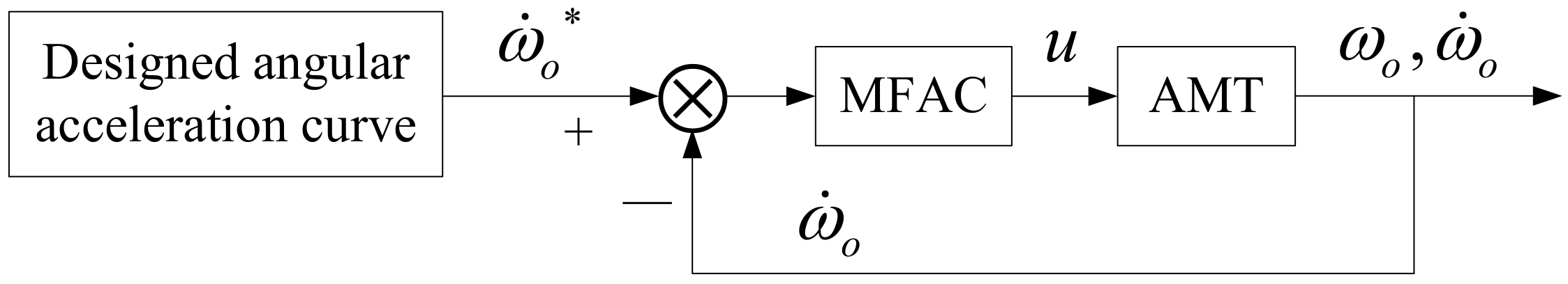
4.1. Prototype MFAC Method

Figure 5 presents the block diagram of the prototype MFAC method. Given by the designed angular acceleration curve of the AMT output shaft, the MFAC controller controls the duty ratio u of the clutch solenoid valve to control the clutch displacement. Thus, the AMT output shaft’s angular acceleration ${\dot{\omega }}_o$ can be regulated to trace the ideal angular acceleration ${\dot{\omega }}_o{}^{*}$.

The discrete algorithm of the AMT output shaft’s angular acceleration can be expressed by:

$${\dot{\omega }}_o\left(k+1\right)=\frac{1}{T}\left({\omega }_o\left(k+1\right)-{\omega }_o\left(k\right)\right)$$

(10)

where ${\dot{\omega }}_o\left(k+1\right)$ is the AMT output shaft’s angular acceleration at No. (k + 1) sampling time.

The AMT system can be regarded as a dynamic linear model using the MFAC theory which is driven by data in Equation (11):

$$\left\{\begin{array}{l}\Delta {\dot{\omega }}_o\left(k+1\right)={\varphi }_c\left(k\right)\mathsf{\Delta }u\left(k\right)\hfill \\ \mathsf{\Delta }{\dot{\omega }}_o\left(k+1\right)={\dot{\omega }}_o\left(k+1\right)-{\dot{\omega }}_o\left(k\right)\hfill \\ \mathsf{\Delta }u\left(k\right)=u\left(k\right)-u\left(k-1\right)\hfill \end{array}\right.$$

(11)

where ${\varphi }_c\left(k\right)$ is the pseudo partial derivative (PPD) of the system at No. k sampling time which is not equal to zero, ${\dot{\omega }}_o\left(k\right)$ is the AMT output shaft’s angular acceleration at No. k sampling time, ${\dot{\Delta \omega }}_o\left(k+1\right)$ is the increment of the AMT output shaft’s angular acceleration at No. (k + 1) sampling time, u(k) and u(k − 1) are the duty ratios of the solenoid valve at No. k sampling time and that at No. (k − 1) sampling time separately.

The weighting square sum based on the forward prediction errors is used as the criterion function to control the input parameter in Equation (12).

$$J\left(u\left(k\right)\right)={\left({\dot{\omega }}_o{}^{*}\left(k+1\right)-{\dot{\omega }}_o\left(k+1\right)\right)}^2+\lambda {\left(u\left(k\right)-u\left(k-1\right)\right)}^2$$

(12)

where 𝜆 is a weighting factor which is more than zero to limit the input parameter u(k), ${\dot{\omega }}_o{}^{*}\left(k+1\right)$ is the ideal angular acceleration given by the designed angular acceleration curve at No. (k + 1) sampling time.

Taking the derivative of Equation (12) with respect to u(k) and letting its value be equal to zero, the control algorithm of u(k) is obtained in Equation (13).

$$u\left(k\right)=u\left(k-1\right)+\frac{\rho {\varphi }_c\left(k\right)\left({\dot{\omega }}_o{}^{*}\left(k+1\right)-{\dot{\omega }}_o\left(k\right)\right)}{\lambda +{\varphi }_c^2\left(k\right)}$$

(13)

where 𝜌 is a step factor which is more than zero and less than or equal to 1 to adjust the increment of Δu(k).

The estimation criterion function about ${\varphi }_c\left(k\right)$ can be expressed as:

$$J\left({\varphi }_c\left(k\right)\right)={\left({\dot{\omega }}_o\left(k\right)-{\dot{\omega }}_o\left(k-1\right)-{\varphi }_c\left(k\right)\mathsf{\Delta }u\left(k-1\right)\right)}^2+\mu {\left({\varphi }_c\left(k\right)-{\widehat{\varphi }}_c\left(k-1\right)\right)}^2$$

(14)

where 𝜇 is a penalty factor which is more than zero to limit the changes of ${\varphi }_c\left(k\right)$.

Taking the derivative of Equation (14) with respect to ${\varphi }_c\left(k\right)$ and letting its value be equal to zero, which means to minimize the estimation criterion function expressed by Equation (14), then the estimation algorithm of ${\widehat{\varphi }}_c\left(k\right)$ is obtained in Equation (15).

$$\left\{\begin{array}{l}{\widehat{\varphi }}_c\left(k\right)={\widehat{\varphi }}_c\left(k-1\right)+\frac{\eta \mathsf{\Delta }u\left(k-1\right)}{\mu +{\left(\mathsf{\Delta }u\left(k-1\right)\right)}^2}\left(\mathsf{\Delta }{\dot{\omega }}_o\left(k\right)-{\widehat{\varphi }}_c\left(k-1\right)\mathsf{\Delta }u\left(k-1\right)\right)\hfill \\ \mathsf{\Delta }{\widehat{\varphi }}_c\left(k\right)={\widehat{\varphi }}_c\left(k\right)-{\widehat{\varphi }}_c\left(k-1\right)\hfill \end{array}\right.$$

(15)

where 𝜂 is a step factor which is more than zero and less than or equal to 1 to adjust the increment of $\mathsf{\Delta }{\widehat{\varphi }}_c\left(k\right)$.

To make the parameters estimation algorithm achieve a good time-tracking feature, the relevant parameters are reset in Equation (16):

$$\left\{\begin{array}{l}{\widehat{\varphi }}_c\left(k\right)={\widehat{\varphi }}_c\left(1\right)\hfill \\ \begin{array}{l}if \left|{\widehat{\varphi }}_c\left(k\right)\right|\le \epsilon \hfill \\ or \left|\Delta u\left(k-1\right)\right|\le \epsilon \hfill \end{array}\hfill \\ or sign\left({\widehat{\varphi }}_c\left(k\right)\right)\ne sign\left({\widehat{\varphi }}_c\left(1\right)\right)\hfill \end{array}\right.$$

(16)

where ${\widehat{\varphi }}_c\left(1\right)$ is an initial value of ${\widehat{\varphi }}_c\left(k\right)$, $\epsilon$ is a very small positive number which provides the flexibility for ${\widehat{\varphi }}_c\left(k\right)$ and Δu(k − 1).

If Δu(k − 1) equals zero at No. k − 1 sampling time, the time should be moved backward until u(k − 1) is not equal to u(k − m) at No. (k − m) sampling time. Therefore, the system can be transformed into a dynamic linear model based on Equation (15).

To summarize, the algorithm of the prototype MFAC method comprises Equations (13), (15), and (16).

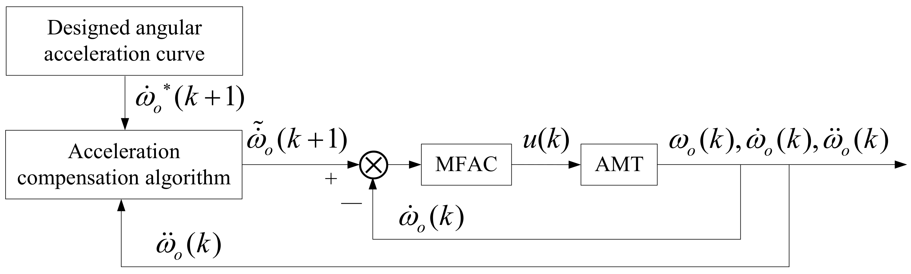
4.2. MFAC Method with Jerk Compensation

The AMT output shaft’s angular jerk is defined as the change of the AMT output shaft’s angular acceleration per unit time. The jerk compensation is used to improve the soft starting quality if the absolute value of the jerk exceeds the set threshold. Figure 6 presents the block diagram of the modified MFAC method with jerk compensation.

The jerk compensation algorithm can be described by:

$${\tilde{\dot{\omega }}}_o\left(k+1\right)={\dot{\omega }}_o{}^{*}\left(k+1\right)\pm \xi \frac{\left(\left|{\ddot{\omega }}_o\left(k\right)\right|-{\ddot{\omega }}_{omax}\right)}{{\ddot{\omega }}_{omax}}{\dot{\omega }}_o{}^{*}\left(k+1\right)$$

(17)

where 𝜉 is a weighting factor which is greater than zero and less than 1, ${\tilde{\dot{\omega }}}_o\left(k+1\right)$ is the modified ideal angular acceleration of the AMT output shaft at No. k sampling time, $\left|{\ddot{\omega }}_o\left(k\right)\right|$ is the absolute value of the AMT output shaft’s angular jerk at No. k sampling time, ${\ddot{\omega }}_{omax}$ is the set threshold. “−” and “+” are used during the ascent and descent acceleration stages, respectively.

Now, the algorithm of the modified MFAC method with jerk compensation for AMT is given by including Equations (13), (15)–(17).

5. Simulation and Analysis

To prove whether the modified MFAC method with jerk compensation is efficient for soft starting, simulation experiments were thoroughly studied under the first gear position and compared with the prototype MFAC method, the modified MFAC method with jerk compensation, and the PID method.

5.1. Driveline Parameters

A belt conveyor with a driving power of 4 × 315 kW is shown in Figure 7. The task is to transport coal from a mine to a coal storage bunker above ground. It has a coal transportation volume of 3500 tons per hour and has a length of 8460 m. It needs four three-phased asynchronous motors and four soft starters.

The basic parameters of the driveline are described below. The power of the three-phase asynchronous motor is 315 kW. The driven roller radius of the belt conveyor is 0.5 m. The motor rated speed is 1480 rpm. Calculating according to a quarter of the belt conveyor’s load, every driving system should carry an equivalent running mass of 248,696 kg and equivalent running resistance force of 50,819 N for the whole set of belt conveyors. The first gear ratio of AMT is 14.28. The transmission efficiency of AMT is approximately 0.96 (The value can be found from the AMT provided by ZF cooperation). The equivalent moment of inertia about the AMT output shaft is 10 kg·m². The moment of inertia about the clutch active parts (the pressure plate and the flywheel) and that of the clutch disk are 1.3 kg·m² and 0.135 kg·m², respectively. The transmission efficiency of the reducer is approximately 0.97.

If x_d is the big-end displacement of the diaphragm spring, the transmitted torque of the clutch is a function about the big-end displacement of the diaphragm spring in the literature [35], which can be expressed as:

$$T_c={\mu }^{\prime }\left(3464.483459x_d-336.521878x_d{}^2+7.775271x_d{}^3\right)$$

(18)

If the friction coefficient 𝜇′ equals 0.25, the lever ratio between the clutch actuator displacement and the big-end displacement of the diaphragm spring is six, the value of x₀ is 10 mm, and x(k) is the clutch actuator displacement at No. k sampling time. Then, the discrete model of the transmitted torque of the new clutch is expressed in Equation (19) according to Equation (6).

$$T_c\left(x\left(k\right)\right)=144.353477\left(x\left(k\right)-10\right)-2.336957{\left(x\left(k\right)-10\right)}^2+0.008999{\left(x\left(k\right)-10\right)}^3$$

(19)

The engaging solenoid valve can be fully closed if the duty ratio is less than 0.2 and can be fully opened if the duty ratio is greater than or equal to 0.8. In this paper, the relationship between the engaging velocity of the clutch actuator and the duty ratio is approximately a linear expression. Thus, the engaging velocity of the clutch actuator can be described by:

$$v_e\left(k\right)=v_{el}+\frac{v_{eh}-v_{el}}{0.6}\left(c_e\left(k\right)-0.2\right)$$

(20)

where v_e(k) is the engaging velocity of the clutch actuator at No. k sampling time, c_e(k) is the duty ratio of the engaging solenoid at No. k sampling time, v_eh is the maximum of the engaging velocity of the clutch actuator which is equal to 20 mm/s if the duty ratio is equal to 0.8, and v_el is the minimum of the engaging velocity of the clutch actuator which is equal to 1 mm/s if the duty ratio is equal to 0.2.

Then, the clutch actuator displacement can be calculated in Equation (21) if the engaging solenoid valve is used while the disengaging solenoid valve is closed.

$$x\left(k\right)=x\left(k-1\right)+T{v}_e\left(k-1\right)$$

(21)

Similarly, the disengaging velocity of the clutch actuator can be described as:

$$v_d\left(k\right)=v_{dl}+\frac{v_{dh}-v_{dl}}{0.6}\left(c_d\left(k\right)-0.2\right)$$

(22)

where v_d(k) is the disengaging velocity of the clutch actuator at No. k sampling time, c_d(k) is the duty ratio of the disengaging solenoid at No. k sampling time, v_dh is the maximum of the disengaging velocity of the clutch actuator which is equal to 60 mm/s if the duty ratio is equal to 0.8, and v_dl is the minimum of the disengaging velocity of the clutch actuator which is equal to 1 mm/s if the duty ratio is equal to 0.2.

Then, the clutch actuator displacement can be calculated, as by Equation (23), if the disengaging solenoid valve is used while the engaging solenoid valve is closed.

$$x\left(k\right)=x\left(k-1\right)-T{v}_d\left(k-1\right)$$

(23)

The interval time T is 0.01 s. The belt target velocity under the first gear position is 0.54 m/s and the AMT output shaft’s target angular speed under the first gear position is 103.18 rpm correspondingly. The maximum value of the belt acceleration is 0.15 m/s² and that of the AMT output shaft’s equivalent angular acceleration is 3 rad/s² correspondingly. The ideal time of the acceleration process under the first gear position is 4.8 s, and that of the ascent acceleration stage or the descent acceleration stage should be 1.2 s calculated by Equation (9) if N is 4. The ascent acceleration stage will be finished if the value of the ideal angular acceleration of the AMT output shaft reaches 3 rad/s². By calculating, the descent acceleration stage will begin if the AMT output shaft’s angular speed reaches 85.98 rpm. The half-engagement point of the clutch actuator for the belt conveyors with full load under the first gear position is 11.35 mm where the transmitted torque of the clutch is 256.94 N·m, correspondingly. Considering the delay property of the clutch actuator and ensuring the AMT output shaft’s angular acceleration remains above zero during the descent acceleration stage, the duty ratio of the disengaging solenoid valve will be set zero if the clutch actuator displacement is equal to or less than 11.41 mm. To simulate the variation of the belt conveyor’s resistance torque in real situations, white Gaussian noise is added in which the mean and the variance are zero and 10, respectively.

5.2. Parameters of the Three Control Methods

5.2.1. Parameters of the Prototype MFAC Method and the Modified MFAC Method with Jerk Compensation

The relevant parameters about the prototype MFAC method and the MFAC method with jerk compensation during the ascent acceleration stage are described below. The values of $\rho$, $\eta$, $\mu$, and $\lambda$ are 1, 1, 1, and 0.01 respectively. The initial values of ${\varphi }_c\left(1\right)$ and ${\varphi }_c\left(2\right)$ are both 0.5. The values of $c_e\left(1\right)$ and $c_e\left(2\right)$ are both 0.2.

The relevant parameters about the prototype MFAC method and the MFAC method with jerk compensation during the descent acceleration stage are described as follows. The values of $\rho$, $\eta$, $\mu$, and $\lambda$ are 1, 1, 2, 0.01 separately. The values of ${\varphi }_c\left(1\right)$ and ${\varphi }_c\left(2\right)$ are both −0.5. The values of $c_d\left(1\right)$ and $c_d\left(2\right)$ are both 0.

The values of ${\ddot{\omega }}_{omax}$ and 𝜉 about the modified MFAC method with jerk compensation during the ascent and descent acceleration stages are 20 rad/s³ and 0.5, respectively.

5.2.2. Parameters of the PID Control Method

After repeated tests, better PID parameters were obtained: the proportion coefficient was 5, the integral coefficient was zero, and the differential coefficient was 0.01 during both the ascent and descent acceleration stages.

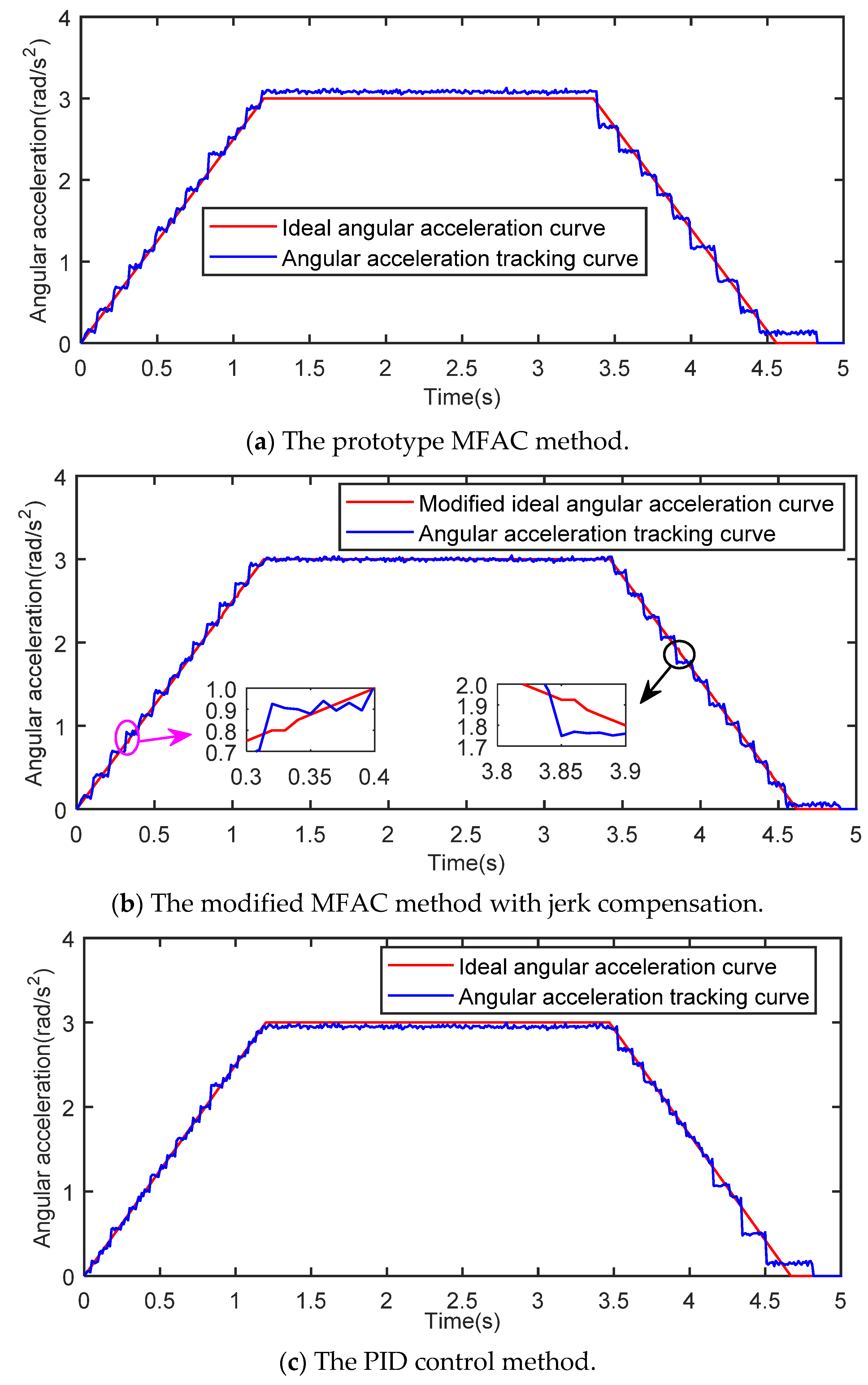
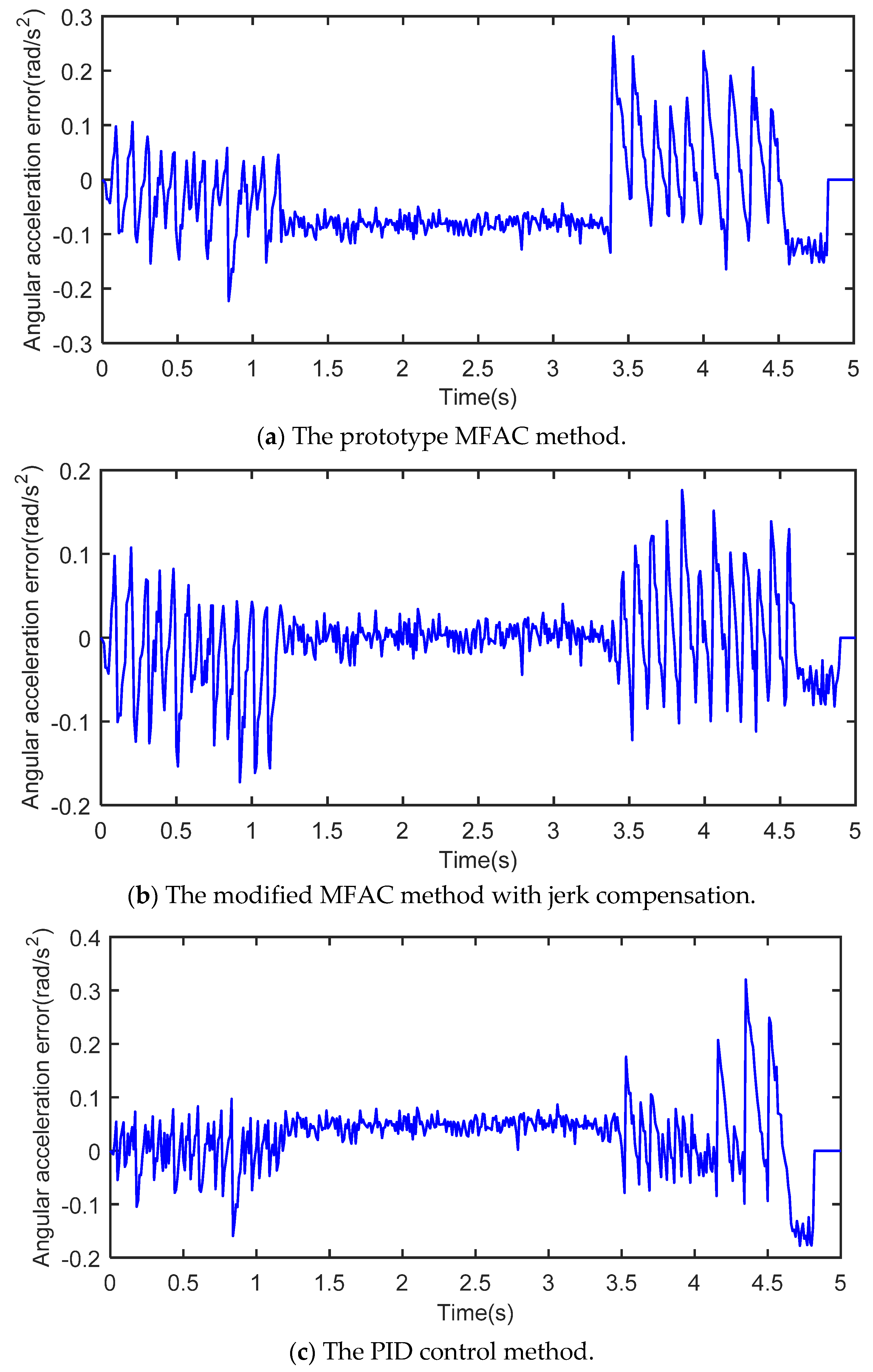
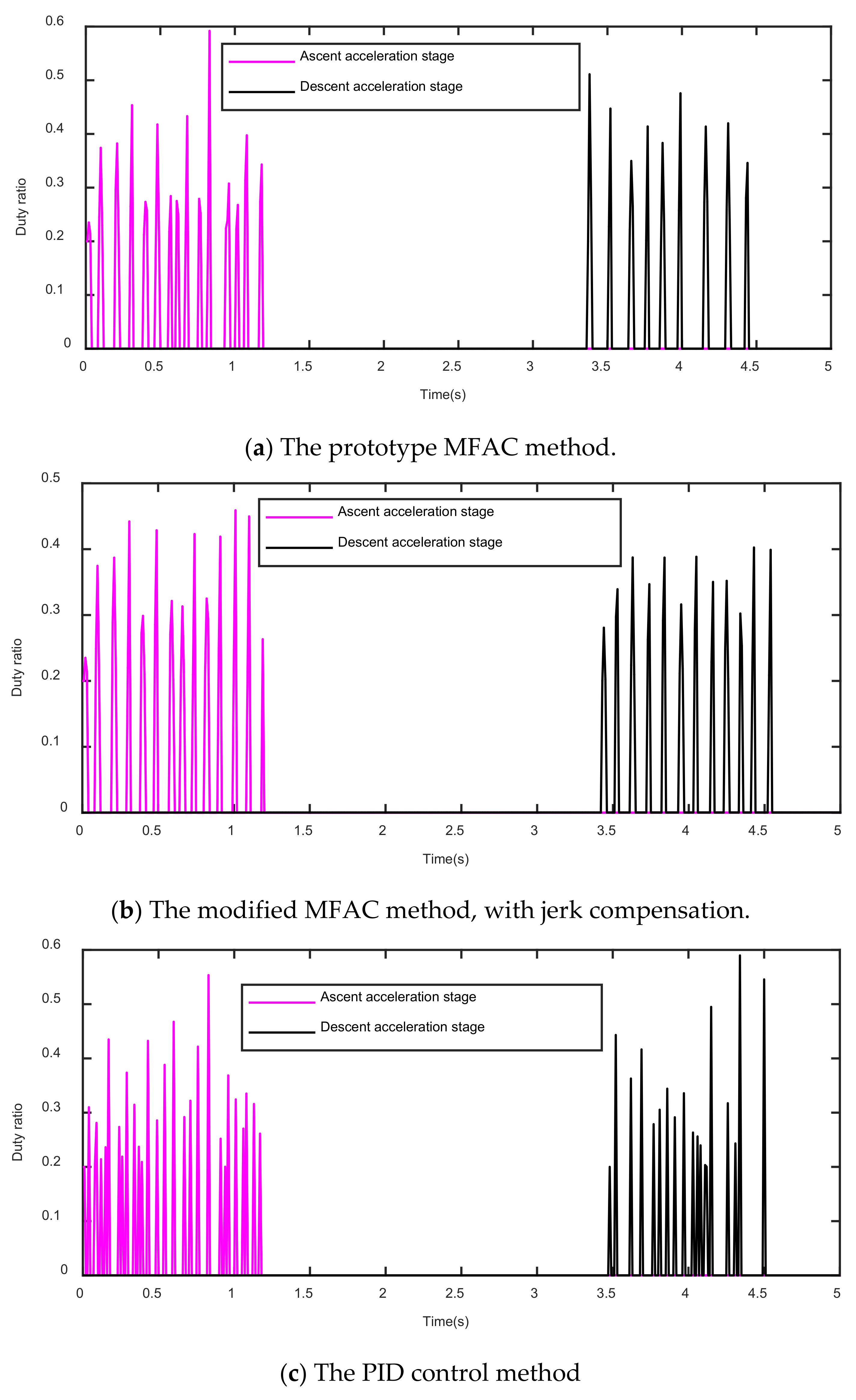
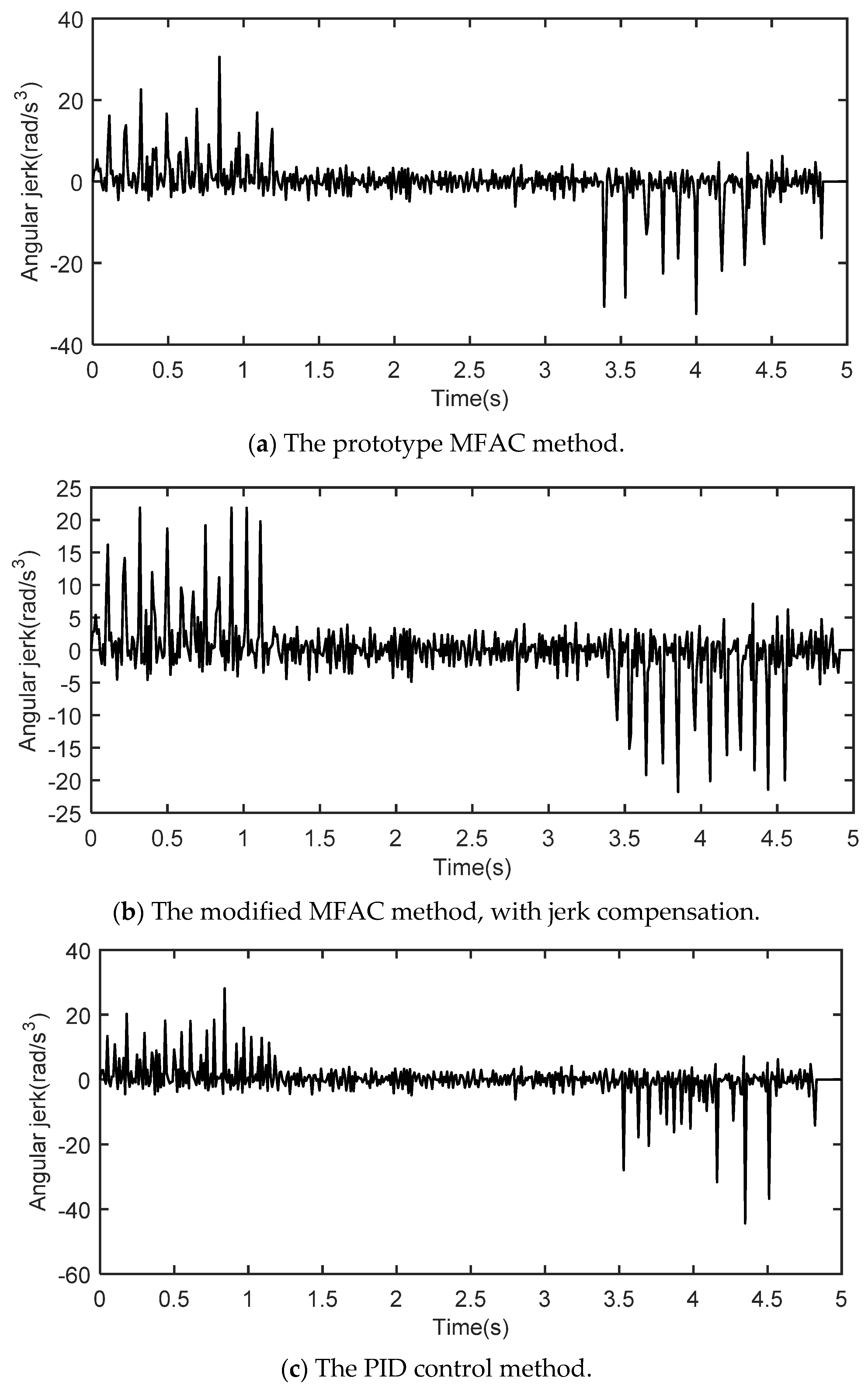
5.3. Simulation Results

The control characteristics using the modified MFAC method with jerk compensation can be discussed by comparing the prototype MFAC method and the PID control method.

According to the designed trapezoidal acceleration under the first gear position, the AMT output shaft’s ideal angular acceleration can be completed in 4.8 s. Figure 8, Figure 9, Figure 10 and Figure 11 present comparisons of tracking, comparisons of tracking error, comparisons of duty ratios, and comparisons of angular jerk curves, respectively.

In operation, the acceleration processes of the prototype MFAC method, the modified MFAC method with jerk compensation, and the PID control method were completed in 4.83 s, 4.90 s, and 4.82 s. The times of the ascent, horizontal, and descent acceleration stages using the prototype MFAC method were completed in 1.20 s, 2.16 s, and 1.47 s, respectively. The times of the ascent, horizontal and descent acceleration stages using the modified MFAC method with jerk compensation were completed in 1.20 s, 2.22 s, and 1.48 s respectively. The times of the ascent, horizontal and descent acceleration stages using the PID control method were 1.20 s, 2.27 s, and 1.35 s, respectively.

Figure 8a shows that the angular acceleration tracking curve can better track the ideal angular acceleration curve. Figure 8b shows that the angular acceleration tracking curve can track the modified ideal angular acceleration curve well, and it shows that an ideal angular acceleration curve becomes a modified ideal angular acceleration curve when the absolute of the AMT output shaft’s angular jerk is greater than 20 rad/s³. Figure 8c shows that the angular acceleration tracking curve can sensitively track the ideal angular acceleration curve.

Figure 9a shows that the absolute maximum of the AMT output shaft’s angular acceleration errors is 0.22 rad/s² during the ascent acceleration stage, which was 0.26 rad/s² during the descent acceleration stage. Figure 9b shows that the absolute maximum of the AMT output shaft’s angular acceleration error was 0.17 rad/s² during the ascent acceleration stage, which was 0.18 rad/s² during the descent acceleration stage, which is obviously less than that based on the prototype MFAC method shown in Figure 9a. Figure 9c shows that the absolute maximum of the AMT output shaft’s angular acceleration tracking error was 0.22 rad/s² during the ascent acceleration stage, and was 0.32 rad/s² during the descent acceleration stage. Obviously, the absolute maximum of the AMT output shaft’s angular acceleration error based on the modified MFAC method with jerk compensation is the least, and that based on the PID control method is the largest. Specially, the modified MFAC method with jerk compensation can clearly reduce the AMT output shaft’s angular acceleration tracking error.

Figure 10a shows that the duty ratio of the engaging solenoid valve during the ascent acceleration stage ranged from 0.20 to 0.59, and that of the disengaging solenoid valve during the descent acceleration stage ranged from 0.20 to 0.51. Figure 10b shows that the duty ratio of the engaging solenoid valve during the ascent acceleration stage was ranged from 0.2 to 0.46, and that of the disengaging solenoid valve during the descent acceleration stage ranged from 0.2 to 0.40. Figure 10c shows that the duty ratio of the engaging solenoid valve during the ascent acceleration stage changed from 0.2 to 0.55, and that of the disengaging solenoid valve during the descent acceleration stage changed from 0.2 to 0.59. Clearly, the range of the duty ratios based on the modified MFAC method with jerk compensation is less than those based on the prototype MFAC method and the PID control method. Moreover, the duty ratios of the clutch solenoid valves based on the modified MFAC method with jerk compensation changed more slowly from Figure 10b than those based on the PID control method from Figure 10c, which is advantageous for the clutch solenoid valves because changing too fast will cause shocks.

Figure 11a shows that the absolute maximum of the AMT output shaft’s angular jerk was 30.60 rad/s³ during the ascent acceleration stage, and that during the descent acceleration stage was 32.45 rad/s³. Figure 11b shows that the absolute maximum of the AMT output shaft’s angular jerk is 21.87 rad/s³ during the ascent acceleration stage, and that was 21.79 rad/s³ during the descent acceleration stage. Figure 11c shows that the absolute maximum of the AMT output shaft’s angular jerk based on the PID control method during the ascent acceleration stage was 28.11 rad/s³, and that was 44.40 rad/s³ during the descent acceleration stage. By contrast, the absolute maximum of the AMT output shaft’s angular jerk based on the modified MFAC method with jerk compensation is obviously less than that based on the prototype MFAC method and that based on the PID control method. Moreover, the absolute maximum of the AMT output shaft’s angular jerk based on the prototype MFAC method is less than that based on the PID control method, which indicates that the prototype MFAC method can control the AMT output shaft’s angular jerk better than the PID control method.

5.4. Data Analysis

The above performance parameters based on the three data-driven methods are needed to be accurately analyzed and compared.

Table 2. Data comparisons between the three data-driven methods.

Characteristic Parameter	Stage	Modified MFAC Method with Jerk Compensation	Prototype MFAC	PID
Absolute maximum of the AMT output shaft’s angular acceleration error (rad/s2)	Ascent stage	0.17	0.22	0.22
	Descent stage	0.17	0.26	0.32
Absolute maximum of the AMT output shaft’s angular jerk (rad/s3)	Ascent stage	21.87	30.60	28.11
	Descent stage	21.79	32.45	44.40

lists the main data comparisons among the three data-driven methods.

By calculation, the absolute maximum of the AMT output shaft’s angular acceleration tracking error, based on the modified MFAC method with jerk compensation, accounts for approximately 77.41% of that based on the prototype MFAC method and that based on the PID control method during the ascent acceleration stage. In addition, the absolute maximum of the angular acceleration tracking error accounts for approximately 67.09% of that based on the prototype MFAC method and approximately 55.04% of that based on the PID control method during the descent acceleration stage. Thus, the modified MFAC method with jerk compensation is a superior control method to track the ideal angular acceleration curve.

By calculation, the absolute maximum of the AMT output shaft’s angular jerk based on the modified MFAC method with jerk compensation accounts for approximately 71.16% of that based on the prototype MFAC method and approximately 77.79% of that based on the PID control method during the ascent acceleration stage. Furthermore, the absolute maximum of the AMT output shaft’s angular jerk based on the modified MFAC method with jerk compensation accounts for approximately 67.16% of that based on the prototype MFAC method and approximately 49.08% of that based on the PID method during the descent acceleration stage. Consequently, the absolute maximum of the AMT output shaft’s angular jerk based on the modified MFAC method with jerk compensation is the least, that of the AMT output shaft’s angular jerk based on the prototype MFAC method is larger, and that of the AMT output shaft’s angular jerk based on the PID control method is the largest. It is shown that modified MFAC method with jerk compensation can efficiently reduce shocks.

According to the above analysis, compared with the prototype MFAC method and the PID control method, the modified MFAC method with jerk compensation can clearly reduce the AMT output shaft’s angular jerk and has smaller angular acceleration tracking error. Thus, the modified MFAC method with jerk compensation may be a more appropriate method for controlling the AMT output shaft’s angular acceleration and angular jerk, providing better performances for AMT as a soft starter.

6. Conclusions

A new data-driven control method named the modified MFAC method with jerk compensation is studied for AMT as the soft starter in the paper. First, based on analyzing the clutch characteristics and common belt accelerations, a segmented acceleration curve, comprised of several trapezoidal acceleration curves, is proposed as the ideal acceleration curve for AMT as the soft starter. Second, the dynamic analysis of AMT is discussed. Third, based on the prototype MFAC method, the modified MFAC method with jerk compensation for controlling the AMT output shaft’s angular acceleration is given. Finally, the simulation results are analyzed by comparing the three data-driven methods—the prototype MFAC method, the modified MFAC method with jerk compensation, and the PID control method. The results prove the effectiveness of using our modified MFAC method with jerk compensation to control an AMT output shaft’s angular acceleration with less tracking error and smaller shocks.

References

1. He, D.; Liu, X.; Zhong, B. Sustainable belt conveyor operation by active speed control. Measurement 2020, 154, 107458. [Google Scholar] [CrossRef]
2. He, D.; Pang, Y.; Lodewijks, G. Green operations of belt conveyors by means of speed control. Appl. Energy 2017, 188, 330–341. [Google Scholar] [CrossRef]
3. Golovanevskiy, V.A. Kondratiev, Elastic properties of steel-cord rubber conveyor belt. Exp. Tech. 2021, 45, 217–226. [Google Scholar] [CrossRef]
4. O’Shea, J.I.; Wheeler, C.A.; Munzenberger, P.J.; Ausling, D.G. The influence of viscoelastic property measurements on the predicted rolling resistance of belt conveyors. J. Appl. Polym. Sci. 2014, 131, 40755. [Google Scholar] [CrossRef]
5. Nordell, L.K.; Ciozda, Z.P. Transient belt stresses during starting and stopping: Elastic response simulated by finite element methods. Bulk Solids Handl. 1984, 4, 93–98. [Google Scholar]
6. Xi, P.; Zhang, H.; Liu, J. Dynamics simulation of the belt conveyor possessing feedback loop during starting. J. Coal Sci. Eng. 2005, 11, 83–85. [Google Scholar]
7. Wang, G.; Zhang, L.; Sun, H.; Zhu, C. Longitudinal tear detection of conveyor belt under uneven light based on Haar-AdaBoost and Cascade algorithm. Measurement 2021, 168, 108341. [Google Scholar] [CrossRef]
8. Qiao, R.Y.T.; Pang, Y. Infrared spectrum analysis method for detection and early warning of longitudinal tear of mine. Measurement 2020, 165, 107856. [Google Scholar]
9. Ji, J.; Miao, C.; Li, X. Cosine-trapezoidal soft-starting control strategy for a belt conveyor. Math. Probl. Eng. 2019, 2019, 8164247. [Google Scholar] [CrossRef]
10. Ghayesh, M.H. Nonlinear transversal vibration and stability of an axially moving viscoelastic string supported by a partial viscoelastic guide. J. Sound Vib. 2008, 314, 757–774. [Google Scholar] [CrossRef]
11. Mallick, D.S. A tricky problem: Selection of drive systems for long-distance conveyor systems. Bulk Solids Handl. 2013, 33, 28–31. [Google Scholar]
12. Meng, Q.; Hou, Y. Effect of oil film squeezing on hydro-viscous drive speed regulating start. Tribol. Int. 2010, 43, 2134–2138. [Google Scholar]
13. Zhou, M.; Wei, C.; Yu, Y.; Zhang, Y. Oil-film clutch in soft-start of belt conveyor. J. Beijing Inst. Technol. 2002, 11, 142–145. [Google Scholar]
14. Xie, F.; Zhu, J.; Zheng, X.; Guo, X.; Wang, Y.; Agarwal, R.K. Dynamic transmission of oil film in soft-start process of HVD considering surface roughness. Ind. Lubr. Tribol. 2018, 70, 463–473. [Google Scholar] [CrossRef]
15. Cui, H.; Wang, Q.; Lian, Z.; Li, L. Theoretical model and experimental research on friction and torque characteristics of hydro-viscous drive in mixed friction stage. Chin. J. Mech. Eng. 2019, 32, 80. [Google Scholar] [CrossRef] [Green Version]
16. Wang, H.; Wang, B.; Pi, D. Two-layer structure control of an automatic mechanical transmission clutch during hill start for heavy-duty vehicles. IEEE Access 2020, 8, 49617–49628. [Google Scholar] [CrossRef]
17. Gao, B.; Lu, X.; Chen, H. Dynamics and control of gear upshift in automated manual transmissions. Int. J. Veh. Des. 2013, 63, 61–83. [Google Scholar] [CrossRef]
18. Hofman, T.; Ebbesen, S.; Guzzella, L. Topology optimization for hybrid electric vehicles with automated transmissions. IEEE Trans. Veh. Technol. 2012, 61, 2442–2451. [Google Scholar] [CrossRef] [Green Version]
19. Li, Y.; Wang, Z.; Cong, X. Constant acceleration control for AMT’s application in belt conveyor’s soft starting. Int. J. Control Autom. 2013, 6, 315–326. [Google Scholar] [CrossRef]
20. Li, Y.; Lu, Y.; Sun, H.; Yan, P. Study on load parameters estimation during AMT startup. J. Control Sci. Eng. 2018, 2018, 7391968. [Google Scholar] [CrossRef]
21. Zhao, Z.; Gu, J.; He, L. Estimation of torques transited by twin-clutch during shifting process for dry dual clutch transmission. J. Mech. Eng. 2017, 53, 77–87. [Google Scholar] [CrossRef]
22. Vasca, F.; Iannelli, L.; Senatore, A.; Reale, G. Torque transmissibility assessment for automotive dry-clutch engagement. IEEE-ASME Trans. Mechatron. 2011, 16, 564–573. [Google Scholar] [CrossRef]
23. Zhao, Z.; Wu, C.; Yang, Y.; Chen, H. Optimal robust control of shifting process for hybrid electric car with dry dual clutch transmission. J. Mech. Eng. 2016, 52, 105–117. [Google Scholar] [CrossRef]
24. He, H.; Si, T.; Sun, L.; Liu, B.; Li, Z. Linear active disturbance rejection control for three-phase voltage-source PWM rectifier. IEEE Access 2020, 8, 45050–45060. [Google Scholar] [CrossRef]
25. Pakshin, P.V.; Koposov, A.S.; Emelianova, J.P. Iterative learning control of a multiagent system under random perturbations. Autom. Remote Control 2020, 81, 483–502. [Google Scholar] [CrossRef]
26. Liu, S.; Hou, Z.; Tian, T.; Deng, Z.; Li, Z. A novel dual successive projection-based model-free adaptive control method and application to an autonomous car. IEEE Trans. Neural Netw. Learn. Syst. 2019, 30, 3444–3457. [Google Scholar] [CrossRef]
27. Hou, Z.; Xiong, S. On model-free adaptive control and its stability analysis. IEEE Trans. Autom. Control 2019, 64, 4555–4569. [Google Scholar] [CrossRef]
28. Zhu, Y.; Hou, Z. Data-driven MFAC for a class of discrete-time nonlinear systems with RBFNN. IEEE Trans. Neural Netw. Learn. Syst. 2014, 25, 1013–1020. [Google Scholar] [CrossRef]
29. Hou, Z.; Wang, Z. From model-based control to data-driven control: Survey, classification and perspective. Inf. Sci. 2013, 235, 3–35. [Google Scholar] [CrossRef]
30. Bu, X.; Hou, Z.; Zhang, H. Data-driven multiagent systems consensus tracking using model free adaptive control. IEEE Trans. Neural Netw. Learn. Syst. 2018, 29, 1514–1524. [Google Scholar] [CrossRef] [PubMed]
31. Li, D.; Hou, Z. Data-driven urban traffic model-free adaptive iterative learning control with traffic data dropout compensation. IET Control Theory Appl. 2021, 15, 1533–1544. [Google Scholar] [CrossRef]
32. Yan, Z.; Yan, F.; Liang, J.; Duan, Y. Detailed Modeling and experimental assessments of automotive dry clutch engagement. IEEE Access 2019, 7, 59100–59113. [Google Scholar] [CrossRef]
33. Li, L.; Wang, X.; Qi, X.; Li, X.; Cao, D.; Zhu, Z. Automatic clutch control based on estimation of resistance torque for AMT. IEEE-ASME Trans. Mechatron. 2016, 21, 2682–2693. [Google Scholar] [CrossRef]
34. Myklebust, A.; Eriksson, L. Modeling, observability, and estimation of thermal effects and aging on transmitted torque in a heavy duty truck with a dry clutch. IEEE-ASME Trans. Mechatron. 2015, 20, 61–72. [Google Scholar] [CrossRef]
35. Chen, Q.; Qin, D.; Ye, X. Optimal control about AMT heavy-duty truck starting clutch. Zhongguo Gonglu Xuebao/China J. Highw. Transp. 2010, 23, 116–121. [Google Scholar]
Figure 1. Diagram of the AMT soft-starting system.
Symmetry 13 01808 g001
Figure 2. Five common starting acceleration curves. 1—constant acceleration; 2—sine acceleration; 3—triangular acceleration; 4—trapezoidal acceleration; 5—parabola acceleration.
Symmetry 13 01808 g002
Figure 3. Starting acceleration curve based on AMT.
Symmetry 13 01808 g003
Figure 4. The transmission double-mass model.
Symmetry 13 01808 g004
Figure 5. Block diagram of the prototype MFAC method.
Symmetry 13 01808 g005
Figure 6. A block diagram of the MFAC method with jerk compensation.
Symmetry 13 01808 g006
Figure 7. A belt conveyor with driving power of 4 × 315 kW.
Symmetry 13 01808 g007
Figure 8. Comparisons of AMT output shaft’s angular acceleration tracking curves.
Symmetry 13 01808 g008
Figure 9. Comparisons of AMT output shaft’s angular acceleration tracking error curve.
Symmetry 13 01808 g009
Figure 10. Comparisons of duty ratio curves.
Symmetry 13 01808 g010
Figure 11. Comparisons of AMT output shaft angular jerk curves.
Symmetry 13 01808 g011