Article

Effects of Second-Order Velocity Slip and the Different Spherical Nanoparticles on Nanofluid Flow

School of Mathematics and Physics, University of Science and Technology Beijing, Beijing 100083, China
*
Author to whom correspondence should be addressed.
Symmetry 2021, 13(1), 64; https://doi.org/10.3390/sym13010064
Submission received: 12 November 2020 / Revised: 17 December 2020 / Accepted: 28 December 2020 / Published: 31 December 2020
(This article belongs to the Special Issue Integral Equations: Theories, Approximations and Applications)

Abstract

:
The paper theoretically investigates the heat transfer of nanofluids with different nanoparticles inside a parallel-plate channel. Second-order slip condition is adopted due to the microscopic roughness in the microchannels. After proper transformation, nonlinear partial differential systems are converted to ordinary differential equations with unknown constants, and then solved by homotopy analysis method. The residual plot is drawn to verify the convergence of the solution. The semi-analytical expressions between N u B and N B T are acquired. The results show that both first-order slip parameter and second-order slip parameter have positive effects on N u B of the MHD flow. The effect of second-order velocity slip on N u B is obvious, and N u B in the alumina–water nanofluid is higher than that in the titania–water nanofluid. The positive correlation between slip parameters and N d p is significant for the titania–water nanofluid.

1. Introduction

Modern industrial applications are expected to achieve higher heat transfer rates, so how to improve the heat transfer performance of heat exchanger becomes the main problem concerned by researchers. Meanwhile, microchannels have many applications such as automobile cooling systems and electronic devices in micro-sized cooling systems. Li et al. [1] and Duan et al. [2] studied the heat transfer rates of nanofluid in microchannels.
To study the flow of nanofluid, homogeneous flow models and dispersion models have been proposed. In 2006, Buongiorno [3] showed that the dispersed effects can be completely ignored due to the size of nanoparticles, and Brownian diffusion and thermophoresis are important in nanofluids. Based on the above analysis, he proposed that the homogeneous models are more appropriate for predicting the heat transfer coefficient. By using this model, Yang et al. [4] studied the variation of forced convection transport with temperature jump in continuous flow and slip flow regimes. F. Hedayati et al. [5] studied the variation of T i O 2 H 2 O nanofluid mixing convection within vertical microchannel of nanoparticle migration and asymmetric heating. R.S.Andhare et al. [6] studied pressure drop characteristics of a flat plate manifold microchannel heat exchanger. O.D. Makinde et al. [7] studied MHD variable viscosity reacting flow with thermophoresis and radiative heat transfer. A.Malvandi et al. [8] discussed effects of nanoparticle migration on alumina–water nanofluid.
Boundary conditions are critical to the model; initially, the common velocity slip is the Maxwell [9] slip condition. Kou et al. [10] studied the effects of wall slip and temperature jump on heat and mass transfer characteristics of evaporative films. A.A. Avramenko et al. [11] investigated mixed convection in a circular microchannel with the slip boundary conditions. As micro/nanotechnology develops, the size of micro/nanodevices are getting smaller and smaller. The Navier slip condition will break down at higher shear rates. In 1997, Thompson [12] developed a nonlinear slip model based on the first-order slip model proposed by Maxwell. However, many researchers found that the model could not predict the flow at a high K n number. The values calculated by the second-order slip boundary condition are closer to the experimental data. Beskok and Karniadakis [13] improved a second-order slip conditions. Based on Beskok and Karniadakis, Wu [14] improved the slip condition. Zhu et al. [15] and Almutairi et al. [16] described the effects of second-order velocity slip.
However, as a result of the migration of nanoparticles under second-order slip condition and the influence of different nanoparticles, the heat transfer of nanofluids is limited. Besides, there is little attention paid to the analytic solution [17]. In this paper, the overall goal is to study the fully developed convection of nanofluids in a parallel plate channel theoretically. Two water-based nanofluids, containing alumina and titania nanoparticles, respectively, are considered. The governing partial differential equations are transformed into ordinary differential equations with an unknown constant by using similar variables, which are solved by the homotopy analysis method (HAM).

2. Mathematical Analysis

Considering a stable, incompressible, laminar flow in a parallel-plate channel with a uniform magnetic field, the upper wall of the parallel plate channel remains insulated, while the lower wall receives a constant cooling heat flow. Taking parallel to the wall as the x-axis and perpendicular to the wall as the y-axis, a two-dimensional coordinate frame is established. Nanofluids have been studied using an improved two-component heterogeneous model. Hence, the mass, momentum, thermal energy, and nanoparticle fraction equations of the flow system can be expressed as follows:
i ( ρ U i ) = 0
t ( ρ U i ) + j ( ρ U i U j ) = i P + j μ ( i U j + j U i ) σ 0 B 0 2 U i
t ( ρ c T ) + i ( ρ c U i T ) = i ( k i T ) + ρ c ( D B i ϕ + D T T C i T ) i T + Q 0 ( T T w ) q r y
t ( ϕ ) + i ( U i ϕ ) = i ( D B i ϕ + D T T C i T )
when the nanoparticle volume fractions are different, ρ , μ , k, and c also change. The expressions are as follows:
μ ( ϕ ) = μ b f ( 1 + 39.11 ϕ + 533.9 ϕ 2 ) , A l u m i n a w a t e r μ b f ( 1 + 5.45 ϕ + 108.2 ϕ 2 ) , T i t a n i a w a t e r
k ( ϕ ) = k b f ( 1 + 7.47 ϕ ) , A l u m i n a w a t e r k b f ( 1 + 2.92 ϕ 11.99 ϕ 2 ) , T i t a n i a w a t e r
ρ = ϕ ρ p + ( 1 ϕ ) ρ b f , c = ϕ ρ p c p + ( 1 ϕ ) ρ b f c b f ρ
where p stands for particle and b f stands for base fluid. Moreover, the thermal physical properties of A l 2 O 3 nanoparticles, T i O 2 nanoparticles, and the base fluid (water) are also analyzed as follows:
c p b f = 4182 J/kgK, k b f = 0.597 W/mK, ρ b f = 998.2 kg/m 3 , μ b f = 9.93 * 10 4 kg/ms
c p A l 2 O 3 = 773 J/kgK, k A l 2 O 3 = 36 W/mK, ρ A l 2 O 3 = 3380 kg/m 3
c p T i O 2 = 385 J/kgK, k T i O 2 = 8.4 W/mK, ρ T i O 2 = 4175 kg/m 3
Based on material performance of a typical water-based nanofluid with alumina (titania/water) nanoparticles, the coefficients of Equation (3) can be calculated [3] by scale analysis. Scale analysis indicates that the heat conduction term is about 1000 times more than virtue of nanoparticle diffusion. Actually, heat transfer in connection with the diffusion of nanoparticles ρ c ( D B i ϕ + D T T C i T ) i T can be neglected in comparison with heat conduction and convection. When the flow velocity is very low, the Re is very small. Therefore, compared with viscous resistance [8], inertia effect can be ignored. Assuming hydrodynamically and thermally fully developed conditions, Equations (1)–(4) can be simplified as follows [18]:
d P d x + d d y ( μ ( ϕ ) d U d y ) σ 0 B 0 2 U = 0
y ( k ( ϕ ) T y ) + Q 0 ( T T w ) q r y = 0
y ( D B ϕ y + D T T C T y ) = 0
Radiant heat flux q r is described by Rosseland approximation [17] as follows:
q r = 4 σ * 3 δ T 4 y
Assuming that temperature difference is small enough in the flow, using Taylor series to expand T 4 , and ignoring the higher-order terms, T 4 can be expressed as a linear function [19]. The approximate expression is as follows:
T 4 4 T 3 T 3 T 4
The following appropriate transformations are:
η = y H , u = U U m , H a 2 = σ B 0 2 H 2 μ w , θ = k w ( T T w ) q w H σ = ( d p / d x ) U m / H 2 , N B T = D B D T k w T C q w H , γ = Q 0 q w H 3 k w , α = d P / d x ( μ b f u B ) / H 2
Equations (8)–(10) can be reduced to:
μ ( ϕ ) d 2 u d η 2 + d μ ( ϕ ) d η d u d η H a 2 u α = 0
k ( ϕ ) d 2 θ d η 2 + d k ( ϕ ) d η d θ d η + γ θ + 16 σ * 3 k * d 2 θ d η 2 = 0
N B T ( 1 + γ θ ) 2 ϕ η ϕ θ η = 0

3. Boundary Conditions

At micro- or nanoscale, the slip boundary condition can be used to predict accurately. In current investigations, the most common velocity slip is the Maxwell [9] slip condition. The Maxwell expression is:
u s l i p = 2 β β μ w ξ τ 3 4 N P r ( δ 1 ) δ p q
where τ = S · ( n · Π ) , q = Q · S .
Beskok and Karniadakis [13] improved the second-order slip conditions:
u s u w = 2 σ v σ v [ K n ( u n ) s + K n 2 2 ( 2 u n 2 ) s ]
where ( n ) shows gradients normal to the wall surface. Based on Beskok and Karniadakis, Wu [14] improved the slip condition in detail:
u s l i p = 2 3 ( 3 ω l 3 ω 3 2 1 l 2 K n ) λ u y 1 4 [ l 4 + 2 K n 2 ( 1 l 2 ) ] λ 2 2 u y 2 = A u y + B 2 u y 2
where l = m i n [ 1 K n , 1 ] . The expression of velocity boundary condition is as follows:
y = 0 : U = N 1 U y + N 2 2 U y 2
y = H : U = N 1 U y N 2 2 U y 2
The other boundary conditions are as follows:
y = 0 : k w T y = q w , ϕ y = D T D B 1 T C T y
y = H : T y = 0 , ϕ y = D T D B 1 T C T y
Substituting Equation (13) into Equations (20)–(23), the boundary conditions are as follows:
η = 0 : u = λ 1 u η + λ 2 2 u η 2 , θ η = 1 , θ = 0 , ϕ = ϕ w
η = 1 : u = λ 1 u η λ 2 2 u η 2
In actual applications, the mass flow rate is specified through the channels. Therefore, the average fluid velocity is introduced:
U m = 0 H U d y 0 H d y
Dimensionless variables can be obtained as follows:
0 1 u d η = 1
The average of the parameters on the cross section can be calculated using the following formula [20]:
Γ = 1 A 0 1 d A = 0 1 Γ d η
Further, θ B and ϕ B can be worked out as follows:
θ B = < ρ c u θ > < ρ c u > , ϕ B = < u ϕ > < u >
According to the bulk properties and hydraulic diameter of nanofluids, the Nusselt number can be assessed as [21]:
N u B = h H k B = 1 θ B k w k B
The non-dimensional pressure drop can be defined as:
N d p = ( d p / d x ) ( μ b f u B ) / H 2 = α
In addition, the semi-analytical relationship between N u B and N B T in the alumina–water nanofluid can be obtained as:
a 1 = 2.1494 ( 248469 551.028 N B T + 72.1567 N B T 2 0.0184761 N B T 3 )
b 1 = 68012.1 + 2498.11 N B T + 45.6722 N B T 2 1.80232 N B T 3 + 0.000305721 N B T 4
c 1 = ( 0.00184879 + 0.000522536 N B T 0.0000613978 N B T 2 + 1.57212 × 10 8 N B T 3 ) 0.0600415 + 0.0000151093 N B T × 7.47 + 1
N u B A l 2 O 3 = a 1 b 1 c 1
The semi-analytical relation between N u B and N B T in the titania–water nanofluid can be obtained as:
a 2 = 2.1494 ( 202053 426.941 N B T + 46.4139 N B T 2 0.00159493 N B T 3 )
b 2 = 20516.7 + 623.982 N B T + 7.42706 N B T 2 0.334142 N B T 3 + 7.1142 × 10 6 N B T 4
c 2 = ( 0.00148734 + 0.000369449 N B T 0.0000394933 N B T 2 + 1.35712 × 10 9 N B T 3 ) 0.0488208 + 1.73602 × 10 6 N B T × 7.47 + 1
N u B T i O 2 = a 2 b 2 c 2

4. Application of HAM

In this article, to obtain the series solutions, we adopt homotopy analysis method (HAM). HAM is one of the well-known semi-analytical methods for solving various types of linear and nonlinear differential equations (ordinary as well as partial). This method is based on coupling of the traditional perturbation method and homotopy in topology. By this method, one may obtain an exact solution or a power series solution which converges in general to the exact solution. HAM consists of the convergence control parameter, which controls the convergent region and rate of convergence of the series solution. We select the initial guess solutions:
u 0 ( η ) = 0.1 + η η 2 θ 0 ( η ) = η 2 η 2 ϕ 0 ( η ) = ϕ B
What calls for special attention is that the boundary condition (26) is not yet used, which can be used to determine the unknown parameter α k 1 . For example, when k = 1 , we are able to obtain u 1 ( η ) and its integration with η in the range [ 0 , 1 ] , which is the function of α 0 . Using the boundary condition (26), we obtain:
α 0 ( η ) = 1
In this way, u k ( η ) , θ k ( η ) , ϕ k ( η ) , α k ( η ) can be successively worked out one after another according to the order k = 0 , 1 , 2 , . . . . At mth-order, we obtain:
u ( η ) = u 0 ( η ) + k = 1 m u k ( η ) θ ( η ) = θ 0 ( η ) + k = 1 m θ k ( η ) ϕ ( η ) = ϕ 0 ( η ) + k = 1 m ϕ k ( η ) α = α 0 + k = 1 m α k
The auxiliary linear operators are:
L u = d 2 u d η 2 , L θ = d 2 θ d η 2 , L ϕ = d ϕ d η
The properties of the auxiliary linear operator are as follows:
L u [ C 1 + C 2 η + C 3 η 2 ] = 0 , L θ [ C 4 + C 5 η + C 6 η 2 ] = 0 , L ϕ [ C 7 + C 8 η ] = 0
where C i , i = 1 , . . . , 8 are constants.
Next, construct the mth-order deformation equation as follows:
L u [ u m ( η ) χ m u m 1 ( η ) ] = q h u R m ( η ) L θ [ θ m ( η ) χ m θ m 1 ( η ) ] = q h θ R m ( η ) L ϕ [ ϕ m ( η ) χ m ϕ m 1 ( η ) ] = q h ϕ ( η ) R m ( η )

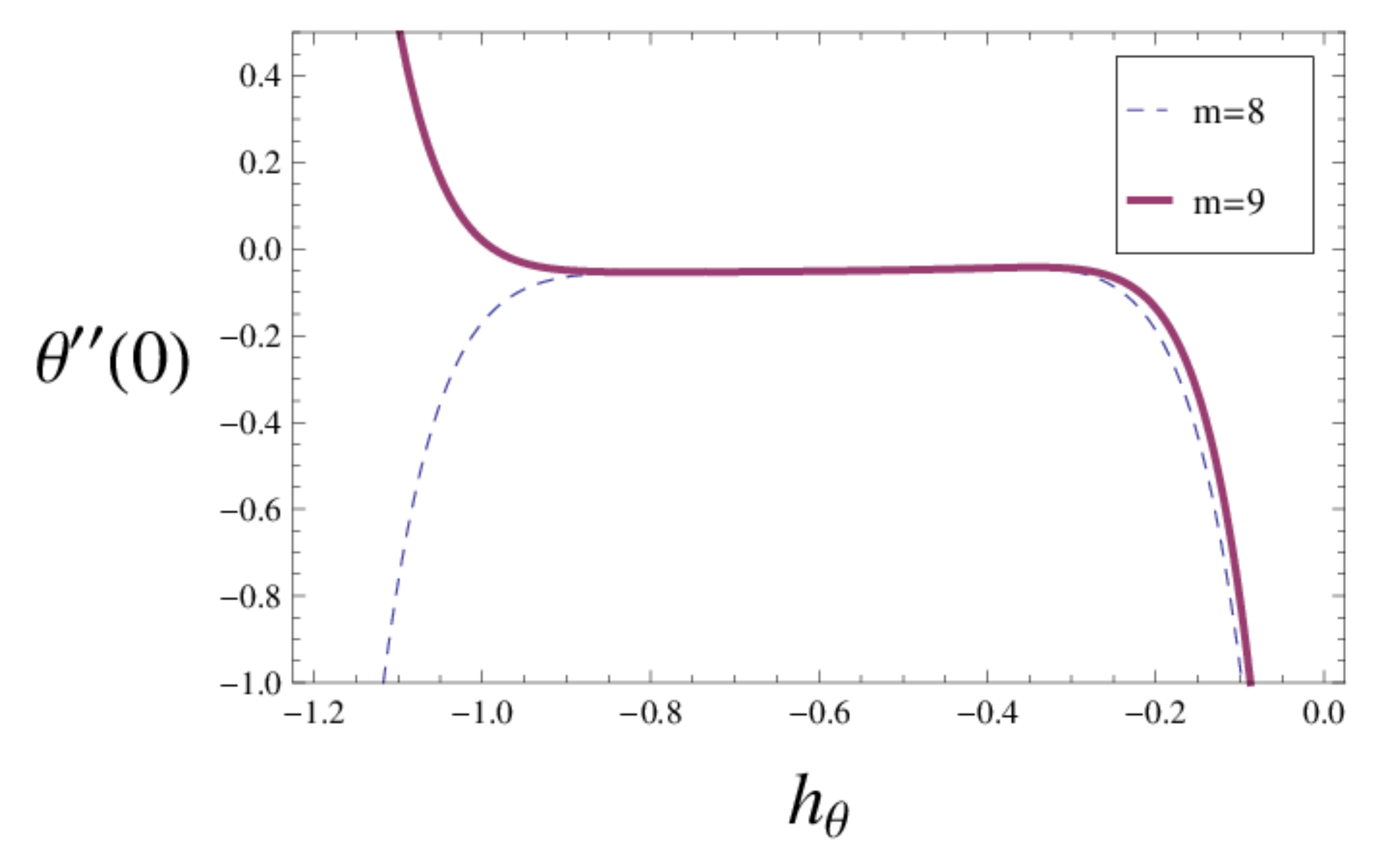
5. Convergence of the HAM Solutions

Liao [22] showed that the values of auxiliary parameters h u , h θ , and h ϕ can adjust and control the convergence of the series solutions. Directly selecting the appropriate values of h u , h θ , and h ϕ ensures the convergence of the series solutions. Figure 1 and Figure 2 give the respective valid ranges of h θ , h ϕ . The valid ranges are as follows:
0 h u 0.4 0.8 h θ 0.35 3 h ϕ 0.1
In addition, one way to find the appropriate h u , h θ , and h ϕ is to utilize the residual error. In this article, the residual error E m , t [23] is defined as follows:
E m , θ = 0 1 k θ + k θ + γ θ + 16 σ * 3 k * θ d η
Using the square residual error function, it is found that the residual error becomes more and more accurate as the order of HAM approximation increases (Figure 3). Finally, α of the HAM solution agrees well with the BVPh 2.0 solution (Table 1). BVPh 2.0 is a free software package for nonlinear boundary-value and eigenvalue problems based on HAM. In addition, it serves to show that the current results are in accordance with the results given by Yang et al. [24] (Table 2) greatly.

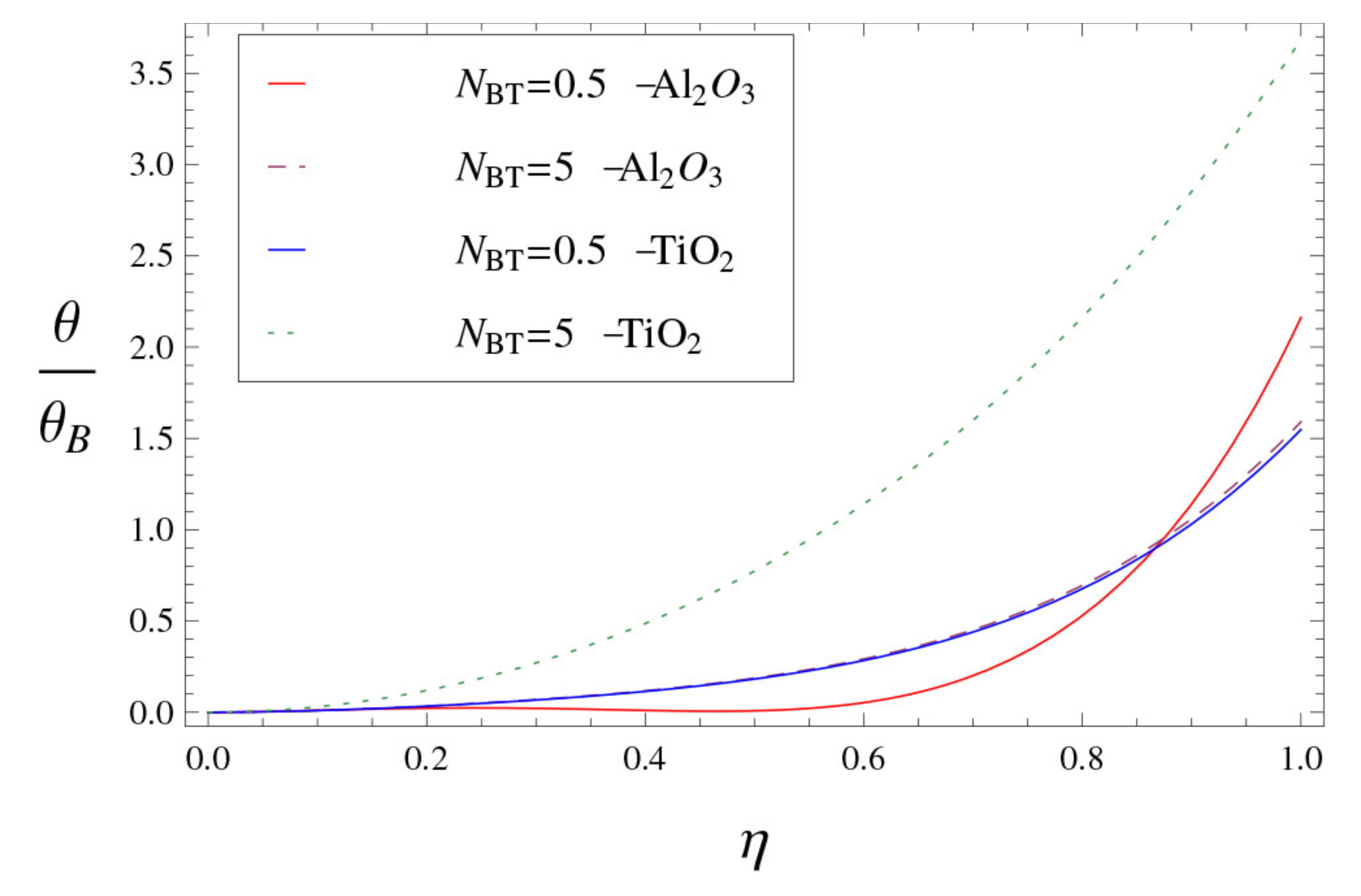
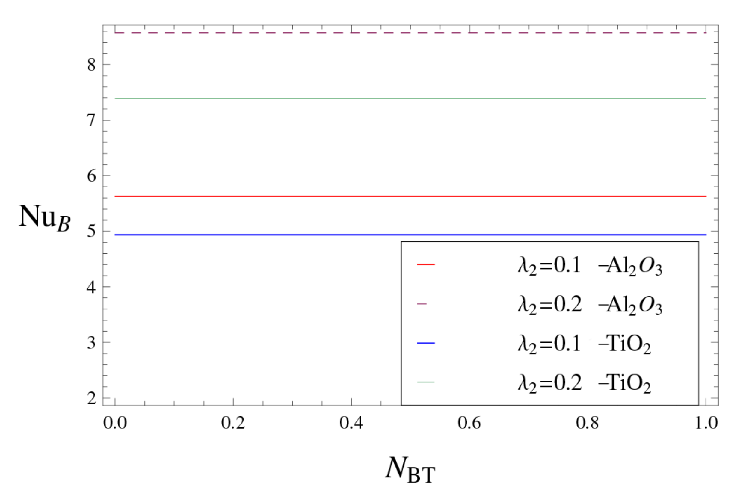
6. Results and Discussion

The effects of N B T , λ 2 and λ 1 on the nanoparticle velocity u / u B , the nanoparticle volume fraction ϕ / ϕ B , temperature profiles θ / θ B , and Nusselt number N u B are shown in Figure 4, Figure 5, Figure 6, Figure 7, Figure 8, Figure 9, Figure 10, Figure 11, Figure 12, Figure 13 and Figure 14. In these figures, η = 1 corresponds to the adiabatic wall, whereas η = 0 corresponds to the cooled wall.
The slip parameter characterizes slip resistance at the surface. The first-order velocity slip parameters λ 1 and second-order velocity slip parameters λ 2 affect the flow and heat. Figure 4, Figure 5 and Figure 6 depict the effects of second-order velocity slip λ 2 on u / u B , ϕ / ϕ B , and θ / θ B . Figure 7, Figure 8 and Figure 9 illustrate the effects of first order velocity slip λ 1 on u / u B , ϕ / ϕ B , and θ / θ B . Figure 4 and Figure 7 show that u / u B is lower near the walls and peaks near the middle of the microchannel. As Figure 4 reveals, the increase in λ 2 causes momentum to build up in the core area, with the velocity profile becoming more uniform as the slip parameters decrease. Figure 7 shows that an increase in λ 1 results in the momentum accumulation at the core region. The second-order slip condition shows a prominent effect on the velocity profile u / u B in Figure 4 and Figure 7. Assuming that mass flows are constant, in order to satisfy continuity, they must increase in the core region as the magnitude of the velocities at the boundary decreases. Meanwhile, in Figure 5 and Figure 8, the temperature profile θ / θ B decreases and then increases toward the upper wall. The titania–water nanofluid temperature changes more gently than that of the alumina–water nanofluid. The minimum of the temperature profile is increasing and shifts toward the upper wall with increasing λ 2 . Figure 8 shows no significant variation in the dimensionless temperature for λ 1 . In addition, with increasing λ 2 or λ 1 , the volume fraction ϕ / ϕ B of nanoparticles shows an increasing trend in Figure 6 and Figure 9. Hence, s more uniform distribution of the volume fraction emerges.
Figure 10, Figure 11 and Figure 12 plot the effects of N B T on u / u B , ϕ / ϕ B , and θ / θ B . Apparently, on the cooling wall, the concentration of nanoparticles is higher; at the adiabatic wall, the nanoparticle concentration is lower. Hence, the trend of the nanoparticle motion is moving from the adiabatic wall toward the cooled wall; accordingly, an uneven distribution of nanoparticles is constructed. This motion makes the viscosity near the cold wall much greater than that near the adiabatic wall, thus increasing the velocity near the adiabatic wall and decreasing the velocity near the cold wall. Therefore, the velocity profile deforms and its peak moves toward the adiabatic wall. As a result, at higher values of N B T , ϕ / ϕ B becomes more uniform, which can be observed in Figure 12. At higher value of N B T , with momentum enhanced, the heat transfer rate of the cooling wall also increases. Therefore, the increase of N B T gives rise to an increase in the temperature gradient of the cooling wall, as shown in Figure 11.
Figure 13 depicts the effect of λ 2 on the Nusselt number N u B . One thing to note is that the growth trend for N u B with the increase in λ 2 comes from the momentum accumulation near the wall. Therefore, the second-order slip parameter plays a positive role in N u B of the MHD flow. As a result, compared with Navier’s condition, under second-order slip conditions, nanofluids transfer heat more efficiently. It also must be stated that the effect of the slip parameters on N u B is quite protensive; it rests with the type of nanoparticle. In alumina–water nanofluid, the sensitivity on N u B is much higher than that of titania–water nanofluid, since the corresponding N u B of alumina–water nanofluid is higher than that of titania–water nanofluid. Figure 14 depicts the ϕ B on the N u B . It can be obtained that increasing ϕ B leads to a decrease N u B because the increasing ϕ B can increase the thermal conductivity and viscosity near walls.
Table 3 gives N d p with different λ 2 , λ 1 , N B T , and ϕ B when H a = 0, respectively. It can be concluded that both one-slip parameter and second-order slip parameter have positive correlation with the pressure drop ratio of the nanofluid to base fluid N d p . As λ 2 or λ 1 decreases, the frictional forces on the walls diminish because of the velocity jumps at the walls. However, the positive correlation is significant to titania–water nanofluid. Because of a slight increase in viscosity at the wall, N B T has a minor positive effect on N d p and ϕ B has a minor negative effect on N d p .
Table 4 gives N u B with different λ 2 , λ 1 , N B T , and ϕ B when H a = 0, respectively. It can be deduced that the velocity gradient at the wall of the microchannel increases. The slip velocity increases with the increase of velocity gradient. Thus, momentum closer to the wall increases and causes convective heat transfer to rise.

7. Conclusions

In this paper, we conduct a theoretical study on the heat transfer of alumina/water and titania/water nanofluids in a parallel-plate channel. We discuss the effects of Brownian motion and thermophoresis. Their effects are characterized by the ratio of the Brownian to thermophoretic diffusion coefficients N B T . Moreover, The second-order velocity slip condition is considered. Analytic solutions are obtained by HAM. The main conclusions of this paper can be drawn as follows:
a
The semi-analytical relation between N u B and N B T is obtained.
b
Both first-order slip parameter and second-order slip parameter have positive effects on N u B of the MHD flow, but nanofluids can transfer heat more efficiently with a second-order slip condition than with a Navier’s condition.
c
In the alumina–water nanofluid, N u B is higher than that of titania–water nanofluid.
d
The positive correlation between slip parameters and N d p is significant for the titania-water nanofluid.

Author Contributions

J.Z. conducted the original research, modified the model, and contributed analysis tools. J.C. analyzed the data, simulated the modified model, and prepared original draft. Y.L. revised the manuscript. All authors have read and agreed to the published version of the manuscript.

Funding

This research received no external funding

Institutional Review Board Statement

Not applicable.

Informed Consent Statement

Not applicable.

Data Availability Statement

Not applicable.

Acknowledgments

The work is supported by the Fundamental Research Funds for the Central Universities (FRF-BR-18-008B).

Conflicts of Interest

The authors declare that there was no conflict of interest regarding the publication of this paper.
SymbolDescription
B 0 magnetic field strength
C p specific heat (m 2 /s 2 K)
D B Brownian motion constant
D T thermophoresis diffusion coefficient
Hradius (m)
hheat transfer coefficient (W/m 2 K)
H a Hartmann number
H T C dimensionless heat transfer coefficient
kthermal conductivity (W/mK)
T free stream temperature
N B T ratio of the Brownian to
thermophoretic diffusivities
N p non-dimensional pressure drop
N u Nusselt number
ppressure (Pa)
q w surface heat flux
q r radiative heat flux
ϕ nanoparticle volume fraction
ρ density
η transverse direction
λ 1 , λ 2 slip parameters of velocity
Bbulk mean
Uaxial velocity (m/s)
Ttemperature (K)
kthermal conductivity
μ dynamic viscosity (kg/m s)
σ * Stefan–Boltzman constant
γ ratio of wall and fluid temperature
difference to absolute temperature
Subscripts
x, ycoordinate system
pnanoparticle
b f base fluid
ivelocity components

References

  1. Li, T.; Liu, B.; Zhou, J.Z.; Xi, W.X.; Huai, X.L.; Zhang, H. A Comparative Study of Cavitation Characteristics of Nano-Fluid and Deionized Water in Micro-Channels. Mathematics 2020, 11, 310. [Google Scholar] [CrossRef] [PubMed] [Green Version]
  2. Duan, Z.P.; Lv, X.; Ma, H.H.; Su, L.B.; Zhang, M.Q. Analysis of Flow Characteristics and Pressure Drop for an Impinging Plate Fin Heat Sink with Elliptic Bottom Profiles. Appl. Sci. 2020, 10, 225. [Google Scholar] [CrossRef] [Green Version]
  3. Buongiorno, J. Convective transport in nanofluids. J. Heat Transf. 2006, 128, 240–250. [Google Scholar] [CrossRef]
  4. Yang, C.; Wang, Q.L.; Nakayama, A.; Qiu, T. Effect of temperature jump on forced convective transport of nanofluids in the continuum flow and slip flow regimes. Chem. Eng. Sci. 2015, 137, 730–739. [Google Scholar] [CrossRef]
  5. Hedayati, F.; Domairry, G. Effects of nanoparticle migration and asymmetric heating on mixed convection of TiO2-H2O nanofluid inside a vertical microchannel. Powder Technol. 2015, 272, 250–259. [Google Scholar] [CrossRef]
  6. Andhare, R.S.; Shooshtari, A.; Dessiatoun, S.V.; Ohadi, M.M. Heat transfer and pressure drop characteristics of a flat plate manifold microchannel heat exchanger in counter flow configuration. Appl. Thermal Eng. 2016, 96, 178–189. [Google Scholar] [CrossRef]
  7. Ooi, E.H.; Popov, V. Numerical study of on the natural convection in Cu-water nanofluid. Int. J. Thermal Sci. 2013, 65, 178–188. [Google Scholar] [CrossRef]
  8. Ravnik, J.; Šušnjara, A.; Tibaut, J.; Poljak, D.; Cvetkovi, M. Stochastic modelling of nanofluids using the fast Boundary-Domain Integral Method. Eng. Anal. Boundary Elem. 2019, 107, 185–197. [Google Scholar] [CrossRef]
  9. Maxwell, J.C. Temperature. On Stresses in Rarefied Gases Arising from Inequalities of Temperature. Philos. Trans. R. Soc. 1879, 170, 231–256. [Google Scholar]
  10. Kou, Z.H.; Bai, M.L. Effects of wall slip and temperature jump on heat and mass transfer characteristics of an evaporating thin film. Int. Commun. Heat Mass Transf. 2011, 38, 874–878. [Google Scholar] [CrossRef]
  11. Avramenko, A.A.; Tyrinov, A.I.; Shevchuk, I.V.; Dmitrenko, N.P.; Kravchuk, A.V.; Shevchuk, V.I. Mixed convection in a vertical circular microchannel. Int. J. Therm. Sci. 2017, 121, 1–12. [Google Scholar] [CrossRef]
  12. Thompson, P.A.; Troian, S.M. A general boundary condition for liquid flowat solid surfaces. Nature 1997, 389, 360–362. [Google Scholar] [CrossRef]
  13. Beskok, A.; Karniadakis, G.E. A model for flows in channels, pipes, and ducts at micro and nano scales. Microsc. Thermophys. Eng. 1999, 3, 43–77. [Google Scholar]
  14. Wu, L.A. A slip model for rarefied gas flows at arbitrary Knudsen number. Appl. Phys. Lett. 2008, 93, 253103. [Google Scholar] [CrossRef] [Green Version]
  15. Zhu, J.; Xu, Y.X.; Hang, X. A Non-Newtonian Magnetohydrodynamics (MHD) Nanofluid Flow and Heat Transfer with Nonlinear Slip and Temperature Jump. Mathematics 2019, 7, 1199. [Google Scholar] [CrossRef] [Green Version]
  16. Almutairi, F.; Khaled, S.M.; Ebaid, A. MHD Flow of Nanofluid with Homogeneous-Heterogeneous Reactions in a Porous Medium under the influence of Second-Order Velocity. Mathematics 2019, 7, 220. [Google Scholar] [CrossRef] [Green Version]
  17. Noeiaghdam, S.; Dreglea, A.; He, J.H.; Avazzadeh, Z.; Suleman, M.; Araghi, M.A.F.; Sidorov, D.N.; Sidorov, N. Error Estimation of the Homotopy Perturbation Method to Solve Second Kind Volterra Integral Equations with Piecewise Smooth Kernels: Application of the CADNA Library. Symmetry 2020, 12, 1730. [Google Scholar] [CrossRef]
  18. Nobari, M.R.H.; Gharali, K. A numerical study of flow and heat transfer in internally finned rotating straight pipes and stationary curved pipes. Int. J. Heat Mass Transf. 2005, 49, 1185–1194. [Google Scholar] [CrossRef]
  19. Ganga, B.; Ansari, S.M.Y.; Ganesh, N.V.; Abdul Hakeem, A.K. MHD flow of Boungiorno model nanofluid over a vertical plate with internal heat generation/absorption. Propuls. Power Res. 2016, 5, 211–222. [Google Scholar] [CrossRef] [Green Version]
  20. Zhu, J.; Wang, S.N.; Zheng, L.C.; Zhang, X.X. Heat transfer of nanofluids considering nanoparticle migration and second-order slip velocity. Appl. Math. Mech. 2016, 38, 125–136. [Google Scholar] [CrossRef]
  21. Moein, S.; Mohsen, K. Study of water based nanofluid flows in annular tubes using numerical simulation and sensitivity analysis. Heat Mass Transf. 2018, 54, 2995–3014. [Google Scholar]
  22. Liao, S.J. On the homotopy analysis method for nonlinear problems. Appl. Math. Comput. 2004, 147, 499–513. [Google Scholar] [CrossRef]
  23. Fan, T. Applications of Homotopy Analysis Method in Boundary Layer Flow and Nanofluid Flow Problems. Ph.D. Thesis, Shanghai Jiao Tong University, Shanghai, China, 2012. (In Chinese). [Google Scholar]
  24. Yang, C.; Li, W.; Sano, Y.; Mochizuki, M.; Nakayama, A. On the anomalous convective heat transfer enhancement in nanofluids: A theoretical answer to the nanofluids controversy. J. Heat Transf. 2013, 135, 054504. [Google Scholar] [CrossRef]
Figure 1. h θ -curve of θ ( 0 ) .
Symmetry 13 00064 g001
Figure 2. h ϕ -curve of ϕ ( 1 ) .
Symmetry 13 00064 g002
Figure 3. The residual errors with HAM approximations order m in different nanofluids.
Symmetry 13 00064 g003
Figure 4. The effects of λ 2 on the nanoparticle velocity u / u B .
Symmetry 13 00064 g004
Figure 5. The effects of λ 2 on the temperature profiles θ / θ B .
Symmetry 13 00064 g005
Figure 6. The effects of λ 2 on the nanoparticle volume fraction ϕ / ϕ B .
Symmetry 13 00064 g006
Figure 7. The effects of first-order velocity slip parameters λ 1 on the nanoparticle velocity u / u B .
Symmetry 13 00064 g007
Figure 8. The effects of first-order velocity slip parameters λ 1 on θ / θ B .
Symmetry 13 00064 g008
Figure 9. The effects of first-order velocity slip parameters λ 1 on ϕ / ϕ B .
Symmetry 13 00064 g009
Figure 10. The effects of N B T on the nanoparticle velocity u / u B .
Symmetry 13 00064 g010
Figure 11. The effects of N B T on the temperature profiles θ / θ B .
Symmetry 13 00064 g011
Figure 12. The effects of N B T on the nanoparticle volume fraction ϕ / ϕ B .
Symmetry 13 00064 g012
Figure 13. The effects of second-order velocity slip parameters λ 2 on N u B .
Symmetry 13 00064 g013
Figure 14. The effects of ϕ B on N u B .
Symmetry 13 00064 g014
Table 1. Comparison of HAM results with BVPh2.0 results.
ϕ B α
BVPh2.0HAMRelative Error(%)
0.01−0.00286834−0.002866730.05624769
0.02−0.00396349−0.003948920.36760532
0.03−0.00527046−0.005292430.33803511
0.04−0.00678941−0.006712531.13235171
Table 2. Comparison of HAM results with those of C. Yang et al. [24].
N BT Nu B
Yang et al. [24]HAMRelative Error(%)
0.17.268237.266790.01981
0.27.558837.558890.00079
0.37.697687.694180.04547
0.47.794927.791630.04225
0.57.852277.852000.00344
0.67.900007.903380.04278
0.77.949207.945260.04956
0.87.959577.959470.00126
0.97.973137.977910.05995
18.044968.044780.00224
28.129408.129830.00529
108.218418.216300.02567
Table 3. N d p with different λ 2 , λ 1 , N B T , and ϕ B when H a = 0.
λ 2 λ 1 N BT ϕ B Types of Fluids
Al 2 O 3 -Water TiO 2 -Water
0.10.10.50.010.0001277060.000129222
0.2 0.0001319240.014154800
0.2 0.0001798800.020517000
10 0.0001277220.000127916
0.040.0001198040.000127917
Table 4. N u B with different λ 2 , λ 1 , N B T , and ϕ B when H a = 0.
λ 2 λ 1 N BT ϕ B Types of Fluids
Al 2 O 3 -Water TiO 2 -Water
0.10.10.50.015.627144.93726
0.2 8.574297.38838
0.2 8.956717.71938
10 8.693427.40811
0.048.561137.37139
Publisher’s Note: MDPI stays neutral with regard to jurisdictional claims in published maps and institutional affiliations.

