Article

The Generalized OTOC from Supersymmetric Quantum Mechanics—Study of Random Fluctuations from Eigenstate Representation of Correlation Functions

1
Centre for High Energy Physics, Indian Institute of Science, Bengaluru, Karnataka 560012, India
2
Department of Physics & Astrophysics, University of Delhi, Delhi 110007, India
3
Quantum Gravity and Unified Theory and Theoretical Cosmology Group, Max Planck Institute for Gravitational Physics (Albert Einstein Institute), Am Mühlenberg 1, 14476 Potsdam-Golm, Germany
4
National Institute of Science Education and Research, Bhubaneswar, Odisha 752050, India
5
Homi Bhabha National Institute, Training School Complex, Anushakti Nagar, Mumbai 400085, India
6
Department of Physics, Indian Institute of Technology Bombay, Powai, Mumbai 400076, India
7
Department of Chemistry, Sree Chaitanya College, Prafullanagar, Habra 743268, India
8
Department of Physical Sciences, Indian Institute of Science Education & Research Mohali, Punjab 140306, India
9
Department of Physics and Astronomy, University of Waterloo, 200 University Ave W, Waterloo, ON N2L 3G1, Canada
10
Discipline of Mathematics, Indian Institute of Technology Indore, Indore 453552, India
*
Author to whom correspondence should be addressed.
NOTE: This project is the part of the non-profit virtual international research consortium “Quantum Aspects of Space-Time & Matter” (QASTM). We would like to dedicate this work for the people those who are helping us to fight against COVID-19 pandemic across the globe.
Symmetry 2021, 13(1), 44; https://doi.org/10.3390/sym13010044
Submission received: 6 December 2020 / Revised: 15 December 2020 / Accepted: 18 December 2020 / Published: 30 December 2020
(This article belongs to the Special Issue Symmetry: Feature Papers 2020)

Abstract

:
The concept of the out-of-time-ordered correlation (OTOC) function is treated as a very strong theoretical probe of quantum randomness, using which one can study both chaotic and non-chaotic phenomena in the context of quantum statistical mechanics. In this paper, we define a general class of OTOC, which can perfectly capture quantum randomness phenomena in a better way. Further, we demonstrate an equivalent formalism of computation using a general time-independent Hamiltonian having well-defined eigenstate representation for integrable Supersymmetric quantum systems. We found that one needs to consider two new correlators apart from the usual one to have a complete quantum description. To visualize the impact of the given formalism, we consider the two well-known models, viz. Harmonic Oscillator and one-dimensional potential well within the framework of Supersymmetry. For the Harmonic Oscillator case, we obtain similar periodic time dependence but dissimilar parameter dependences compared to the results obtained from both microcanonical and canonical ensembles in quantum mechanics without Supersymmetry. On the other hand, for the One-Dimensional PotentialWell problem, we found significantly different time scales and the other parameter dependence compared to the results obtained from non-Supersymmetric quantum mechanics. Finally, to establish the consistency of the prescribed formalism in the classical limit, we demonstrate the phase space averaged version of the classical version of OTOCs from a model-independent Hamiltonian, along with the previously mentioned well-cited models.

Contents
 
1      Introduction3
 
2      Lexicography12
 
3      A Short Review of Supersymmetric Quantum Mechanics12
 
4      General Remarks on Time Disorder Averaging and Thermal OTOCs14
 
5      Eigenstate Representation of thermal OTOCs in Supersymmetric Quantum Mechanics20
5.1      Partition Function from Supersymmetric Quantum Mechanics.................................................................................................................... 23
5.2       Representation of 2-Point OTOC: Y ( 1 ) ( t 1 , t 2 ) ................................................................................................................................ 24
5.3       Representation of 2-Point OTOC: Y ( 2 ) ( t 1 , t 2 ) ................................................................................................................................ 25
5.4       Representation of 2-Point OTOC: Y ( 3 ) ( t 1 , t 2 ) ................................................................................................................................ 25
5.5       Representation of 4-Point OTOC: C ( 1 ) ( t 1 , t 2 ) ................................................................................................................................ 26
            5.5.1      Un-Normalized: C ( 1 ) ( t 1 , t 2 ) ....................................................................................................................................26
            5.5.2      Normalized: C ˜ ( 1 ) ( t 1 , t 2 ) .....................................................................................................................................27
5.6       Representation of 4-Point OTOC: C ( 2 ) ( t 1 , t 2 ) ................................................................................................................................ 28
            5.6.1       Un-Normalized: C ( 2 ) ( t 1 , t 2 ) ...................................................................................................................................28
            5.6.2       Normalized: C ˜ ( 2 ) ( t 1 , t 2 ) ....................................................................................................................................29
5.7      Representation of 4-Point OTOC: C ( 3 ) ( t 1 , t 2 ) ................................................................................................................................. 30
            5.7.1      Un-Normalized: C ( 3 ) ( t 1 , t 2 ) ....................................................................................................................................30
            5.7.2       Normalized: C ˜ ( 3 ) ( t 1 , t 2 ) ....................................................................................................................................31
5.8      Summary of Results ......................................................................................................................................................... 32
 
6      Model I: Supersymmetric Quantum Mechanical Harmonic Oscillator33
6.1       Eigenspectrum of the Super-Partner Hamiltonian............................................................................................................................. 33
6.2      Partition Function.......................................................................................................................................................... 34
6.3      Computation of 2-Point OTOCs................................................................................................................................................ 35
            6.3.1       Computation of Y ( 1 ) ( t 1 , t 2 ) ...................................................................................................................................35
            6.3.2      Computation of Y ( 2 ) ( t 1 , t 2 ) ....................................................................................................................................37
            6.3.3      Computation of Y ( 3 ) ( t 1 , t 2 ) ....................................................................................................................................38
6.4      Computation of Un-Normalized 4-Point OTOCs.................................................................................................................................. 40
            6.4.1       Computation of C ( 1 ) ( t 1 , t 2 ) ...................................................................................................................................40
            6.4.2      Computation of C ( 2 ) ( t 1 , t 2 ) ....................................................................................................................................42
            6.4.3      Computation of C ( 3 ) ( t 1 , t 2 ) ....................................................................................................................................44
6.5      Computation of Normalized 4-Point OTOCs..................................................................................................................................... 46
            6.5.1      Computation of C ˜ ( 1 ) ( t 1 , t 2 ) ..................................................................................................................................46
            6.5.2      Computation of C ˜ ( 2 ) ( t 1 , t 2 ) ..................................................................................................................................48
            6.5.3      Computation of C ˜ ( 3 ) ( t 1 , t 2 ) ..................................................................................................................................49
6.6      Summary of Results ......................................................................................................................................................... 50
 
7      Model II: Supersymmetric One-Dimensional Potential Well52
 
8      General Remarks on the Classical Limiting Interpretation of OTOCs54
 
9      Classical Limit of OTOC for Supersymmetric One-Dimensional Harmonic Oscillator55
 
10      Classical Limit of OTOC for Supersymmetric 1D Box57
 
11      Numerical Results60
11.1      Supersymmetric 1D Infinite Potential Well................................................................................................................................... 61
11.2      Supersymmetric 1D Harmonic Oscillator....................................................................................................................................... 72
 
12      Conclusions83
Appendix ADerivation of the Normalization Factors for the Supersymmetric HO86
Appendix BPoisson Bracket Relation for the Supersymmetric Partner Potential Associated with the 1D Infinite Well Potential88
Appendix CDerivation of the Eigenstate Representation of the Correlators91
Appendix C.1 Representation of 2-point Correlator: Y ( 1 ) ( t 1 , t 2 ) .................................................................................................................. 91
Appendix C.2 Representation of 2-point Correlator: Y ( 2 ) ( t 1 , t 2 ) .................................................................................................................. 92
Appendix C.3 Representation of 2-point Correlator: Y ( 3 ) ( t 1 , t 2 ) .................................................................................................................. 93
Appendix C.4 Representation of 4-Point Correlator: C ( 1 ) ( t 1 , t 2 ) .................................................................................................................. 93
            Appendix C.4.1 Un-normalized: C ( 1 ) ( t 1 , t 2 ) ....................................................................................................................................... 93
            Appendix C.4.2 Un-normalized: C ( 2 ) ( t 1 , t 2 ) ....................................................................................................................................... 95
Appendix C.5 Representation of 4-point Correlator: C ( 3 ) ( t 1 , t 2 ) .................................................................................................................. 98
Appendix C.6 Eigenstate Representation of the Normalization Factors for the 4-point Correlators...................... 100
References100

1. Introduction

The concept of out-of-time-ordered-correlators (OTOC) was first introduced by the author duo Larkin and Ovchinnikov to describe the semi-classical correlation in the context of superconductivity [1], which was mostly used in various condensed matter systems to study various out-of-equilibrium phenomena in the quantum regime [2]. However, recently, it has attracted the attention of theoretical physicists from other branches in very different contexts, finding applications in the finite-temperature extension of quantum field theories, bulk gravitational theories, quantum black holes, and many more sensational topics [3,4,5,6,7,8]. It is considered to be one of the strongest theoretical probes for quantifying quantum chaos in terms of quantum Lyapunov exponent [9], as well as quantum theories of stochasticity and randomness, among the theoretical physics community. Besides playing a key role in investigating the holographic duality [10,11,12,13] between a strongly correlated quantum system and a gravitational dual system, it also characterizes the chaotic behavior and information scrambling [14,15,16,17,18,19,20] in the context of many-body quantum systems [21,22,23]. The detailed study of OTOCs reveals an intimate relationship between three entirely different physical concepts, namely holographic duality, quantum chaos, and information scrambling. The key idea of OTOCs can be best understood as the growth of the non-commutativity of quantum mechanical operators Specifically, this non-commutative structure of the quantum operators describes the unequal time commutation relations (UETCRs) within the framework of quantum mechanics. However, the mathematical structure, as well as the physical consequences of these correlators in the quantum regime, is completely different from the concept of formulating advanced and the retarded correlators. In the later part of this paper, we will explicitly demonstrate such differences or the correlators within the framework of micro-canonical and canonical quantum statistical systems, which are defined at different time scales, and, hence, can be described using the Poisson Brackets for its classical counterpart. Not only that but also the quantum mechanical thermal ensemble average, or, equivalently, the quantum mechanical trace operation, can be described by using the phase space average in the classical limit. It is considered as the quantum mechanical analogue of the classical sensitiveness to the initial conditions in the time dynamics of a quantum system. The exponential growth of these correlators indicates the presence of chaos in the quantum system, which has led to discussions of the “butterfly effect” in black holes [24,25,26] with a saturation bound on the quantum Lyapunov exponent and for various spin models [27,28].
There has been a growing interest to understand the behavior of OTOC, even for systems where quantum chaos is expected to be absent, the most relevant example being the study of OTOC in the quantum Ising spin chain model, where power law growth of OTOCs is observed, as opposed to the exponential growth in non-integrable models in support of non-chaoticity [29,30,31]. Another interesting revelation came from a recent study of OTOCs for a quantum system with discrete energy levels, weakly coupled to a non-adiabatic dissipative thermal environment. This type of system is commonly known as open quantum system (OQS), where the OTOC was found to saturate exponentially in contrast to the exponential growth for a quantum chaotic system [32]. OTOCs have been of prime theoretical interest for diagnosing also the rate of growth of chaos with respect to the different time scales involved in the quantum system through the operators and, hence, for studying the scrambling of quantum information in black holes and strongly correlated quantum mechanical systems. It serves as a strong theoretical probe for investigating various bulk gravitational dual theories in the framework of AdS/CFT correspondence. Among others, the existence of shock waves inside black holes [33,34,35] and the maximum saturation bound of the quantum version of the Lyapunov exponent are the most famous examples where out of time ordered correlation functions have proven to be useful in the AdS/CFT correspondence. This maximum saturation bound is famously known as the Maldacena-Shenker-Stanford (MSS) bound [36]. The SYK model [37,38,39,40,41,42,43,44,45,46,47,48,49,50,51,52,53,54,55,56,57,58,59,60,61,62,63,64,65,66,67,68,69,70,71,72,73,74,75,76,77,78,79,80,81,82,83,84,85,86,87] is a well known model which saturates this well known bound and shows the signature of maximal chaos, both in its 1D CFT and gravitational dual 2D black hole counterpart. In Reference [88], this bound on quantum Lyapunov exponent was further generalized for many body systems using the well known Eigenstate Thermalization Hypothesis (ETH). Very recently, in Reference [89], the author used the tools and techniques of computing OTOC in the context of Cosmology by following the underlying slogan Cosmology meets Condensed Matter Physics to study the quantum mechanical correlation functions from random primordial fluctuations appearing in the context of cosmological perturbation theory of background spatially flat FLRW metric. Specifically, these fluctuations are appearing in the context of stochastic particle production during inflation, during the epoch of reheating, and also for the primordial phenomena, which is governed by the quantum generalization of Brownian motion, i.e., for the cosmological epochs in the time line of the universe, where the physics of out-of-equilibrium phenomena play a significant role.
In Reference [90], the earlier discussed fact regarding the exponential growth of the OTOCs in the associated time scales to describe the chaotic fluctuations for non-integrable systems has been established for various well known quantum mechanical systems. A study of the same for integrable models suggest non-chaotic quantum mechanical fluctuations in the quantum regime. In the present context, the phrase quantum randomness describes a physical phenomena which describes chaotic or non-chaotic, i.e., in principle, any random behavior of a system with respect to the associated time scales of the system. For the physical systems, such quantum randomness can be described by the following 2-fold formalisms:
  • Formalism I:
    The first approach is based on the construction and the mathematical from of the solution of the Fokker Planck equation, using which various stochastic phenomena in the quantum out-of-equilibrium regime can be studied. One of the famous examples is the stochastic cosmological particle production phenomena, which can be directly mapped to a problem of solving Schr o ¨ dinger equation with an impurity potential within the framework of quantum mechanics, which is actually describing propagation of electrons inside an electrical wire in presence of an impurity or defect. Within the framework of quantum statistical mechanics, instead of solving the Schr o ¨ dinger problem directly, or maybe solving the dynamical equation for the quantum mechanical fluctuations during the stochastic particle production, one can think about a cumulative probability distribution function of this stochastic process, P ( n , τ ) , which depends on two crucial quantities, which are: the number density of the produced particle and the associated time scale of the stochastic process. Using detailed physical arguments and computation, one can explicitly show that this probability distribution function, P ( n , τ ) , satisfies the Fokker Planck equation, which is given by:
    At infinite temperature ( β 0 ) : ̲
    1 μ P ( n , τ ) τ = n ( n + 1 ) 2 P ( n , τ ) n 2 Diffusion + ( 1 + 2 n ) P ( n , τ ) n Drift , At finite temperature ( β 0 ) : ̲ 1 μ P ( n , τ ) τ = n ( n + 1 ) 2 P ( n , τ ) n 2 Diffusion + ( 1 + 2 n ) P ( n , τ ) n Drift
    + β n ( n + 1 ) V ( n ) n P ( n , τ ) n + 2 V ( n ) n 2 P ( n , τ ) + ( 2 n + 1 ) V ( n ) n P ( n , τ ) Finite temperature contribution ,
    where μ represents the mean stochastic particle production rate and V ( n ) associated potential, which is only significant at finite temperature. By solving this set of equations in the presence of appropriate initial conditions, one can get to know about the related profile of the stochastic process semi-classically in the present context. And not only that, but one can also treat these versions of the Fokker Planck equation as the semi-classical statistical moment generating equations because, by replacing the profile function P ( n , τ ) with the appropriate moment generating function F ( n ) , one can compute all the moments. To serve this purpose, one needs to use the following fundamental equation:
    Statistical average of moment generator : F ( n ) : = d n F ( n ) P ( n , τ ) ,
    which physically represents the expectation value or the statistical average value of the number density-dependent moment generating any arbitrary function F ( n ) . Further substituting the appropriate form of this function in the moment dependent Fokker Planck equations, one can explicitly compute the expression for all the physically relevant statistical moments, i.e., n , n 2 , ⋯ explicitly without explicitly knowing about the particular mathematical structure of the profile of the related stochastic dynamical process at infinite or finite temperature for a given structure of number density potential function. These moments are extremely important in the present context of study as all of them semi-classically compute the expressions for all the equal time quantum correlation functions required to study the out-of-equilibrium aspects, such as stochastic effects, disorder, random fluctuations [91], etc., both at infinite and finite temperatures. See References [2,92,93,94,95,96], where all authors have studied the physical impact of this formalism to describe out-of-equilibrium aspects in various different contexts.
    Now, let us speak about some applicability issues related to this particular formalism. Since this formalism only allows us to know about the effect of the semi-classical correlations at equal time that might be not very interesting when we are actually thinking of doing the computation of the correlations and its rate of change at different time scales associated with the quantum mechanical system of study. For example, if we are interested in computing any general N-point semi-classical correlation function as defined by the following expression:
    i = 1 N n ( τ i ) = n ( τ 1 ) n ( τ 2 ) n ( τ N ) τ i ( i = 1 , 2 , , N ) contain disorder ,
    then this particular formalism will not work, as using this formalism one cannot capture the effect of disorder effect in the associated time scale of the system. On the other hand, by following the usual tools and techniques, one can only compute the aforementioned N-point correlators either in time ordered sense, where τ 1 > τ 2 > > τ N or in the anti-time ordered sense, where τ 1 < τ 2 < < τ N . So, from the technical ground defining this N-point correlator, including the effect of disorder in the time scale at any arbitrary temperature is also a very important topic of research, and here comes the crucial role of the next formalism where we are allowed to define and explicitly compute such quantum effects at the level of correlation functions. Another important aspect we want to point out here is that the present formalism does not bother with any Lagrangian or the Hamiltonian formulation of the associated quantum mechanical system under consideration. So, if we are really interested to know about the effect of time disordering in the expressions for the quantum mechanical correlation functions, which are defined in terms of the fundamental operators appearing in the quantum version of the Lagrangian or the Hamiltonian of the system under consideration, and also want to explicitly know about time variation with respect to different time scales associated with the system, which are actually the source of time disordering, then, instead of the present formalism, it is obviously technically correct and easier to think about the implementation of the second formalism, which gives us the better understanding of time scale disordering. In the next point, and in the rest of the paper, we will follow the second formalism to compute the quantum correlation functions from the fundamental operators from the quantum mechanical systems under study, which can explicitly capture the effect of disordering in the time scale. Not only us, but also the present trend in the research, suggests to make use of the next formalism to get better understanding of time disordering phenomena in quantum mechanical system.
  • Formalism II:
    The second approach is based on finding quantum correlation functions, including the time disordering effect, and, throughout the paper, we have followed this formalism to study effects of out-of-equilibrium physics in physical systems [89]. The present computational methodology helps us to know more about the underlying unexplored physical facts regarding the quantum mechanical aspects of various stochastic random process where time ordering or anti-time ordering is not at all important, and, instead of that, disorder in the time scale can be captured in the quantum correlations at very early time scale. This method not only helps us to know about the early time behavior of quantum correlations in the out-of-equilibrium regime of the quantum statistical mechanics but also gives crucial information regarding the late time equilibrium behavior of the quantum correlations of a specific quantum system. However, for all the systems in nature, the above interpretation of the quantum mechanical aspects of the randomness phenomena are not same. Based on all these types of quantum systems, one can categorize the random time disordering phenomena as: A.) a chaotic system which shows exponential growth in the quantum correlators, and B.) a non-chaotic system which shows periodic or aperiodic or irregular random fluctuations in the quantum correlators. The best possible theoretical measure of all such time disorder averaging phenomena for various statistical ensembles, micro-canonical and canonical ensembles, is described by out-of-time-ordered correlation (OTOC) function within the framework of quantum statistical mechanics. Let us define a set of operators, O i ( t j ) i , j = 1 , 2 with i j or i = j possibilities. The time disorder thermal average over statistical ensemble is described by the following expression: -4.6cm0cm
    C N ( i j ) ( t 1 , t 2 ) : = O i ( t 1 ) , O j ( t 2 ) N β = Tr ρ β O i ( t 1 ) , O j ( t 2 ) N i , j = 1 , 2 ,
    where the thermal density matrix ρ β is defined as:
    ρ β : = 1 Z exp β H with Z = Tr exp ( β H ) .
    In the present context, C N ( i j ) ( t 1 , t 2 ) represents three possible types of OTOC, out of which only i j possibility, which will describe only one OTOC, has been explored in earlier works in this area. The other two OTOCs appearing from the i = j possibility will be explicitly studied in this paper. The prime objective is to incorporate two more type of OTOCs, along with the well known other OTOC, to study all of the possible signatures of time disordering average from a quantum mechanical system. Our expectation is all these three types of OTOCs are able to describe the more general structure of stochastic randomness or any simple type of random process in the quantum regime. This idea was revived by Kitaev, then followed by Maldacena, Shenker, and Stanford (MSS) and many more in studying the quantum mechanical signature of chaos, which is actually the i j case in the above definition; but, the mathematical structure of the other two OTOCs represented by the i = j case suggests that any non-chaotic behavior, such as periodic or aperiodic time-dependent behavior, any time-dependent growth in the correlators which is different from any type of exponential growth, and any type of decaying behavior in the correlators, can be explained in a better way compared to just studying the time-dependent behavior from the well known OTOCs which are commonly used in the literature. So, in short, to give a complete picture of any kind of time disordering phenomena, it is better to study all these possible three types of OTOCs to finally comment on the properties of any physical systems in quantum mechanical regime. A few other important things we want to point out here for better understanding the structure of all these OTOCs capturing the underlying physics of disordering averaging phenomena: First of all, here, we have to mention that, in using the definition that we have provided in this paper, we are able to compute three sets of 2 N point OTOCs. Though, in the further computation, we have restricted our study in the paper by considering N = 1 and N = 2 cases, to study the general time disorder averaging process, one may study any even multipoint (i.e., 2 N point) correlation functions from the present definition. Now, here, the N = 1 case is basically representing a non-zero UTCR and can be treated as the building block of the full computation, as this particular case is mimicking the computation of the Green’s function in presence of time disordering. More technically, one can interpret that this contribution is made up of two disconnected time disorder averaged thermal correlator. These disconnected contributions are extremely significant if we wait for a large time scale; in literature, we usually identify this time scale as a dissipation time scale on which one can explicitly factorize any higher 2 N point correlators in terms of the non-vanishing disconnected contributions. For this specific reason, one can treat the N = 1 case result as the building block of any higher 2 N point thermal correlators. However, for most of the quantum systems, the N = 1 case shows random but decaying behavior with respect to the associated time scales which are explicitly appearing in the quantum operators of the theory. For this reason, study of any N > 1 plays a significant role to give a better understanding of the time disordering phenomena. For this purpose, next, we studied the N = 2 case, which represents the 4-point thermal correlator in the present context of study, and one of the most significant quantity in the present day research of this area, which can capture better information regarding the time disorder averaging compared to the N = 1 case. In a future version of this work, we have a plan to extend the present computation to study the physical implications of N > 2 quantum correlators to better understand the time disorder averaging phenomena. Now, we will comment on the technical side of the present formalism, using which one can explicitly compute these OTOCs in the present context. First of all, we talk about the time-independent Hamiltonians of a quantum system, which have their own eigenstates with a specific energy eigenvalue spectrum. In this case, construction of the OTOCs describing the time disorder thermal averaging over a canonical ensemble is described by two crucial components, the Boltzmann factor on which the general eigenstate dependent spectrum appears and also the temperature independent micro-canonical part of the OTOCs. At the end, we need to take the sum over all possible eigenstates, which will finally give a simplified closed expressions for OTOCs in the present context. Due to the appearance of the eigenstates from the time-independent Hamiltonian, this particular procedure will reduce the job extremely to study the time-dependent behavior of all the previously mentioned OTOCs that we have defined earlier in this paper. In the rest of the paper, we followed this prescription, which is only valid for time-independent Hamiltonian which have their own well-defined eigenstates. For more details, see the rest of the computations and related discussion that we studied in this paper. Most importantly, using this formalism, we can compute all of these OTOCs in a very simple model-independent way. The other technique is more complicated than the previously discussed one. In this case, one starts with a time-dependent Hamiltonian of the theory and uses the well-known Schwinger Keldysh formalism, which is a general path integral framework at finite temperature, for the study of the time evolution of a quantum mechanical system, which is in the out-of-equilibrium state. At the early time scale, once a small perturbation or a response is provided to a quantum system, then it is described by a out-of-equilibrium process within the framework of quantum statistical mechanics, and the present formalism provides us the sufficient tools and techniques, using which one can compute the expressions for the OTOCs. Not only that, the late time behavior of such an OTOC is described by a saturation behavior for chaotic systems, from which one can compute the various characteristic features of large time equilibrium behavior from these OTOCs.
  • Formalism III:
    The third approach is based on the circuit quantum complexity [97,98,99,100,101,102,103], which is relatively a very new concept and physically defined as the minimum number of unitary operators, commonly known as quantum gates, that are specifically required to construct the desired target quantum state from a suitable reference quantum mechanical state. In a more generalized physical prescription, quantum mechanical complexity can serve as one of several strong diagnostics for probing the time disorder averaging phenomena of a quantum mechanical system or quantum randomness. The underlying physical concept of circuit complexity can essentially provide essential information regarding various aspects of quantum mechanical randomness, such as the concept of scrambling time, Lyapunov exponent, (The associated time scale when the quantum circuit complexity starts to grow is usually identified to be the scrambling time scale and, in the representative plot with respect to the time scale, particularly, the magnitude of the slope of the linear portion of the curve is physically interpreted as the Lyapunov exponent for the specific systems where the general quantum randomness or the time disorder averaging phenomena is described by quantum chaos.), etc., which are particularly the key features of the study of quantum mechanical chaos. One can further compare between the physical outcomes of the two strongest measures of quantum randomness, which are appearing from out-of-time-order correlators (OTOCs) and the quantum mechanical circuit complexity, and comment further that, for a specific quantum system which one is capturing, there is more information regarding the description of quantum mechanical randomness.
In this paper, we generalize the study of OTOCs for investigating the phenomena of quantum randomness in various Supersymmetric integrable quantum mechanical models. The main motivation behind introducing the concept of Supersymmetry lies in the well-established fact that, for any Supersymmetric quantum mechanical model, the original Hamiltonian is always associated with a partner Hamiltonian, which, in general, is widely different from its original counterpart in terms of eigenstates. Though not always, it is possible that the quantum mechanical model under consideration attains vastly different properties in the context of quantum randomness due to the introduction of Supersymmetry within the framework of quantum mechanics. It is our expectation that this generalization of the study of all the classes of OTOCs would provide an understanding about the significant role that Supersymmetry plays in modifying the randomness behavior of the quantum mechanical models under investigation. Most importantly, from the present study, it will be clear that the additional inclusion of symmetries in the form of Supersymmetry will all affect—and, if so, then how much it will affect—the time disorder averaging phenomena for a canonical and micro-canonical statistical ensemble studied within the framework of out-of-equilibrium quantum statistical mechanics. In the eigenstate representation of the OTOCs, we actually studied three types of OTOC in this paper, out of which one of them is commonly studied in the literature, mostly used to explain the phenomena of quantum mechanical randomness (not only chaotic behavior, but also a general feature including any types of non-chaotic behavior), and the other two OTOCs that we have included in this paper might not be completely independent physical information of each other, but it is extremely important to capture the complete quantum mechanical effect in the quantum mechanical correlation functions to give a more general physical interpretation and a complete and detailed description of time disorder averaging phenomena for various quantum statistical ensembles within the framework of Supersymmetric quantum mechanics. Now, if we cannot able to find out the eigenstate representation of a given time-independent Hamiltonian within the framework of Supersymmetry, then the prescribed methodology for computing the general class of OTOCs in terms of the simplest eigenstate representation will not work. This can happen for the physical systems which are actually described by the time-dependent Hamiltonians. In that case, to compute all of these previously mentioned general classes of OTOCs, one needs to use the quantum mechanical path integral generalization of the present framework, which is commonly described by Schwinger Keldysh formalism, at finite temperature within the framework of Supersymmetric quantum mechanics. The good news is physical outcomes of such a generalization also have not been studied yet, but we have a future plan to look into at this in detail and are also hopeful that we will get a non-trivial and better understanding of various Supersymmetric quantum mechanical models out of these computations.
The mnemonic diagram shows the organization of the entire paper is appearing in Figure 1. Also the out-of-time-ordered correlation (OTOC) team is featured in Figure 2.
Organization of the paper is as follows
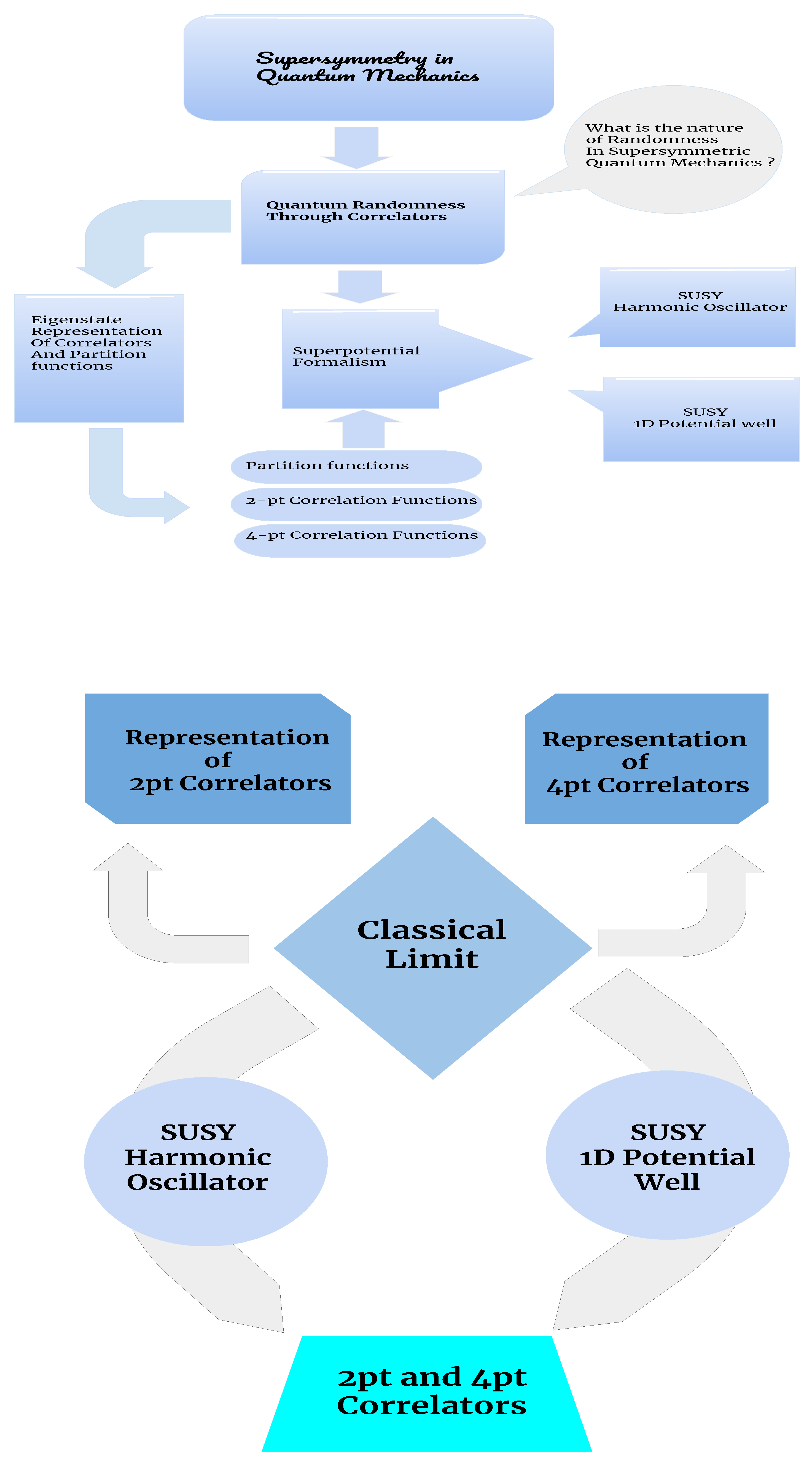
  • In Section 3, we provide a brief review of the concept of Supersymmetric Quantum Mechanics (QM).
  • In Section 4, we explain how the phenomenon of Quantum Randomness can be diagnosed through the out of time ordered correlators.
  • In Section 5, we provide a model-independent eigenstate representation of the 2- and the 4-point correlators of all the three kinds defined equally well for any QM model with well defined eigenstates.
  • In Section 6, we explicitly calculate the correlators for the Supersymmetric Harmonic Oscillator.
  • In Section 7, we provide the numerical calculations of the correlators for the Supersymmetric 1D infinite potnetial well.
  • In Section 8, we discuss the semiclassical analogue results for the two Supersymmetric QM models.
  • Finally, we conclude with the most important observations from our analysis of the considered Supersymmetric QM models.

2. Lexicography

The lexicographic notations used in this paper is appearing in the Table 1, which will be very helpful to follow various types of notations and its physical interpretations frequently used in this paper.

3. A Short Review of Supersymmetric Quantum Mechanics

The theory of Supersymmetric Quantum Mechanics [104,105,106,107,108] relates quantum eigenfunctions and the corresponding eigenvalues between two partner Hamiltonians through an intertwining relationship using the so-called charge operators. It generally uses the technique of factorizing the Hamiltonian in terms of the intertwining operators, hence determining the superpotential using the well known Riccati equation. The idea of factorizing generally allows one to express the superpotential in terms of the ground state wave-function of the original Hamiltonian of the quantum mechanical model under consideration. The process of factorization is mathematically described by the following equation:
H 1 = A A ,
where A and A are the intertwining operators which are defined from the superpotential as:
A = 1 2 d d x + W ( x ) ; A = 1 2 d d x + W ( x ) .
Within the framework of Supersymmetry, the ground state energy is usually taken to be zero, which is well justified because it is only the relative energy difference that matters. For a zero energy ground state, the Schr o ¨ dinger equation can be written as:
H 1 | Ψ 0 = 0 .
Substituting the expressions for A and A in the above equation it is not very hard to derive the Riccati equation, which further gives a way of writing the potential in terms of the superpotential given by the following expression:
V 1 ( x ) = W 2 ( x ) 1 2 W ( x ) ,
where corresponds to d / d x in the above equation. It is often an overrated fact that one needs to know the form of the potential guiding the Hamiltonian to have an idea about the wave functions of the quantum mechanical system, and the fact that the knowledge of the ground state wave function allows one to exactly know the potential associated with the system is overlooked. However, in Supersymmetric quantum mechanics, one generally utilizes this unappreciated fact to construct the potential from the known ground state wave function with zero modes:
W ( x ) = 1 2 m ψ 0 ( x ) ψ 0 ( x ) .
The knowledge of superpotential allows one to determine the Supersymmetric partner potential via the following equation:
V 2 ( x ) = W 2 ( x ) + 1 2 m W ( x ) .
The partner Hamiltonian is constructed by reversing the order of the intertwining operators used in the factorization of the original Hamiltonian. The energy eigenvalues and the eigenstates of the original and the partner Hamiltonian are not independent of each other, and that is where the beauty of Supersymmetry lies. Knowing the original Hamiltonian and its ground state, one can easily determine the energy spectrum of the partner Hamiltonian. The eigenvalues of H 1 (original Hamiltonian) and H 2 (partner Hamiltonian) are related via the following equation:
E n ( 2 ) = E n + 1 ( 1 ) ; E 0 ( 1 ) = 0 n = 0 , 1 , 2 ,
It is easy to show that the knowledge of the eigenfunctions of H 1 can be used to derive the eigenfunctions of H 2 using the A operator and the eigenfunctions of H 1 from that of H 2 using the A operator. The role of the operators A and A , apart from the conversion of an eigenfunction of the original Hamiltonian to that of its partner Hamiltonian with the same energy, also destroys or creates one node in the eigenfunction. This justifies the absence of the zero energy or the ground energy state of the partner Hamiltonian. One can put this argument simply by stating that the operator A converts an energy state of the original Hamiltonian into a lower energy state of the partner Hamiltonian keeping the energy value of the state constant. A , on the other hand, does the opposite conversion, i.e., takes an energy state of the partner Hamiltonian and converts it into an higher energy state of the original Hamiltonian, keeping the energy eigenvalue fixed.
A Supersymmetric quantum mechanical model is generally described by a Hamiltonian having the following form:
H SUSY = H 1 0 0 H 2 .
In general, for such a Hamiltonian, a quantum state is represented by:
| Ψ n T = | ψ ( 1 ) | ψ ( 2 ) ,
where, | ψ ( 1 ) and | ψ ( 2 ) are the wave functions of the original and the partner Hamiltonian, respectively.
The prime objective of this paper is to provide an eigenstate representation of the desired OTOCs that we have already defined in the introduction, using which we study the various well known quantum mechanical models in the context of Supersymmetry to study the general aspects of time disorder averaging phenomena. With this aim, one would generally look for an eigenstate of the Hamiltonian under inspection. Remembering the relation between the energy eigenvalues and eigenstates of the original and the partner Hamiltonian, it can be easily verified that the wave function given by Equation (15) is not an eigenstate of the Hamiltonian given in Equation (14). We, therefore, take the wave function of the Hamiltonian to be of the form
| Ψ n T = 1 2 | ψ ( 1 ) | ψ ( 2 ) ,
which indeed represents a normalized eigenfunction of the Hamiltonian of the Supersymmetric quantum mechanical systems considered in this work.
H SUSY | Ψ n = 1 2 H 1 0 0 H 2 | ψ n ( 1 ) | ψ n 1 ( 2 ) = 1 2 E n ( 1 ) | ψ n ( 1 ) E n 1 ( 2 ) | ψ n 1 ( 2 ) = E n ( 1 ) 2 | ψ n ( 1 ) | ψ n 1 ( 2 ) ,
where we have used the relation E n 1 ( 2 ) = E n ( 1 ) . If we use Equation (15), then | Ψ n does not remain an eigenstate of H SUSY , as we show below.
H SUSY | Ψ n = H 1 0 0 H 2 | ψ n ( 1 ) | ψ n ( 2 ) = E n ( 1 ) | ψ n ( 1 ) E n ( 2 ) | ψ n ( 2 ) .
Since the energy associated with the nth energy eigenstate of the original Hamiltonian, H 1 is not equal to that of its associated partner Hamiltonian H 2 , i.e., E n ( 1 ) E n ( 2 ) , | Ψ n fails to be an eigenstate of H SUSY .

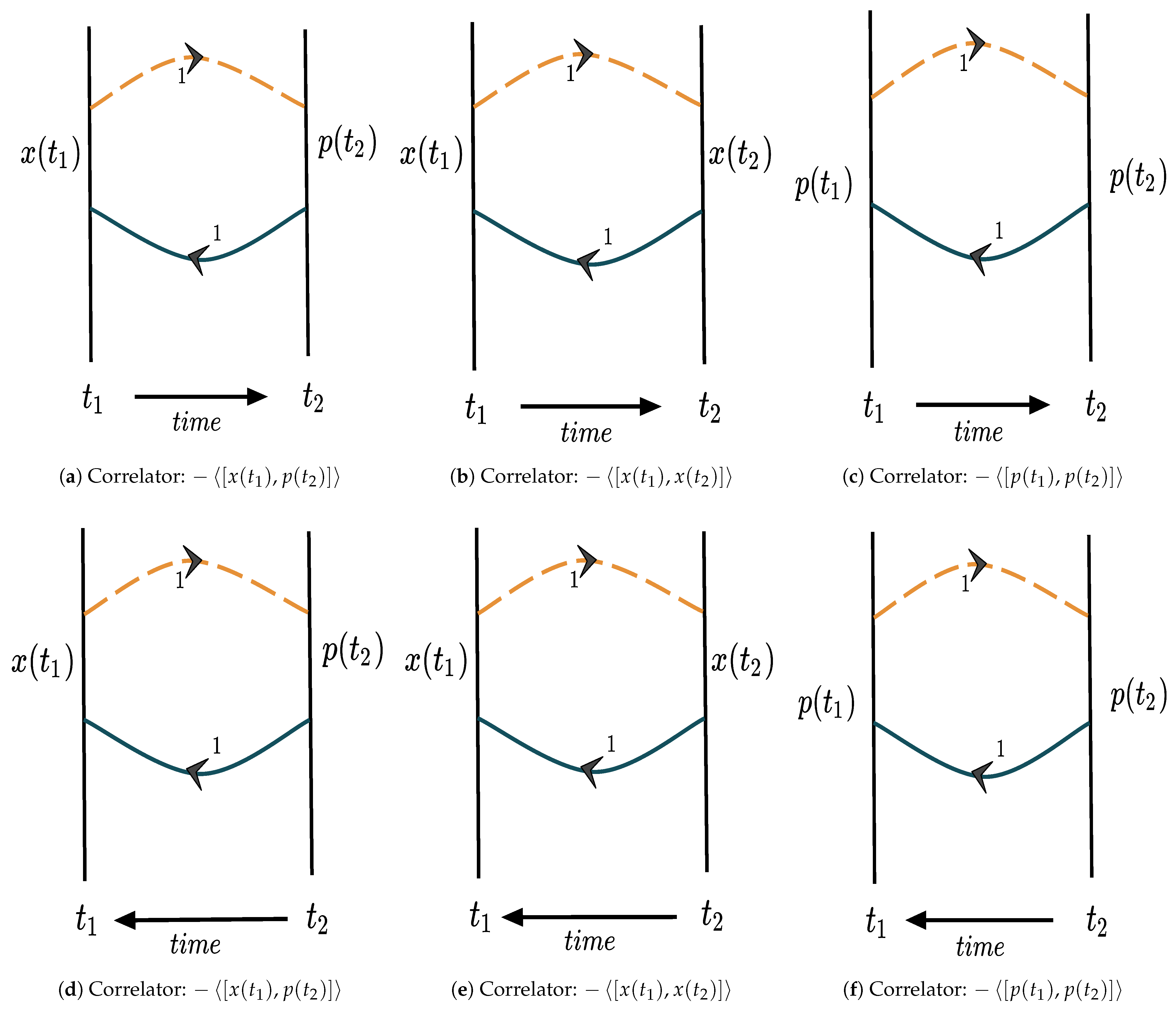
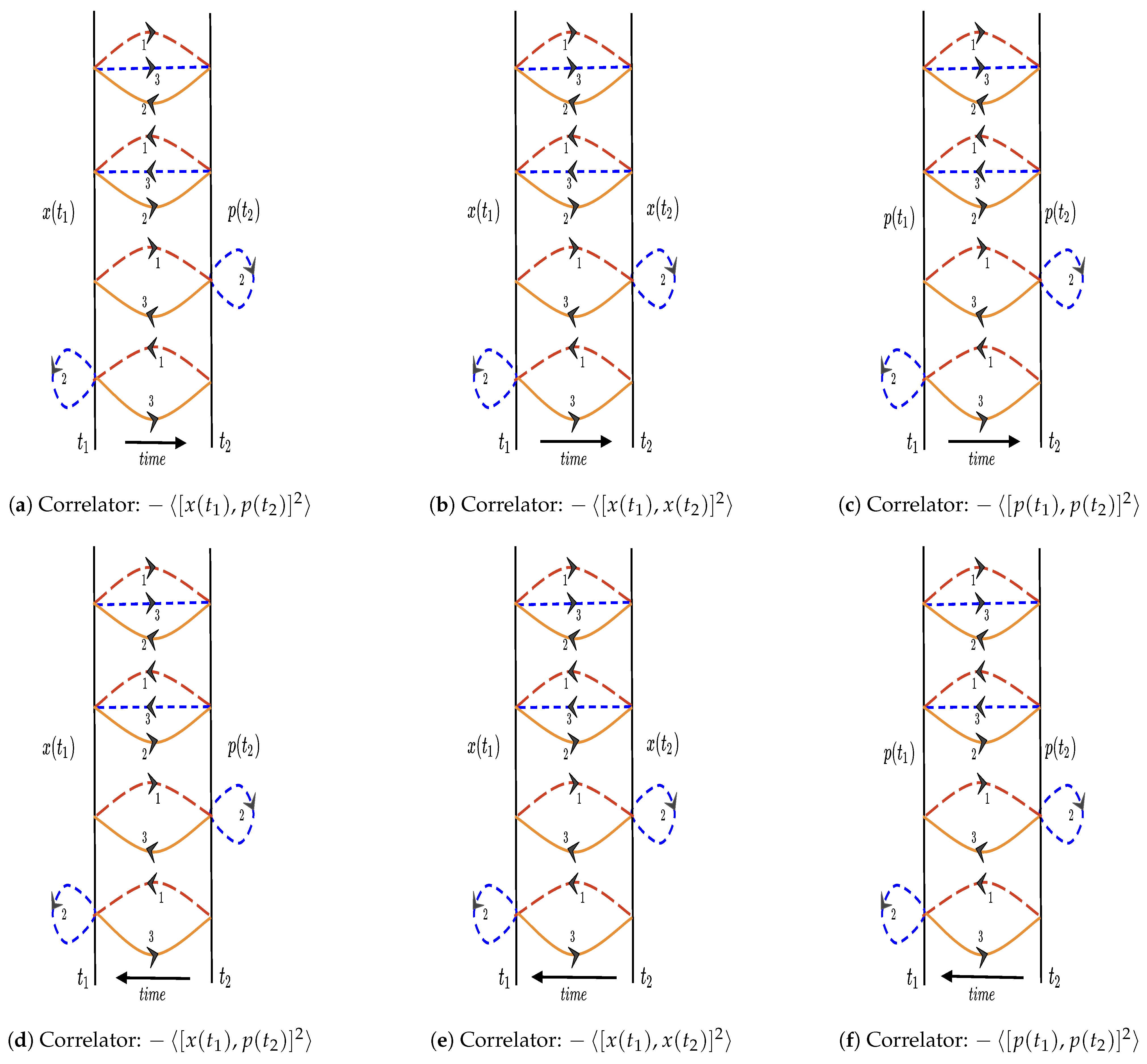
4. General Remarks on Time Disorder Averaging and Thermal OTOCs

Quantum randomness, using which we have the prime objective to technically demonstrate the time disorder averaging phenomena, is actually a very broad topic of research in theoretical physics, and there are many ways and possibilities, using which one can explicitly quantify this phenomena in the quantum regime. Quantum correlators of different orders are one of them. When a quantum state evolves to reach equilibrium at the late time scales, in that case, the overall amplitude of the correlators also evolves with the evolutionary time scales, which are usually described in terms of the fundamental quantum operators, and the time evolution of these correlators can show the presence of time disorder averaging in the form of chaotic or non-chaotic, periodic, or aperiodic random behavior in the quantum mechanical system under study. Thermal average over the canonical statistical ensemble of a quantum operator is a very powerful technique, using which one can explicitly study the time-dependent exponential growth (chaotic) or some other time-dependent non-chaotic random behavior of an operator for a quantum system that is in out of equilibrium after giving an external response. For a very long time, it was not very clear how one can actually quantify these quantum correlation functions within the framework of out-of-equilibrium quantum statistical physics. Following the previous set of works, the present work helps us to quantify, as well as to physically understand, the impact of them in the present context. In this paper, we are actually interested in three specific kinds of OTOCs, which are described by six sets of correlators, given by:
  • 2-point OTOCs: x ( t 1 ) , x ( t 2 ) , p ( t 1 ) , p ( t 2 ) , x ( t 1 ) , p ( t 2 ) ,
  • 4-point OTOCs: x ( t 1 ) , x ( t 2 ) 2 , p ( t 1 ) , p ( t 2 ) 2 , x ( t 1 ) , p ( t 2 ) 2 ,
where x is the quantum position operator, p is the associated canonically conjugate momentum, and, most importantly, both the quantum operators are defined at different time scales, which is one of the prime requirements in studying the effect of time disorder averaging phenomena through the above set of OTOCs. In addition, it is important to note that the symbol actually represents the thermal average of a time-dependent quantum operator over a canonical ensemble within the framework of quantum mechanics, which is technically defined as:
O ( t ) : = 1 Z ( t ) Tr exp ( β H ) O ( t ) = Tr ρ β O ( t ) ,
where the partition function Z and thermal density matrix operator ρ β in terms of a quantum system Hamiltonian, H, are already defined in the introduction of this paper. Since we are dealing with quantum mechanical operators, using which we are trying to understand the impact of random features in the quantum regime, it is quite expected to start with the fact that thermal 1-point function of the position operator x and momentum operator p defined at a specific time scale are zero, which can be technically demonstrated as:
x ( t ) = 0 , p ( t ) = 0 ,
where t is the associated time scale on which both of the quantum operators are evolving. For this specific reason, the explicit study and the computation of these 1-point functions are not at all important in the present context of discussion. On the other hand, due to the time translational symmetry in these thermal correlators, which is actually described by the well known Kubo Martin Schwinger condition, all the odd point OTOCs appearing in the present context will be trivially zero and, for that reason, not the object of interest in the present context of study. This can be further technically demonstrated as:
Odd x correlator : ̲ x ( t 1 ) x ( t 2 ) x ( t 3 ) odd number of terms = 0 ,
Odd p correlator : ̲ p ( t 1 ) p ( t 2 ) p ( t 3 ) odd number of terms = 0 ,
One p & even x correlator : ̲ p ( t 1 ) x ( t 2 ) x ( t 3 ) odd number of terms = 0 ,
One x & even p correlator : ̲ x ( t 1 ) p ( t 2 ) p ( t 3 ) odd number of terms = 0 .
This implies that we are only left with all even order OTOCs, out of which, in this paper, we are explicitly computing the physical outcomes from the six sets of time-dependent correlators, described by the previously mentioned 2-point and the 4-point of all possible OTOCs.
Among these correlators, two are made of different operators, which will show the perturbation of one operator measured at one time scale to the other measured at a different time, and vice versa. The other four operators are the new sets of 2- and 4-point correlators that are defined in terms of the same quantum operators, which are basically capturing the quantum effect of the self-correlation of one operator on itself having any arbitrary time-dependent profile in general to describe the phenomena of time disordering within the framework of quantum mechanics. In specific cases, it may happen that these newly defined operators show exponential growth or some other kind of growth, which is periodic or aperiodic, in the corresponding associated time scales of the quantum mechanical operator on which we are interested in the present context. In a more general context, one can see, by studying different kinds of physical systems available in the literature, where the 2-point self-correlation will decay exponentially with an associated time scale of t d , widely known as “dissipation time scale”. This particular time scale is playing the role of transition scale in the present context after reaching that the 4-point correlators can be factorized into the product of two 2-point correlation functions representing disconnected diagrams within the framework of quantum field theory. In addition, it is important to note that, here, at the “dissipation time scale”, all other terms are exponentially suppressed by the factor e t / t d , which will completely disappear from the factorized version of the 4-point correlators, on which we are interested in this paper, in the large time limit given by t t d with t . In usual prescription of the “dissipation time scale”, t d is identified with the inverse temperature β , i.e., t d β = 1 / T , where we use Boltzmann constant k B = 1 , and T physically represents the equilibrium temperature of the quantum statistical ensemble on which we are interested in. So, one can translate the large time limit in terms of the associated equilibrium temperature as t T 1 , which is not obviously true for a zero temperature case but can be justifiable in any (small or large) temperature of the system under consideration. For example, we now look into a specific 4-point thermal correlation function at the vicinity of the previously mentioned dissipation time scale, around which one can factorize it in the following specific form:
x ( t 1 ) x ( t 1 ) p ( t 2 ) p ( t 2 ) Unequal time 4 point correlator x ( t 1 ) x ( t 1 ) Equal time 2 point correlator p ( t 2 ) p ( t 2 ) Equal time 2 point correlator + O ( e t / t d ) Subdominant decaying contribution ,
where, in this aforementioned factorization, O ( e t / t d ) are the higher order correction terms, which are actually sub-dominant at the vicinity of the dissipation time scale. One more thing we can observe from the aforementioned factorization is that the individual contributions of the 2-point contributions do not mix up the time scales, and, for this reason, they can be written in terms of the product of two equal time 2-point correlators. In addition, for this particular example, when we are thinking of doing the computation with two different operators, after doing the factorization, one can easily observe that the two different operators do not mix with each other at the level of 2-point correlators. So, we are mainly interested in the terms that cannot be written in time ordered form, and those terms provide more insight to the randomness present in a system. Now, we would like to go one step further and normalize the OTOC, which is basically related to this factorization process of the 4-point correlators in terms disconnected equal time 2-point contributions. The process of normalization actually helps us to reduce the unwanted fluctuations from the computed OTOCs, which further allows us to give a clearer picture of the time-dependent behavior of the desired OTOCs in which we are interested in this paper. We do not normalize the 2-point correlation functions as they are the main building blocks of our computation of OTOCs; hence, we only normalize the 4-point OTOC as given by the following expression. We can write x ( t 1 ) , p ( t 2 ) 2 in the following simplified mathematical form:
x ( t 1 ) , p ( t 2 ) 2 = 2 x ( t 1 ) x ( t 1 ) p ( t 2 ) p ( t 2 ) Re x ( t 1 ) p ( t 2 ) x ( t 1 ) p ( t 2 ) .
After imposiing the previously mentioned constrained obtained at the vicinity of the dissipation time scale, one can further simplify the expression for the mentioned correlator as given by the following expression:
x ( t 1 ) , p ( t 2 ) 2 = 2 x ( t 1 ) x ( t 1 ) p ( t 2 ) p ( t 2 ) Re x ( t 1 ) p ( t 2 ) x ( t 1 ) p ( t 2 ) + O ( e t / t d ) .
Now, we normalize this aforementioned quantity using two different equal time 2-point correlators, which we have obtained from the factorization in terms of the disconnected pieces. Consequently, we get the following simplified form of the normalized OTOC:
C ( 1 ) ( t 1 , t 2 ) = x ( t 1 ) , p ( t 2 ) 2 x ( t 1 ) x ( t 1 ) p ( t 2 ) p ( t 2 ) = 2 1 Re x ( t 1 ) p ( t 2 ) x ( t 1 ) p ( t 2 ) x ( t 1 ) x ( t 1 ) p ( t 2 ) p ( t 2 ) .
The first expression in Equation (26) is a universal contribution, which will always appear for the quantum systems where the previously mentioned factorization process works at the vicinity of the dissipation time scale. On the other hand, the second term of Equation (26) is basically representing a normalized version of the previously mentioned 4-point function, which can only appear after dissipation time. The other two non-trivial OTOCs we are also interested in this paper are of the form x ( t 1 ) , x ( t 2 ) 2 and p ( t 1 ) , p ( t 2 ) 2 , and, by following the same logical argument at the vicinity of the dissipation time scale, we can normalize them, as well, and write them in the following simplified mathematical forms:
C ( 2 ) ( t 1 , t 2 ) = x ( t 1 ) , x ( t 2 ) 2 x ( t 1 ) x ( t 1 ) x ( t 2 ) x ( t 2 ) = 2 1 Re x ( t 1 ) x ( t 2 ) x ( t 1 ) x ( t 2 ) x ( t 1 ) x ( t 1 ) x ( t 2 ) x ( t 2 ) ,
and
C ( 3 ) ( t 1 , t 2 ) = p ( t 1 ) , p ( t 2 ) 2 p ( t 1 ) p ( t 1 ) p ( t 2 ) p ( t 2 ) = 2 1 Re p ( t 1 ) p ( t 2 ) p ( t 1 ) p ( t 2 ) p ( t 1 ) p ( t 1 ) p ( t 2 ) p ( t 2 ) .
Now, since these OTOCs acts as a theoretical probe to know about the generic chaotic or non-chaotic time-dependent behavior of quantum system, it has to satisfy the following constraints in terms of the 4-point correlations, which survived in the vicinity of the previously introduced dissipation time scale, as given by:
Re x ( t 1 ) p ( t 2 ) x ( t 1 ) p ( t 2 ) x ( t 1 ) x ( t 1 ) p ( t 2 ) p ( t 2 ) = 1 A 12 ( 1 ) e λ 1 t 1 + t 2 2 with λ 1 2 π β 1 , Chaotic 1 B 12 ( 1 ) f 1 ( t 1 , t 2 ) . Non-Chaotic
Re x ( t 1 ) p ( t 2 ) x ( t 1 ) p ( t 2 ) x ( t 1 ) x ( t 1 ) p ( t 2 ) p ( t 2 ) = 1 A 12 ( 2 ) e λ 2 t 1 + t 2 2 with λ 2 2 π β 2 , Chaotic 1 B 12 ( 2 ) f 2 ( t 1 , t 2 ) . Non-Chaotic
Re p ( t 1 ) p ( t 2 ) p ( t 1 ) p ( t 2 ) p ( t 1 ) p ( t 1 ) p ( t 2 ) p ( t 2 ) = 1 A 12 ( 3 ) e λ 3 t 1 + t 2 2 with λ 3 2 π β 3 , Chaotic 1 B 12 ( 3 ) f 3 ( t 1 , t 2 ) . Non-Chaotic
The aforementioned expression captures all the possibilities which one can observe in different quantum mechanical systems available in nature. Here, A 12 ( 1 ) , A 12 ( 2 ) , and A 12 ( 3 ) are the quantum mechanical model-dependent pre-factors which show exponential growth (chaotic behavior) in the 4-point correlator with respect to the time scales associated with the system under study. On the other hand, B 12 ( 1 ) , B 12 ( 2 ) , and B 12 ( 3 ) are the quantum mechanical model-dependent pre-factors which show any type of time-dependent fluctuations (non-chaotic behavior). In addition, for the general prescription, the quantum Lyapunov exponents, λ 1 , λ 2 , and λ 3 , are not the same for which the MSS bound on quantum chaos from these three cases are also not the same. Consequently, the equilibrium saturation temperatures at the late time scales from these three OTOCs also differ from each other, i.e., β 1 β 2 β 3 . In addition, it is important to point out that the mathematical structure of the time-dependent functions f 1 ( t 1 , t 2 ) , f 2 ( t 1 , t 2 ) , and f 3 ( t 1 , t 2 ) are also different for general quantum mechanical set ups. When we are considering the quantum mechanical models described by time-dependent Hamiltonians, in that case, these expectations and all sorts of predictions work very well. However, when we are thinking about particularly quantum mechanical models which are described by the time-independent Hamiltonian and the eigenstate representation of OTOCs, in that situation, one might have further simplifications. There might be a possibility to have an underlying connection between the two functions f 2 ( t 1 , t 2 ) and f 3 ( t 1 , t 2 ) in the eigenstate representation of the OTOCs in the non-chaotic case, and, for this reason, they might not be capturing completely independent information of the time disorder averaging. On the other hand, in the chaotic case, if three of the OTOCs independently show exponential growth in the time scale, the quantum Lyapunov exponents and the related equilibrium saturation temperatures are not at all same, even in the eigenstate representation. But, if the first OTOC is showing the chaotic behavior, and other two are not, in that case, the previous connection between the two functions f 2 ( t 1 , t 2 ) and f 3 ( t 1 , t 2 ) holds good in the eigenstate representation.
In Figure 3 and Figure 4, we present the diagrammatic representations of all types of OTOCs in which we are interested in this paper. Particularly, in Figure 3, we explicitly depict the possible 2-point OTOCs. Here, we have three possibilities, which are given by [ x ( t 1 ) , p ( t 2 ) ] , [ x ( t 1 ) , x ( t 2 ) ] , and [ p ( t 1 ) , p ( t 2 ) ] . Since each OTOC is made up of a commutator bracket in the quantum mechanical description, for each case, we have two different contributions having overall opposite signatures. Further, to draw the representative diagrams, we need to consider the flow of time scale from t 1 to t 2 or t 2 to t 1 . In all the representative diagrams, the two vertical solid thick lines correspond to the specific time slice having time t = t 1 and t = t 2 , respectively. It is understandable, from the mathematical structure of the mentioned 2-point OTOCs, that, since the correlator involves only two time scales, that is why drawing two vertical parallel lines are physically justifiable in the present context. Because of the previously mentioned flow of time scale from t 1 to t 2 or t 2 to t 1 for each 2-point OTOCs, we have two possible diagrams. So, as a whole, for the 2-point OTOCs, one can draw six possibilities. In addition, by studying each of the diagrammatic representations, we can also observe that each of the contributions of the 2-point functions are represented by separate lines with representative arrows which completely depend on the structure of the individual 2-point correlators. To differentiate between these two contributions, we have used red dotted line and blue solid line in the representative diagrams. Further, in Figure 4, we have explicitly shown the possible 4-point OTOCs in the present context of discussion. Here, we can draw three possible representative diagrams, which are coming from the three possible OTOCs, as given by, [ x ( t 1 ) , p ( t 2 ) ] 2 , [ x ( t 1 ) , x ( t 2 ) ] 2 , and [ p ( t 1 ) , p ( t 2 ) ] 2 . Here, as we can see that each of the OTOCs is made up of commutator bracket squared contributions in the quantum description, for each case, we have four contributions if we expand them. Out of these four 4-point thermal correlators, two of them have a positive signature, and other two have an overall negative signature in the front of each contribution. Just like the 2-point OTOCs, here, we also need to consider the flow of time scale from t 1 to t 2 or from t 2 to t 1 . It is understandable, from the mathematical structure of the mentioned 4-point OTOCs, that, because the correlator involves only two time scales instead of four different time scales, is why drawing two vertical parallel lines to represent the time slice at t = t 1 and t = t 2 are physically justifiable in the present context. Now, because of the time scale flow, each of the 4-point OTOCs have two contributions in the diagrammatic representation. In addition, for a given time flow, we have four possible diagrams, which we show in a single diagram, for the sake of simplicity. So, as a whole, to consider both the possibilities of the time flow, we have cumulatively 24 diagrams from the 4-point OTOCs. Like the previous case, here, to differentiate between each of the individual terms for a given OTOC with a specified time flow, we have also used a red dotted line, blue dotted line, and red thick line, respectively, in the representative diagrammatic representations. Last but not least, here, it is important to point that these set of diagrams are the simplest version of the well known Feynman diagrams as appearing in the context of quantum field theory literature. However, within the present framework, we do not have exactly similar Feynman diagrams, but, to understand the structure of the previously mentioned OTOCs, the present version of the diagrammatic representations play a very crucial role. All of the arrows appearing in all the diagrams represent an underlying time disordering upon which we have to take the final average in the present context.

5. Eigenstate Representation of thermal OTOCs in Supersymmetric Quantum Mechanics

In this section, our prime objective is to study various thermal correlators, OTOCs, and see how they can be expressed in a model-independent manner in the framework of quantum mechanics. We also demarcate clearly the effect of Supersymmetry and how it modifies the functional form of the correlators at the end.
To perform this explicit computation, we will follow the prescription outlined in Reference [90] to compute all the thermal OTOCs we have mentioned in the previous section of this paper (Reference [90], particularly, is extremely important for our computation because, here, the authors first have performed the computation of the first OTOC, [ x ( t 1 ) , p ( 0 ) ] 2 (though, in our computation, we have generalized this to [ x ( t 1 ) , p ( t 2 ) ] 2 ) in the eigenstate formalism for a time-independent quantum mechanical model-independent Hamiltonian.). According to this prescription, for any time-independent Hamiltonian, we define the expectation value of quantum mechanical operators as thermal expectation value in the present context, which one can easily apply for a canonical quantum statistical ensemble. Let us say a quantum mechanical time-dependent operator A ( t ) is defined on a specific Hilbert Space H with an associated Hamiltonian H (which is time-independent, obviously) and the eigenvalues (eigen energy spectrum) of H corresponding to a infinite tower of eigenkets | Ψ n n = 0 , 1 , , , where the corresponding energy levels are characterized by the index n. This energy eigenspectrum is represented by E n n = 0 , 1 , , . Then, for a canonical quantum statistical ensemble, the thermal expectation value of the quantum mechanical time-dependent operator A ( t ) at inverse temperature β , considering the Boltzmann constant k B = 1 , is defined as:
A ( t ) β = 1 Z Tr e β H A ( t ) ,
where the thermal partition function is represented by Z such that Z = Tr e β H . Here, our job is to represent this mathematical trace operation in terms of the sum over all possible eigenstates starting from the ground state ( n = 0 ). Once we are able to express this operation clearly, then the rest of the story is very typical, and, following this, one can easily compute all of the mentioned OTOCs in the eigenstate representation. It pays to use the thermal representation for expectation values of quantum mechanical operators because there are many physical models and physically relevant toy models which have well-studied structure of time-independent Hamiltonians; hence, we can utilize this property to give an eigenstate representation to the correlators as presented elaborately in this work. Consequently, the analysis presented in this paper is physically justifiable, applicable, and believable, as such, to quantum mechanical models with a well-defined Hamiltonian. In the eigenstate representation, the thermal expectation value of a quantum mechanical time-dependent operator A ( t ) can be written as:
A ( t ) β = 1 Z Tr e β H A ( t ) n | Ψ n Ψ n | Identity operator = n e β E n Ψ n | A ( t ) | Ψ n n e β E n .
Here, we work in the Heisenberg Picture, where the operators evolve with time, as given by O H ( t ) = e i H t O S ( 0 ) e i H t , where O H ( t ) represents operator O H at time scale t in Heisenberg picture and O S ( 0 ) represents its Schr o ¨ dinger picture representation at all time scales since operators do not evolve with time in Schr o ¨ dinger picture. The latter is denoted as O S to simplify the notation and make it easier to read.
What do we learn here?:
Thermal Expectation Value : A ( t ) β = 1 Z Tr e β H A ( t )
Heisenberg Repsentation of Operators : O H ( t ) = e i H t O S e i H t
Eigenstate Rep . of Thermal Exp . : A ( t ) β = n e β E n Ψ n | A ( t ) | Ψ n n e β E n
To demonstrate the computation further, let us consider a general time-independent Hamiltonian of the following form:
H ( q i , p i ) = i = 1 N p i 2 + V ( q i ) ,
where we have used the fact that the mass of all N number of particles are the same and given by m i = m = 1 / 2 to make the further computation simpler. Now, here, it is very easy to prove the following relation (see Reference [90]), which relates the quantum mechanical momentum operator matrix elements with that of the position and the energy operator matrix elements by the following expression:
p k m = i 2 E k m x k m .
Furthermore, the role Supersymmetry plays in modification of non-Supersymmetric quantum mechanical observables can be seen vis-a-vis the matrix elements of observables. Let us consider a simple matrix element for the position operator x. In the following chart, we show exactly how the matrix elements in non-Supersymmetric quantum mechanical theories and Supersymmetric quantum mechanical theories are connected:
x m k = Ψ m | x | Ψ k = 1 2 ψ m B | x | ψ k B bosonic part non SUSY & SUSY + ψ m 1 F | x | ψ k 1 F fermionic part SUSY only neither m / k is ground state SUSY switch off ψ m B | x | ψ k B , if one of m / k is ground state SUSY 1 2 ψ m B | x | ψ k B , both m & k are ground state SUSY ψ m B | x | ψ k B .
The modifications due to Supersymmetry can clearly be traced back to the fact that we could formulate a wave function of total Hamiltonian as given in Equation (16) from the two partner Hamiltonians H 1 and H 2 , as appearing from the bosonic and the fermion sectors in Supersymmetry. In fact, it is the factorization property of H 1 and H 2 which generalizes to a more powerful setting in terms of Supersymmetric generalized description of the theory under consideration. One might consider the power of the Supersymmetric description in two ways:
  • First, one can merely consider it as a tool to solve non-trivial potentials by means of solutions of their partner ones, provided that the partner ones are easily solvable.
  • Secondly, one can consider it as a more unifying description of a more beautiful theory based on the principles of symmetries of nature. It is this second philosophy which has been considered in this work.
We will consider the following six correlators in this work as stated below:
Correlation Functions
2 - point Correlator : Y ( 1 ) ( t 1 , t 2 ) = [ x ( t 1 ) , p ( t 2 ) ] β
2 - point Correlator : Y ( 2 ) ( t 1 , t 2 ) = [ x ( t 1 ) , x ( t 2 ) ] β
2 - point Correlator : Y ( 3 ) ( t 1 , t 2 ) = [ p ( t 1 ) , p ( t 2 ) ] β
4 - point Correlator : C ( 1 ) ( t 1 , t 2 ) = [ x ( t 1 ) , p ( t 2 ) ] 2 β
4 - point Correlator : C ( 2 ) ( t 1 , t 2 ) = [ x ( t 1 ) , x ( t 2 ) ] 2 β
4 - point Correlator : C ( 3 ) ( t 1 , t 2 ) = [ p ( t 1 ) , p ( t 2 ) ] 2 β
We will also consider normalized 4-point Correlation Functions, and the discussion pertaining to those is provided in the previous section:
Normalized 4-point Correlation Functions
Normalized 4 - point Correlator : C ˜ ( 1 ) ( t 1 , t 2 ) = C ( 1 ) ( t 1 , t 2 ) x ( t 1 ) x ( t 1 ) β p ( t 2 ) p ( t 2 ) β = [ x ( t 1 ) , p ( t 2 ) ] 2 β x ( t 1 ) x ( t 1 ) β p ( t 2 ) p ( t 2 ) β
Normalized 4 - point Correlator : C ˜ ( 2 ) ( t 1 , t 2 ) = C ( 2 ) ( t 1 , t 2 ) x ( t 1 ) x ( t 1 ) β x ( t 2 ) x ( t 2 ) β = [ x ( t 1 ) , x ( t 2 ) ] 2 β x ( t 1 ) x ( t 1 ) β x ( t 2 ) x ( t 2 ) β
Normalized 4 - point Correlator : C ˜ ( 3 ) ( t 1 , t 2 ) = C ( 3 ) ( t 1 , t 2 ) p ( t 1 ) p ( t 1 ) β p ( t 2 ) p ( t 2 ) β = [ p ( t 1 ) , p ( t 2 ) ] 2 β p ( t 1 ) p ( t 1 ) β p ( t 2 ) p ( t 2 ) β

5.1. Partition Function from Supersymmetric Quantum Mechanics

In the context of Supersymmetric quantum mechanics, the partition function, Z, can be can be expressed in terms of the eigenstate by the following expression:
Z = Tr [ e β H SUSY ] = m Ψ m | e β H SUSY | Ψ m .
Here, the underlying relation between Supersymmetric total system and the component (or partner) systems, as discussed in Section 3, is established through the following relations:
H SUSY = H 1 0 0 H 2 e β H SUSY = e β H 1 0 0 e β H 2 , | Ψ m T = 1 2 | ψ m ( 1 ) | ψ m 1 ( 2 ) ; | Ψ 0 T = | ψ m ( 1 ) 0 .
So, the Supersymmetric quantum partition function in the eigenstate representation can be explicitly written as:
Z = ψ m ( 1 ) | e β H 1 | ψ m ( 1 ) | m = 0 + 1 2 m > 0 ψ m ( 1 ) | e β H 1 | ψ m ( 1 ) + ψ m 1 ( 2 ) | e β H 2 | ψ m 1 ( 2 ) , = e β E m ( 1 ) ψ m ( 1 ) | ψ m ( 1 ) | m = 0 Ground State Contribution + 1 2 m > 0 e β E m ( 1 ) ψ m ( 1 ) | ψ m ( 1 ) + e β E m 1 ( 2 ) ψ m 1 ( 2 ) | ψ m 1 ( 2 ) .
As shown in Section 3, in Supersymmetric quantum mechanical theories, we have the following constraint:
E m = E m ( 1 ) = E m 1 ( 2 ) ,
with the requirement that the ground state is eigenstate of H 1 only, and all other states are doubly degenerate. It is also important to note that the ground state always has zero energy eigenvalue. It is to be noted that E m refers to the energy eigenvalue of the total Hamiltonian H SUSY . Using this set of requirements, the aforementioned expression for the quantum partition function within the framework of Supersymmetry can be further simplified as:
Z = 1 + 1 2 m > 0 e β E m ψ m ( 1 ) | ψ m ( 1 ) + ψ m 1 ( 2 ) | ψ m 1 ( 2 ) = 1 + m > 0 e β E m ,
which is different compared to usual quantum mechanics results without Supersymmetry, as in the present context ground state energy eigenvalue E 0 = 0 , which is not, in general, zero for the other case. So, this implies that, if we separately write down the contribution from the ground state and from all other excited states, instead of writing sum over all eigenstates together, then one can clearly visualize the difference between the results obtained for quantum partition function in the eigenstate representation in both the cases. In the next section, we will provide the summary of all the obtained general model-independent results in which we will implement the aforementioned fact to explicitly show that our obtained results for all types of OTOCs in the framework of Supersymmetric quantum mechanics are different compared to the results obtained from usual quantum mechanics without Supersymmetry.

5.2. Representation of 2-Point OTOC: Y ( 1 ) ( t 1 , t 2 )

The first 2-point OTOC is given by the thermal average of the operator [ x ( t 1 ) , p ( t 2 ) ] , which is described in the eigenstate representation as:
Y ( 1 ) ( t 1 , t 2 ) : = [ x ( t 1 ) , p ( t 2 ) ] β = m e β E m Ψ m | [ x ( t 1 ) , p ( t 2 ) ] | Ψ m 1 + m > 0 e β E m . .
Using Equation (33) for Heisenberg representation for x ( t 1 ) and p ( t 2 ) and inserting the identities between the operators, this 2-point correlator can be written in terms of the micro-canonical correlator, which shows the temperature-independent behavior of the system:
Y ( 1 ) ( t 1 , t 2 ) = m e β E m y m ( 1 ) ( t 1 , t 2 ) 1 + m > 0 e β E m ,
where the micro-canonical 2-point OTOC is defined as:
y m ( 1 ) ( t 1 , t 2 ) = Ψ m | [ x ( t 1 ) , p ( t 2 ) ] | Ψ m .
Expanding the commutator in the definition of the micro-canonical correlator, and using the above relation with appropriate insertion of identities between the operators, it can be shown that the eigenstate representation of the micro-canonical correlator y m ( 1 ) ( t 1 , t 2 ) takes the following form.
y m ( 1 ) ( t 1 , t 2 ) = i k E k m x m k x k m cos E k m t 1 t 2 ,
where we define E m k / m , k = E m E k and x m k / m , k = Ψ m | x | Ψ k .
Substituting the aforementioned expression for the micro-canonical OTOC in the definition of the canonical correlator, Y ( 1 ) ( t 1 , t 2 ) , we get the following expression:
Y ( 1 ) ( t 1 , t 2 ) = i m , k e β E m E k m x m k x k m cos E k m ( t 1 t 2 ) 1 + m > 0 e β E m .

5.3. Representation of 2-Point OTOC: Y ( 2 ) ( t 1 , t 2 )

The second 2-point OTOC is given by the thermal average of the operator [ x ( t 1 ) , x ( t 2 ) ] , which is described in the eigenstate representation as:
Y ( 2 ) ( t 1 , t 2 ) = [ x ( t 1 ) , x ( t 2 ) ] β = m e β E m Ψ m | [ x ( t 1 ) , x ( t 2 ) ] | Ψ m 1 + m > 0 e β E m .
Using Equation (33) for Heisenberg representation for x ( t 1 ) and x ( t 2 ) the 2-point correlator in terms of the temperature independent micro-canonical correlator can be written as:
Y ( 2 ) ( t 1 , t 2 ) = m e β E m y m ( 2 ) ( t 1 , t 2 ) 1 + m > 0 e β E m ,
where the micro-canonical 2-point OTOC is defined as:
y m ( 2 ) ( t 1 , t 2 ) = Ψ m | [ x ( t 1 ) , x ( t 2 ) ] | Ψ m .
Expanding the commutator in the definition of the micro-canonical correlator and inserting identity in between the operators, it can be shown that the eigenstate representation for micro-canonical correlator y m ( 2 ) ( t 1 , t 2 ) takes the following form:
y m ( 2 ) ( t 1 , t 2 ) = 2 i k x m k x k m sin E m k ( t 1 t 2 ) .
where we define, E m k / m , k = E m E k and x m k / m , k = Ψ m | x | Ψ k .
Substituting Equation (54) in Equation (52), the eigenstate representation for the canonical correlator Y ( 2 ) ( t 1 , t 2 ) takes the form:
Y ( 2 ) ( t 1 , t 2 ) = 2 i m , k e β E m x m k x k m sin E m k ( t 1 t 2 ) 1 + m > 0 e β E m .

5.4. Representation of 2-Point OTOC: Y ( 3 ) ( t 1 , t 2 )

The third two-point OTOC is given by the thermal average of the operator [ p ( t 1 ) , p ( t 2 ) ] , which is described in the eigenstate representation as:
Y ( 3 ) ( t 1 , t 2 ) = [ p ( t 1 ) , p ( t 2 ) ] β = m e β E m Ψ m | [ p ( t 1 ) , p ( t 2 ) ] | Ψ m 1 + m > 0 e β E m .
Proceeding as previously mentioned, we obtain the following expression for the OTOC, which can be expressed in terms of the temperature independent micro-canonical correlator as:
Y ( 3 ) ( t 1 , t 2 ) = m e β E m y m ( 3 ) ( t 1 , t 2 ) 1 + m > 0 e β E m ,
where the micro-canonical 2-point OTOC is defined as:
y m ( 3 ) ( t 1 , t 2 ) = Ψ m | [ p ( t 1 ) , p ( t 2 ) ] | Ψ m .
Expanding the commutator in the definition of the micro-canonical correlator and inserting identity in between the operators, it can be shown that the eigenstate representation for micro-canonical correlator y m ( 3 ) ( t 1 , t 2 ) is given by the following expression:
y m ( 3 ) ( t 1 , t 2 ) = i 2 k E m k x m k E k m x k m sin E k m t 1 t 2 .
Substituting the expression for the micro-canonical correlator obtained from Equation (58) in Equation (56), the eigenstate representation for the canonical correlator Y ( 3 ) ( t 1 , t 2 ) can be written as:
Y ( 3 ) ( t 1 , t 2 ) = i 2 m , k e β E m E m k x m k E k m x k m sin E k m t 1 t 2 1 + m > 0 e β E m .

5.5. Representation of 4-Point OTOC: C ( 1 ) ( t 1 , t 2 )

In this section, we provide the eigenstate representation of the 4-point OTOCs that are mainly used for studying the quantum mechanical analogue of phenomena of time disorder averaging, related randomness in quantum regime. Similar to the 2-point correlators, we define three kinds of 4-point correlators. Generally, in the literature, people study the 4-point correlator C ( 1 ) ( t 1 , t 2 ) (as per our notation), which is the thermal expectation value of the square of the commutator made up of the dynamical operators of different kinds at different time scales. The 4-point correlator, C ( 1 ) ( t 1 , t 2 ) , is proposed as a quantifier of quantum chaos, but chaos is a specific kind of randomness. Hence, it is important to consider the correlators constructed from similar operators at different times to have a complete understanding of the underlying phenomenon of randomness. To understand this time disordering phenomena explicitly, we have also introduced two more new correlators, C ( 2 ) ( t 1 , t 2 ) and C ( 3 ) ( t 1 , t 2 ) , described in detail in the latter half of this paper.

5.5.1. Un-Normalized: C ( 1 ) ( t 1 , t 2 )

The first 4-point OTOC is given by the thermal average of the operator [ x ( t 1 ) , p ( t 2 ) ] 2 , which is described in the eigenstate representation as:
C ( 1 ) ( t 1 , t 2 ) = [ x ( t 1 ) , p ( t 2 ) ] 2 β = m e β E m c m ( 1 ) ( t 1 , t 2 ) 1 + m > 0 e β E m ,
where c m ( 1 ) ( t 1 , t 2 ) is the micro-canonical correlator and is responsible for the temperature independent behavior of the correlator. The temperature dependence in the canonical correlator is actually appearing due to the exponential thermal Botzmann factor in the eigenstate representation of the OTOC. Once we take the sum over all possible eigenstates (finite or infinite in number), we get a cumulative dependence on time, temperature, and energy eigenstates. In the present context, the micro-canonical 4-point correlator for Equation (60) is given by the following simplified expression:
c m ( 1 ) ( t 1 , t 2 ) = Ψ m | [ x ( t 1 ) , p ( t 2 ) ] 2 | Ψ m = k b m k ( 1 ) ( t 1 , t 2 ) b m k ( 1 ) * ( t 1 , t 2 ) ,
where we define a time-dependent matrix element, b m k ( 1 ) ( t 1 , t 2 ) , which is given by:
b m k ( 1 ) ( t 1 , t 2 ) = i Ψ m | [ x ( t 1 ) , p ( t 2 ) ] | Ψ k .
Using the Heisenberg picture evolution equation for an operator and inserting identity between the operators after expanding the commutator, it is not hard to verify that b m k ( 1 ) can be written as:
b m k ( 1 ) * ( t 1 , t 2 ) = 1 2 r E r k e i t 1 E r m e i t 2 E k r E m r e i t 2 E r m e i t 1 E k r x r m x k r .
Substituting the above expression of b m k ( 1 ) * ( t 1 , t 2 ) in Equation (61), it can be shown that, after simplification, the eigenstate representation of the micro-canonical correlator for Equation (60) is given by the following expression:
c m ( 1 ) ( t 1 , t 2 ) = 1 4 k , l , r x m l x l k x r m x k r × [ E r k E l k e i E r l t 1 t 2 + E m r E m l e i E r l t 1 t 2 E r k E m l e i E r m + E l k t 1 t 2 E m r E l k e i E r m + E l k t 1 t 2 ] .
So, the eigenstate representation of canonical correlator from Equation (60) using Equation (62) is given as:
C ( 1 ) ( t 1 , t 2 ) = 1 4 1 + m > 0 e β E m m , k , l , r e β E m x m l x l k x r m x k r × [ E r k E l k e i E r l t 1 t 2 + E m r E m l e i E r l t 1 t 2 E r k E m l e i E r m + E l k t 1 t 2 E m r E l k e i E r m + E l k t 1 t 2 ] .

5.5.2. Normalized: C ˜ ( 1 ) ( t 1 , t 2 )

The normalized first 4-point OTOC is from the un-normalized one expressed in Equation (43) can be expressed as:
C ˜ ( 1 ) ( t 1 , t 2 ) = C ( 1 ) ( t 1 , t 2 ) x ( t 1 ) x ( t 1 ) β p ( t 2 ) p ( t 2 ) β .
We have already calculated the numerator C ( 1 ) ( t 1 , t 2 ) as given in Equation (63). So, here our only job is compute the two sets of equal time thermal correlators in the eigenstate representation. Since we know the formalism very well that we have developed in this paper, computing these disconnected pieces of equal time correlators, which are extremely significant in the large time dissipation limit, is not at all complicated. Now, we are going to show how one can compute these contributions.
To serve this purpose we need to compute the following expressions in the eigenstate representation:
j | x ( t 1 ) x ( t 1 ) | j = l x j l x l j ,
j | p ( t 2 ) p ( t 2 ) | j = l p j l p l j = 1 4 l E j l E l j x j l x l j .
Consequently, the desired canonical equal time thermal correlators can be computed as:
x ( t 1 ) x ( t 1 ) β = j e β E j j | x ( t 1 ) x ( t 1 ) | j 1 + m > 0 e β E m = j , l e β E j x j l x l j 1 + m > 0 e β E m ,
p ( t 2 ) p ( t 2 ) β = j e β E j j | p ( t 2 ) p ( t 2 ) | j 1 + m > 0 e β E m = j , l e β E j p j l p l j 1 + m > 0 e β E m = 1 4 j , l e β E j E j l E l j x j l x l j 1 + m > 0 e β E m .
Finally, the normalized first 4-point OTOC can be expressed by the following simplified expression in the eigenstate representation, as given by:
C ˜ ( 1 ) ( t 1 , t 2 ) = C ( 1 ) ( t 1 , t 2 ) x ( t 1 ) x ( t 1 ) β p ( t 2 ) p ( t 2 ) β = 1 + j > 0 e β E j j , m , l e β ( E j + E m ) E j l E l j x j l x l j × m , k , l , r e β E m x m l x l k x r m x k r × [ E r k E l k e i E r l t 1 t 2 + E m r E m l e i E r l t 1 t 2 E r k E m l e i E r m + E l k t 1 t 2 E m r E l k e i E r m + E l k t 1 t 2 ] .

5.6. Representation of 4-Point OTOC: C ( 2 ) ( t 1 , t 2 )

5.6.1. Un-Normalized: C ( 2 ) ( t 1 , t 2 )

The second 4-point OTOC is given by the thermal average of the operator [ x ( t 1 ) , x ( t 2 ) ] 2 , which is described in the eigenstate representation as:
C ( 2 ) ( t 1 , t 2 ) = [ x ( t 1 ) , x ( t 2 ) ] 2 β = m e β E m c m ( 2 ) ( t 1 , t 2 ) 1 + m > 0 e β E m ,
where c m ( 2 ) ( t 1 , t 2 ) is the micro-canonical correlator and is responsible for the temperature independent behavior of the correlator. The temperature dependence in the canonical correlator is actually appearing due to the exponential thermal Botzmann factor in the eigenstate representation of the OTOC. Once we take the sum over all possible eigenstates (finite or infinite in number), we get a cumulative dependence on time, temperature, and energy eigenstates. In the present context, the micro-canonical 4-point correlator for Equation (69) is given by the following simplified expression:
c m ( 2 ) ( t 1 , t 2 ) = Ψ m | [ x ( t 1 ) , x ( t 2 ) ] 2 | Ψ m = k b m k ( 2 ) ( t 1 , t 2 ) b k m ( 2 ) ( t 1 , t 2 ) ,
where we define a time-dependent matrix element, b m k ( 2 ) ( t 1 , t 2 ) , which is given by:
b m k ( 2 ) ( t 1 , t 2 ) = Ψ m | [ x ( t 1 ) , x ( t 2 ) ] | Ψ k .
Using the Heisenberg picture for the evolution of operators and inserting identity between the operators, it can be shown that b m k ( 2 ) ( t 1 , t 2 ) can be written as:
b m k ( 2 ) ( t 1 , t 2 ) = l e i t 1 E m l e i t 2 E l k e i t 2 E m l e i t 1 E l k x m l x l k .
Substituting Equation (71) in Equation (70) and simplifying the eigenstate representation for the temperature independent micro-canonical correlator can be expressed by the following simplified expression:
c m ( 2 ) ( t 1 , t 2 ) = 4 k , l , r x m l x l k x k r x r m × sin E r E m + E k 2 t 1 t 2 sin E l E m + E k 2 t 1 t 2 .
The canonical or the temperature-dependent correlator can be calculated by substituting the expression of Equation (69) in Equation (72), and, after applying some algebraic manipulation, it can be shown that the canonical correlator can be expressed by the following two expressions:
C ( 2 ) ( t 1 , t 2 ) = 4 1 + j > 0 e β E j m , k , l , r e β E m x m l x l k x k r x r m × sin E r E m + E k 2 t 1 t 2 sin E l E m + E k 2 t 1 t 2 .

5.6.2. Normalized: C ˜ ( 2 ) ( t 1 , t 2 )

The normalized first 4-point OTOC is from the un-normalized one expressed in Equation (44) can be expressed as:
C ˜ ( 2 ) ( t 1 , t 2 ) = C ( 2 ) ( t 1 , t 2 ) x ( t 1 ) x ( t 1 ) β x ( t 2 ) x ( t 2 ) β .
We have already calculated the numerator C ( 2 ) ( t 1 , t 2 ) as given in Equation (73). So, here our only job is compute the two sets of equal time thermal correlators in the eigenstate representation. Since we know the formalism very well that we have developed in this paper, computing these disconnected pieces of equal time correlators, which are extremely significant in the large time dissipation limit, is not at all complicated. Now, we are going to show how one can compute these contributions.
To serve this purpose, we need to compute the following expressions in the eigenstate representation:
j | x ( t 1 ) x ( t 1 ) | j = l x j l x l j = j | x ( t 2 ) x ( t 2 ) | j .
Consequently, the desired canonical equal time thermal correlators can be computed as:
x ( t 1 ) x ( t 1 ) β = j e β E j j | x ( t 1 ) x ( t 1 ) | j 1 + m > 0 e β E m = j , l e β E j x j l x l j 1 + m > 0 e β E m = x ( t 2 ) x ( t 2 ) β .
Finally, the normalized first 4-point OTOC can be expressed by the following simplified expression in the eigenstate representation, as given by:
C ˜ ( 2 ) ( t 1 , t 2 ) = C ( 2 ) ( t 1 , t 2 ) x ( t 1 ) x ( t 1 ) β x ( t 2 ) x ( t 2 ) β = 4 1 + j > 0 e β E j j , m , l , k e β ( E j + E m ) x j l x l j x m k x k m m , k , l , r e β E m x m l x l k x k r x r m × sin E r E m + E k 2 t 1 t 2 sin E l E m + E k 2 t 1 t 2 .

5.7. Representation of 4-Point OTOC: C ( 3 ) ( t 1 , t 2 )

5.7.1. Un-Normalized: C ( 3 ) ( t 1 , t 2 )

The third 4-point OTOC is given by the thermal average of the operator [ p ( t 1 ) , p ( t 2 ) ] 2 , which is described in the eigenstate representation as:
C ( 3 ) ( t 1 , t 2 ) = [ p ( t 1 ) , p ( t 2 ) ] 2 β = m e β E m c m ( 3 ) ( t 1 , t 2 ) 1 + m > 0 e β E m ,
where c m ( 3 ) ( t 1 , t 2 ) is the micro-canonical correlator and is responsible for the temperature independent behavior of the correlator. The temperature dependence in the canonical correlator is actually appearing due to the exponential thermal Botzmann factor in the eigenstate representation of the OTOC. Once we take the sum over all possible eigenstates (finite or infinite in number), we get a cumulative dependence on time, temperature, and energy eigenstates. In the present context, the micro-canonical 4-point correlator for Equation (77) is given by the following simplified expression:
c m ( 3 ) ( t 1 , t 2 ) = Ψ m | [ p ( t 1 ) , p ( t 2 ) ] 2 | Ψ m = k b m k ( 3 ) ( t 1 , t 2 ) b k m ( 3 ) ( t 1 , t 2 ) ,
where we define a time-dependent matrix element, b m k ( 2 ) ( t 1 , t 2 ) , which is given by:
b m k ( 3 ) ( t 1 , t 2 ) = Ψ m | [ p ( t 1 ) , p ( t 2 ) ] | Ψ k .
Using the Heisenberg picture for the evolution of operators and inserting identity between the operators, it can be shown that b m k ( 3 ) ( t 1 , t 2 ) can be simplified into the following form:
b m k ( 3 ) ( t 1 , t 2 ) = l e i t 1 E m l e i t 2 E l k e i t 2 E m l e i t 1 E l k p m l p l k .
Substituting the expression of b m k ( 3 ) ( t 1 , t 2 ) , i.e., Equation (79) in Equation (78), and simplifying, the eigenstate representation of the micro-canonical correlator can be expressed as:
c m ( 3 ) ( t 1 , t 2 ) = 1 4 k , l , r E m l E l k E k r E r m x m l x l k x k r x r m × sin E r E m + E k 2 t 1 t 2 sin E l E m + E k 2 t 1 t 2 .
The eigenstate representation of the canonical correlator from Equation (77) using Equation (80), after simplification, can be expressed by the following two equations:
C ( 3 ) ( t 1 , t 2 ) = 1 4 1 + m > 0 e β E m m , k , l , r e β E m E m l E l k E k r E r m x m l x l k x k r x r m × sin E r E m + E k 2 t 1 t 2 sin E l E m + E k 2 t 1 t 2 .

5.7.2. Normalized: C ˜ ( 3 ) ( t 1 , t 2 )

The normalized first 4-point OTOC is from the un-normalized one expressed in Equation (45) can be expressed as:
C ˜ ( 3 ) ( t 1 , t 2 ) = C ( 3 ) ( t 1 , t 2 ) p ( t 1 ) p ( t 1 ) β p ( t 2 ) p ( t 2 ) β .
We have already calculated the numerator C ( 3 ) ( t 1 , t 2 ) as given in Equation (81). So, here our only job is compute the two sets of equal time thermal correlators in the eigenstate representation. Since we know the formalism very well that we have developed in this paper, computing these disconnected pieces of equal time correlators, which are extremely significant in the large time dissipation limit, is not at all complicated. Now, we are going to show how one can compute these contributions.
To serve this purpose, we need to compute the following expressions in the eigenstate representation:
j | p ( t 1 ) p ( t 1 ) | j = l p j l p l j = 1 4 l E j l E l j x j l x l j = j | p ( t 2 ) p ( t 2 ) | j .
Consequently, the desired canonical equal time thermal correlators can be computed as:
p ( t 1 ) p ( t 1 ) β = j , l e β E j p j l p l j 1 + j > 0 e β E j = 1 4 j , l e β E j E j l E l j x j l x l j 1 + j > 0 e β E j = p ( t 2 ) p ( t 2 ) β .
Finally, the normalized first 4-point OTOC can be expressed by the following simplified expression in the eigenstate representation, as given by:
C ˜ ( 3 ) ( t 1 , t 2 ) = C ( 3 ) ( t 1 , t 2 ) p ( t 1 ) p ( t 1 ) β p ( t 2 ) p ( t 2 ) β = 4 1 + j > 0 e β E j j , m , k , l e β ( E j + E m ) E j l E l j E m k E k m x j l x l j x m k x k m × m , k , l , r e β E m E m l E l k E k r E r m x m l x l k x k r x r m × sin E r E m + E k 2 t 1 t 2 sin E l E m + E k 2 t 1 t 2 .

5.8. Summary of Results

Related equations are following:
Eigenstate Representation for Micro-Canonical Correlators]
y m ( 1 ) ( t 1 , t 2 ) = i k E k m x m k x k m cos E k m t 1 t 2 ,
y m ( 2 ) ( t 1 , t 2 ) = 2 i k x m k x k m sin E m k ( t 1 t 2 ) ,
y m ( 3 ) ( t 1 , t 2 ) = i 2 k E m k x m k E k m x k m sin E k m t 1 t 2 ,
c m ( 1 ) ( t 1 , t 2 ) = 1 4 k , l , r x m l x l k x r m x k r × [ E r k E l k e i E r l t 1 t 2 + E m r E m l e i E r l t 1 t 2 E r k E m l e i E r m + E l k t 1 t 2 E m r E l k e i E r m + E l k t 1 t 2 ] ,
c m ( 2 ) ( t 1 , t 2 ) = 4 k , l , r x m l x l k x k r x r m × sin E r E m + E k 2 t 1 t 2 sin E l E m + E k 2 t 1 t 2 ,
c m ( 3 ) ( t 1 , t 2 ) = 1 4 k , l , r E m l E l k E k r E r m x m l x l k x k r x r m × sin E r E m + E k 2 t 1 t 2 sin E l E m + E k 2 t 1 t 2 .
Eigenstate Representation for Canonical Correlators without normalization]
Subjected to (51)
Y ( 2 ) ( t 1 , t 2 ) = 2 i m , k e β E m x m k x k m sin E m k t 1 t 2 1 + m > 0 e β E m ,
Y ( 3 ) ( t 1 , t 2 ) = i 2 m , k e β E m E m k x m k E k m x k m sin E k m t 1 t 2 1 + m > 0 e β E m ,
C ( 1 ) ( t 1 , t 2 ) = 1 4 1 + m > 0 e β E m m , k , l , r e β E m x m l x l k x r m x k r × [ E r k E l k e i E r l t 1 t 2 + E m r E m l e i E r l t 1 t 2 E r k E m l e i E r m + E l k t 1 t 2 E m r E l k e i E r m + E l k t 1 t 2 ] ,
C ( 2 ) ( t 1 , t 2 ) = 4 1 + m > 0 e β E m m , k , l , r e β E m x m l x l k x k r x r m × sin E r E m + E k 2 t 1 t 2 sin E l E m + E k 2 t 1 t 2 ,
C ( 3 ) ( t 1 , t 2 ) = 1 4 1 + m > 0 e β E m m , k , l , r e β E m E m l E l k E k r E r m x m l x l k x k r x r m × sin E r E m + E k 2 t 1 t 2 sin E l E m + E k 2 t 1 t 2 .
Eigenstate Representation for Canonical Correlators with normalization referred to (75), (83), (68), (76) and (84).

6. Model I: Supersymmetric Quantum Mechanical Harmonic Oscillator

6.1. Eigenspectrum of the Super-Partner Hamiltonian

We consider a system described by Hamiltonian H 1 with the harmonic oscillator potential as given by:
V 1 ( x ) = 1 2 ω 2 x 2 ,
where ω is the natural frequency of the oscillator, and we have assumed that the mass is m = 1 , for the sake of algebraic simplification. Now, we represent Ψ n ( 1 ) ( x ) and E n ( 1 ) as the eigenstates and eigenvalues corresponding to Hamiltonian H 1 , which can be obtained by solving the Schr o ¨ dinger equation as:
Ψ n ( 1 ) ( x ) = ω π 1 / 4 1 2 n n ! e ω 2 x 2 H n ( ω x ) ,
E n ( 1 ) = n + 1 2 ω ,
where H m ( y ) appearing in the eigenfunctions are the well-known Hermite polynomials of order m. As discussed in Section 3, the superpotential can be calculated once the ground state wavefunction is known. Hence, using the ground state wavefunction obtained by substituting n = 0 in Equation (97), the superpotential can be calculated using Equation (11), and, for the case of Supersymmetric one-dimensional harmonic oscillator, it is obtained to be the following:
W ( x ) = x 2 .
Thus, we can construct the partner Hamiltonian, which is of the following form:
H 2 = 1 2 d 2 d x 2 + V 2 ( x ) ,
where V 2 is the partner potential and can be computed using Equation (12). For the Supersymmetric one-dimensional harmonic oscillator, we get the following expression for the partner potential:
V 2 ( x ) = 1 + ω 2 x 2 2 .
More precisely, in the context of Supersymmetric harmonic oscillator, the original Hamiltonian is usually identified as the Bosonic Hamiltonian, and its associated super-partner is identified as the Fermionic Hamiltonian, which are constructed by subtracting off the ground state energy as:
Bosonic Hamiltonian : H B = H 1 E 0 ( 1 ) ,
Fermionic Hamiltonian : H F = H 2 E 0 ( 1 ) .
Now, since this is just a constant shift in the energy, the corresponding eigenstates of the partner Hamiltonians remain the same and can be represented as:
Bosonic eigenstate : Ψ n ( 1 ) ( x ) Ψ n ( B ) ( x ) ,
Fermionic eigenstate : Ψ n ( 2 ) ( x ) Ψ n ( F ) ( x ) .
However, in this case, the energy eigenvalues get shifted by an amount E 0 ( 1 ) and can be described as:
Bosonic eigenspectrum : E n ( B ) = n ω ,
Fermionic eigenspectrum : E n ( F ) = ( n + 1 ) ω ,
where we have used the property of Supersymmetric quantum mechanical theories:
E n ( F ) = E n + 1 ( B ) n = 0 , 1 , 2 , . .
We can compute the energy eigenstates of the partner fermionic system by using the Schr o ¨ dinger equation for the Hamiltonian H F , which yields the same wave functions as for H B , as given in Equations (97) and (98).

6.2. Partition Function

The partition function in the eigenstate representation is defined by the following expression:
Z = Tr [ e β H ] = n Ψ n | e β H | Ψ n .
In the framework of Supersymmetric quantum mechanics, as already discussed, the ground state is only bosonic. The structure of the normalized eigenfunctions are also different for the ground state and the higher energy state. Hence, the partition function can be written in terms of the ground state contribution and in terms of the contribution coming from the excited state as:
Z = Ψ 0 | Ψ 0 Ground State Contribution + 1 2 n > 0 [ Ψ n B | e β H B | Ψ n B + Ψ n 1 F | e β H F | Ψ n 1 F ] Excited State Contribution .
Further using the fact that the bosonic and the fermionic Hamiltonians nth energy eigenfunction are exactly identical, the partition function for the Supersymmetric one-dimensional harmonic oscillator can be computed as:
Z = 1 + 1 2 n > 0 ( e β ω n + e β ω n ) = 1 1 e β ω = 1 2 e β ω 2 cosech β ω 2 .

6.3. Computation of 2-Point OTOCs

6.3.1. Computation of Y ( 1 ) ( t 1 , t 2 )

We compute the 2-point correlators for the Supersymmetric Harmonic oscillator. We begin with the correlator constructed from two different dynamical operators, which is defined as:
Y ( 1 ) ( t 1 , t 2 ) = [ x ( t 1 ) , p ( t 2 ) ] β = 1 Z n e β E n Ψ n | [ x ( t 1 ) , p ( t 2 ) ] | Ψ n = 1 Z [ Ψ 0 | [ x ( t 1 ) , p ( t 2 ) ] | Ψ 0 Ground State Contribution + n > 0 e β E n Ψ n | [ x ( t 1 ) , p ( t 2 ) ] | Ψ n Excited States Contribution ] = 2 e β ω 2 sinh β ω 2 y 0 ( 1 ) ( t 1 , t 2 ) + n > 0 e β ω n y n ( 1 ) ( t 1 , t 2 ) ,
where y 0 ( 1 ) ( t 1 , t 2 ) and y n ( 1 ) ( t 1 , t 2 ) represent the micro-canonical correlators for the ground state and the excited states, and the overall temperature-dependent normalization function is appearing from the expression for the inverse of the thermal partition function for canonical quantum statistical ensemble. The purpose of taking the ground state and excited states separately is due to the fact that, in Supersymmetric quantum mechanics, the ground state is always bosonic, having zero energy eigenvalue, whereas, for the excited states, there are contributions from the bosonic, as well as the fermionic, states. It is easy to see that the ground state contribution can be calculated by expanding the commutator and inserting the completeness relation, k | Ψ k Ψ k | = 1 . However, here, it is important to note that there is no contribution appearing from the k = 0 term, as for the ground state we have Ψ 0 | x ( t 1 ) | Ψ 0 = 0 . Hence, from the ground state, we finally get the following time-dependent non-trivial contribution, which is given by:
Ψ 0 | [ x ( t 1 ) , p ( t 2 ) ] | Ψ 0 = i 2 cos ω ( t 1 t 2 ) .
Now, to further determine the contribution from the excited states, we need to expand the commutator and insert the completeness relation between the desired time-dependent quantum operators, which gives the following expression:
Ψ n | [ x ( t 1 ) , p ( t 2 ) ] | Ψ n = i 2 cos ω ( t 1 t 2 ) δ n 1 + i 2 cos ω ( t 1 t 2 ) 1 + n ( n + 1 ) n ( n 1 ) .
Therefore, the micro-canonical correlators for the ground state and the excited states are given by the following temperature independent simplified expressions:
y 0 ( 1 ) = i 2 cos ω ( t 1 t 2 ) ,
y n ( 1 ) = i 2 cos ω ( t 1 t 2 ) δ n 1 i 2 cos ω ( t 1 t 2 ) 1 + n ( n + 1 ) n ( n 1 ) = i 2 cos ω ( t 1 t 2 ) 1 + δ n 1 + n ( n + 1 ) n ( n 1 ) .
Further, using Equations (115) and (116), the canonical 2-point thermal correlator can be obtained by the following expression:
Y ( 1 ) ( t 1 , t 2 ) = i e β ω 2 sinh β ω 2 cos ω ( t 1 t 2 ) × 1 + e β ω + n > 0 e β ω n 1 + n ( n + 1 ) n ( n 1 ) = i 2 tanh β ω 2 cos ω ( t 1 t 2 ) × 1 + 2 cosh β ω 2 n > 0 e β ω n + 1 2 1 + n ( n + 1 ) n ( n 1 ) .
It can be seen that the obtained OTOC is just a periodic function, indicating the absence of chaos. However, it is quite interesting that the obtained result has an explicit temperature dependence, which mainly comes from the contribution of the ground state. Though the 2-point OTOC is not of much significance, it stills give us a pretty good idea that, at the level 2-point correlation function, the context of Supersymmetric one-dimensional harmonic oscillator is non-chaotic in nature.
Micro-Canonical 2-point Correlator for Ground State:
y 0 ( 1 ) ( t 1 , t 2 ) = i 2 cos ω ( t 1 t 2 ) .
Micro-Canonical 2-point Correlator for Excited States:
y n ( 1 ) ( t 1 , t 2 ) = i 2 cos ω ( t 1 t 2 ) 1 + δ n 1 + n ( n + 1 ) n ( n 1 ) .
Canonical 2-point Correlator:
Y ( 1 ) ( t 1 , t 2 ) = i 2 tanh β ω 2 cos ω ( t 1 t 2 ) × 1 + 2 cosh β ω 2 n > 0 e β ω n + 1 2 1 + n ( n + 1 ) n ( n 1 ) .
As discussed earlier, the correlator Y ( 1 ) ( t 1 , t 2 ) alone does not provide the complete knowledge about the quantum randomness of the system. Hence, we need to calculate two other correlators constructed from similar operators at different time scales. The other two correlators will be: [ x ( t 1 ) , x ( t 2 ) ] β and [ p ( t 1 ) , p ( t 2 ) ] β , which we will compute in the next part of the paper.

6.3.2. Computation of Y ( 2 ) ( t 1 , t 2 )

The second correlator is constructed from the commutator of the two position operators defined at different time scales and can be represented as:
Y ( 2 ) ( t 1 , t 2 ) = [ x ( t 1 ) , x ( t 2 ) ] β = 1 Z [ Ψ 0 | [ x ( t 1 ) , x ( t 2 ) ] | Ψ 0 Ground State Contribution + n > 0 e β E n Ψ n | [ x ( t 1 ) , x ( t 2 ) ] | Ψ n Excited States Contribution ] = 2 e β ω 2 sinh β ω 2 y 0 ( 2 ) ( t 1 , t 2 ) + n > 0 e β ω n y n ( 2 ) ( t 1 , t 2 ) .
The reason for separately considering the ground state from the other states has already been discussed in the calculation of Y ( 1 ) ( t 1 , t 2 ) . Following a similar procedure, we get:
y 0 ( 2 ) ( t 1 , t 2 ) = Ψ 0 | [ x ( t 1 ) , x ( t 2 ) ] | Ψ 0
= i 2 ω sin ω ( t 1 t 2 ) ,
y n ( 2 ) ( t 1 , t 2 ) = Ψ n | [ x ( t 1 ) , x ( t 2 ) ] | Ψ n = i 2 ω sin ω ( t 1 t 2 ) δ n 1 i 2 ω sin ω ( t 1 t 2 ) 1 + n ( n + 1 ) n ( n 1 ) = i 2 ω sin ω ( t 1 t 2 ) 1 + δ n 1 + n ( n + 1 ) n ( n 1 ) .
Using Equations (122) and (123), the canonical correlator can be obtained as:
Y ( 2 ) ( t 1 , t 2 ) = i ω e β ω 2 sinh β ω 2 sin ω ( t 1 t 2 ) × 1 e β ω n > 0 e β ω n 1 + n ( n + 1 ) n ( n 1 ) = 2 i ω e β ω sinh 2 β ω 2 sin ω ( t 1 t 2 ) × 1 1 2 cosech β ω 2 n > 0 e β ω n 1 2 1 + n ( n + 1 ) n ( n 1 ) = i ω e β ω sinh β ω tanh β ω 2 sin ω ( t 1 t 2 ) × 1 1 2 cosech β ω 2 n > 0 e β ω n 1 2 1 + n ( n + 1 ) n ( n 1 ) .
Micro-Canonical 2-point Correlator for Ground State:
y 0 ( 2 ) ( t 1 , t 2 ) = i 2 ω sin ω ( t 1 t 2 ) = ω 2 y n ( 3 ) ( t 1 , t 2 ) .
Micro-Canonical 2-point Correlator for Excited States:
y n ( 2 ) ( t 1 , t 2 ) = i 2 ω sin ω ( t 1 t 2 ) 1 + δ n 1 + n ( n + 1 ) n ( n 1 ) = y n ( 3 ) ( t 1 , t 2 ) ω 2 .
Canonical 2-point Correlator:
Y ( 2 ) ( t 1 , t 2 ) = i ω e β ω sinh β ω tanh β ω 2 sin ω ( t 1 t 2 ) × 1 1 2 cosech β ω 2 n > 0 e β ω n 1 2 1 + n ( n + 1 ) n ( n 1 ) = Y ( 3 ) ( t 1 , t 2 ) ω 2 .

6.3.3. Computation of Y ( 3 ) ( t 1 , t 2 )

The third correlator is constructed from the commutator of the two momentum operators defined at different time scales and can be represented as:
Y ( 3 ) ( t 1 , t 2 ) = [ p ( t 1 ) , p ( t 2 ) ] β = 1 Z Ψ 0 | [ p ( t 1 ) , p ( t 2 ) ] | Ψ 0 Ground State Contribution + n > 0 e β E n Ψ n | [ p ( t 1 ) , p ( t 2 ) ] | Ψ n Excited States Contribution = 2 e β ω 2 sinh β ω 2 y 0 ( 3 ) ( t 1 , t 2 ) + n > 0 e β ω n y n ( 3 ) ( t 1 , t 2 ) .
The reason for separately considering the ground state from the other states has already been discussed in the calculation of Y ( 1 ) ( t 1 , t 2 ) . Following a similar procedure, we get the following expressions for the micro-canonical correlators for the ground state and excited states as given by:
y 0 ( 3 ) ( t 1 , t 2 ) = Ψ 0 | [ p ( t 1 ) , p ( t 2 ) ] | Ψ 0 = i ω 2 sin ω ( t 1 t 2 ) ,
y n ( 3 ) ( t 1 , t 2 ) = Ψ n | [ p ( t 1 ) , p ( t 2 ) ] | Ψ n = i ω 2 sin ω ( t 1 t 2 ) δ n 1 + i ω 2 sin ω ( t 1 t 2 ) 1 + n ( n + 1 ) n ( n 1 ) = i ω 2 sin ω ( t 1 t 2 ) 1 + δ n 1 + n ( n + 1 ) n ( n 1 ) .
Using Equations (129) and (130), the canonical correlator can be obtained as:
Y ( 3 ) ( t 1 , t 2 ) = i ω e β ω 2 sinh β ω 2 sin ω ( t 1 t 2 ) × 1 e β ω n > 0 e β ω n 1 + n ( n + 1 ) n ( n 1 ) = 2 i ω e β ω sinh 2 β ω 2 sin ω ( t 1 t 2 ) × 1 1 2 cosech β ω 2 n > 0 e β ω n 1 2 1 + n ( n + 1 ) n ( n 1 ) = i ω e β ω sinh β ω tanh β ω 2 sin ω ( t 1 t 2 ) × 1 1 2 cosech β ω 2 n > 0 e β ω n 1 2 1 + n ( n + 1 ) n ( n 1 ) .
Micro-Canonical 2-point Correlator for Ground State:
y 0 ( 3 ) ( t 1 , t 2 ) = i ω 2 sin ω ( t 1 t 2 ) = ω 2 y 0 ( 2 ) ( t 1 , t 2 ) ,
Micro-Canonical 2-point Correlator for Excited States:
y n ( 3 ) ( t 1 , t 2 ) = i ω 2 sin ω ( t 1 t 2 ) 1 + δ n 1 + n ( n + 1 ) n ( n 1 ) = ω 2 y n ( 2 ) ( t 1 , t 2 ) .
Canonical 2-point Correlator:
Y ( 3 ) ( t 1 , t 2 ) = i ω e β ω sinh β ω tanh β ω 2 sin ω ( t 1 t 2 ) × 1 1 2 cosech β ω 2 n > 0 e β ω n 1 2 1 + n ( n + 1 ) n ( n 1 ) = ω 2 Y ( 2 ) ( t 1 , t 2 ) .

6.4. Computation of Un-Normalized 4-Point OTOCs

Though the building block 2-point OTOCs give us some basic insight about the nature of randomness present in the quantum system, it is actually the 4-point OTOCs that are considered to be the prime observables for determining the degree and the nature of randomness present in the quantum mechanical systems. Similar to the 2-point case, we consider here different types of OTOCs for the 4-point case from all three possible combinations of the dynamical operators characterizing the quantum mechanical system under consideration; here, it is a one-dimensional Supersymmetric harmonic oscillator.

6.4.1. Computation of C ( 1 ) ( t 1 , t 2 )

The corresponding 4-point desired OTOC of first kind is defined by the following expression:
C ( 1 ) ( t 1 , t 2 ) = [ x ( t 1 ) , p ( t 2 ) ] 2 β = 1 Z n Ψ n | e β H [ x ( t 1 ) , p ( t 2 ) ] 2 | Ψ n = 1 Z { Ψ 0 | [ x ( t 1 ) , p ( t 2 ) ] 2 | Ψ 0 Ground State Contribution + n > 0 e β E n Ψ n | [ x ( t 1 ) , p ( t 2 ) ] 2 | Ψ n Excited State Contribution } = 2 e β ω 2 sinh β ω 2 c 0 ( 1 ) ( t 1 , t 2 ) + n > 0 e β ω n c n ( 1 ) ( t 1 , t 2 ) ,
where the ground and the excited contribution of the micro-canonical part of the 4-point temperature independent OTOCs are defined by the following expressions:
c 0 ( 1 ) ( t 1 , t 2 ) = Ψ 0 | [ x ( t 1 ) , p ( t 2 ) ] 2 | Ψ 0 = m b 0 m ( 1 ) ( t 1 , t 2 ) b 0 m ( 1 ) * ( t 1 , t 2 ) = b 00 ( 1 ) ( t 1 , t 2 ) b 00 ( 1 ) * ( t 1 , t 2 ) + m > 0 b 0 m ( 1 ) ( t 1 , t 2 ) b 0 m ( 1 ) * ( t 1 , t 2 ) ,
and
c n ( 1 ) ( t 1 , t 2 ) = Ψ n | [ x ( t 1 ) , p ( t 2 ) ] 2 | Ψ n = m b n m ( 1 ) ( t 1 , t 2 ) b n m ( 1 ) * ( t 1 , t 2 ) = b n 0 ( 1 ) ( t 1 , t 2 ) b n 0 ( 1 ) * ( t 1 , t 2 ) + m > 0 b n m ( 1 ) ( t 1 , t 2 ) b n m ( 1 ) * ( t 1 , t 2 ) ,
where b n m ( 1 ) ( t 1 , t 2 ) , b 0 m ( 1 ) ( t 1 , t 2 ) , b m 0 ( 1 ) ( t 1 , t 2 ) , and b 00 ( 1 ) ( t 1 , t 2 ) used in the above expression are given by:
b n m ( 1 ) ( t 1 , t 2 ) = i Ψ n | [ x ( t 1 ) , p ( t 2 ) ] | Ψ m ,
b 0 m ( 1 ) ( t 1 , t 2 ) = i Ψ 0 | [ x ( t 1 ) , p ( t 2 ) ] | Ψ m ,
b m 0 ( 1 ) ( t 1 , t 2 ) = i Ψ m | [ x ( t 1 ) , p ( t 2 ) ] | Ψ 0 ,
b 00 ( 1 ) ( t 1 , t 2 ) = i Ψ 0 | [ x ( t 1 ) , p ( t 2 ) ] | Ψ 0 .
Now, an extremely important fact to keep in mind while performing this calculation is that the ground state is always bosonic; this enforces considering the ground state separately each time an identity is inserted. On expanding the commutator and inserting the identity operator ( I : = k | Ψ k Ψ k | ) and considering the k = 0 term separately from the k > 0 term above, sets of equations can be written as:
b n m ( 1 ) ( t 1 , t 2 ) = i ( Ψ n | x ( t 1 ) | Ψ 0 Ψ 0 | p ( t 2 ) | Ψ m Ψ n | p ( t 2 ) | Ψ 0 Ψ 0 | x ( t 1 ) | Ψ m + k > 0 Ψ n | x ( t 1 ) | Ψ k Ψ k | p ( t 2 ) | Ψ m Ψ n | p ( t 2 ) | Ψ k Ψ k | x ( t 1 ) | Ψ m ) ,
and a similar expression will be obtained for b 0 m ( 1 ) ( t 1 , t 2 ) , b m 0 ( 1 ) ( t 1 , t 2 ) , and b 00 ( 1 ) ( t 1 , t 2 ) . Keeping all the above discussed facts, it is not difficult to show that, for the Supersymmetric one-dimensional harmonic oscillator, we get:
b n m ( 1 ) ( t 1 , t 2 ) = i 2 cos ω ( t 1 t 2 ) δ n 1 + 1 + n ( n + 1 ) n ( n 1 ) δ n m ,
b 0 m ( 1 ) ( t 1 , t 2 ) = i 2 cos ω ( t 1 t 2 ) δ m 0 = i 2 cos ω ( t 1 t 2 ) δ 0 m = b m 0 ( 1 ) ( t 1 , t 2 ) ,
b 00 ( 1 ) ( t 1 , t 2 ) = i 2 cos ω ( t 1 t 2 ) .
Here, one can explicitly show that, for the Supersymmetric one-dimensional harmonic oscillator case, the following contributions trivially vanish:
m > 0 b 0 m ( 1 ) ( t 1 , t 2 ) b 0 m ( 1 ) * ( t 1 , t 2 ) = 0 , & b n 0 ( 1 ) ( t 1 , t 2 ) b n 0 ( 1 ) * ( t 1 , t 2 ) = 0 n > 0 .
The above equations can be used to calculate the micro-canonical correlator, which is the temperature independent part of the total OTOC. The temperature-dependent part comes from the canonical part of the correlator, which can be calculated by substituting Equations (143) and (144) in Equation (173), and, for the Supersymmetric one-dimensional harmonic oscillator, we get:
c 0 ( 1 ) ( t 1 , t 2 ) = 1 4 cos 2 ω ( t 1 t 2 ) ,
c n ( 1 ) ( t 1 , t 2 ) = 1 4 δ n 1 δ n 1 + 1 + n ( n + 1 ) n ( n 1 ) 2 cos 2 ω ( t 1 t 2 ) .
Hence, the temperature-dependent canonical part of the 4-point OTOC of the first kind for a Supersymmetric harmonic oscillator is given by substituting Equations (147) and (148) in Equation (135) to obtain the following simplified result:
C ( 1 ) ( t 1 , t 2 ) = 1 2 e β ω 2 sinh β ω 2 cos 2 ω ( t 1 t 2 ) × 1 + e β ω + n > 0 e β ω n 1 + n ( n + 1 ) n ( n 1 ) 2 = 1 2 e β ω sinh β ω cos 2 ω ( t 1 t 2 ) × 1 + 1 2 sech β ω 2 n > 0 e β ω n 1 + n ( n + 1 ) n ( n 1 ) 2 .
Micro-Canonical 4-point Correlator for Ground State:
c 0 ( 1 ) ( t 1 , t 2 ) = 1 4 cos 2 ω ( t 1 t 2 ) ,
Micro-Canonical 4-point Correlator for Excited States:
c n ( 1 ) ( t 1 , t 2 ) = 1 4 cos 2 ω ( t 1 t 2 ) δ n 1 δ n 1 + 1 + n ( n + 1 ) n ( n 1 ) 2 .
Canonical 4-point Correlator:
C ( 1 ) ( t 1 , t 2 ) = 1 2 e β ω sinh β ω cos 2 ω ( t 1 t 2 ) × 1 + 1 2 sech β ω 2 n > 0 e β ω n 1 + n ( n + 1 ) n ( n 1 ) 2 .

6.4.2. Computation of C ( 2 ) ( t 1 , t 2 )

The corresponding 4-point desired OTOC of second kind is defined by the following expression:
C ( 2 ) ( t 1 , t 2 ) = [ x ( t 1 ) , x ( t 2 ) ] 2 β = 1 Z n Ψ n | e β H [ x ( t 1 ) , x ( t 2 ) ] 2 | Ψ n = 1 Z { Ψ 0 | [ x ( t 1 ) , x ( t 2 ) ] 2 | Ψ 0 Ground State Contribution + n > 0 e β E n Ψ n | [ x ( t 1 ) , x ( t 2 ) ] 2 | Ψ n Excited State Contribution } = 2 e β ω 2 sinh β ω 2 c 0 ( 2 ) ( t 1 , t 2 ) + n > 0 e β ω n c n ( 2 ) ( t 1 , t 2 ) ,
where the ground and the excited contribution of the micro-canonical part of the 4-point temperature independent OTOCs are defined by the following expressions:
c 0 ( 2 ) ( t 1 , t 2 ) = Ψ 0 | [ x ( t 1 ) , x ( t 2 ) ] 2 | Ψ 0 = m b 0 m ( 2 ) ( t 1 , t 2 ) b 0 m ( 2 ) * ( t 1 , t 2 ) = b 00 ( 2 ) ( t 1 , t 2 ) b 00 ( 2 ) * ( t 1 , t 2 ) + m > 0 b 0 m ( 2 ) ( t 1 , t 2 ) b 0 m ( 2 ) * ( t 1 , t 2 ) ,
and
c n ( 2 ) ( t 1 , t 2 ) = Ψ n | [ x ( t 1 ) , x ( t 2 ) ] 2 | Ψ n = m b n m ( 2 ) ( t 1 , t 2 ) b n m ( 2 ) * ( t 1 , t 2 ) = b n 0 ( 2 ) ( t 1 , t 2 ) b n 0 ( 2 ) * ( t 1 , t 2 ) + m > 0 b n m ( 2 ) ( t 1 , t 2 ) b n m ( 2 ) * ( t 1 , t 2 ) ,
where b n m ( 2 ) ( t 1 , t 2 ) , b 0 m ( 2 ) ( t 1 , t 2 ) , b m 0 ( 2 ) ( t 1 , t 2 ) , and b 00 ( 2 ) ( t 1 , t 2 ) used in the above expression are given by:
b n m ( 2 ) ( t 1 , t 2 ) = i Ψ n | [ x ( t 1 ) , x ( t 2 ) ] | Ψ m ,
b 0 m ( 2 ) ( t 1 , t 2 ) = i Ψ 0 | [ x ( t 1 ) , x ( t 2 ) ] | Ψ m ,
b m 0 ( 2 ) ( t 1 , t 2 ) = i Ψ m | [ x ( t 1 ) , x ( t 2 ) ] | Ψ 0 ,
b 00 ( 2 ) ( t 1 , t 2 ) = i Ψ 0 | [ x ( t 1 ) , x ( t 2 ) ] | Ψ 0 .
Now, an extremely important fact to keep in mind while performing this calculation is that the ground state is always bosonic; this enforces considering the ground state separately each time an identity is inserted. On expanding the commutator and inserting the identity operator ( I : = k | Ψ k Ψ k | ) and considering the k = 0 term separately from the k > 0 term above sets of equations can be written as:
b n m ( 2 ) ( t 1 , t 2 ) = i ( Ψ n | x ( t 1 ) | Ψ 0 Ψ 0 | x ( t 2 ) | Ψ m Ψ n | x ( t 2 ) | Ψ 0 Ψ 0 | x ( t 1 ) | Ψ m + k > 0 Ψ n | x ( t 1 ) | Ψ k Ψ k | x ( t 2 ) | Ψ m Ψ n | x ( t 2 ) | Ψ k Ψ k | x ( t 1 ) | Ψ m ) ,
and a similar expression will be obtained for b 0 m ( 2 ) ( t 1 , t 2 ) , b m 0 ( 2 ) ( t 1 , t 2 ) , and b 00 ( 2 ) ( t 1 , t 2 ) . Keeping all the above discussed facts, it is not difficult to show that, for Supersymmetric one-dimensional harmonic oscillator, we get:
b n m ( 2 ) ( t 1 , t 2 ) = i 2 ω sin ω ( t 1 t 2 ) δ n 1 1 + n ( n + 1 ) n ( n 1 ) δ n m ,
b 0 m ( 2 ) ( t 1 , t 2 ) = i 2 ω sin ω ( t 1 t 2 ) δ m 0 = i 2 ω sin ω ( t 1 t 2 ) δ 0 m = b m 0 ( 2 ) ( t 1 , t 2 ) ,
b 00 ( 2 ) ( t 1 , t 2 ) = i 2 ω sin ω ( t 1 t 2 ) .
Here, one can explicitly show that, for the Supersymmetric one-dimensional harmonic oscillator case, the following contributions trivially vanish:
m > 0 b 0 m ( 2 ) ( t 1 , t 2 ) b 0 m ( 2 ) * ( t 1 , t 2 ) = 0 , & b n 0 ( 2 ) ( t 1 , t 2 ) b n 0 ( 2 ) * ( t 1 , t 2 ) = 0 n > 0 .
The above equations can be used to calculate the micro-canonical correlator, which is the temperature independent part of the total OTOC, and the corresponding ground and excited state contributions are explicitly given by the following expressions:
c 0 ( 2 ) ( t 1 , t 2 ) = 1 4 ω 2 sin 2 ω ( t 1 t 2 ) ,
c n ( 2 ) ( t 1 , t 2 ) = 1 4 ω 2 sin 2 ω ( t 1 t 2 ) δ n 1 δ n 1 1 + n ( n + 1 ) n ( n 1 ) 2 .
The canonical part of the 4-point thermal OTOC of the second kind for a Supersymmetric Harmonic Oscillator is given by substituting Equations (165) and (166) in Equation (153) to obtain the following simplified result:
C ( 2 ) ( t 1 , t 2 ) = 1 2 ω 2 e β ω 2 sinh β ω 2 sin 2 ω ( t 1 t 2 ) × 1 + e β ω n > 0 e β ω n 1 + n ( n + 1 ) n ( n 1 ) 2 = 1 2 ω 2 e β ω sinh β ω sin 2 ω ( t 1 t 2 ) × 1 1 2 sech β ω 2 n > 0 e β ω n 1 + n ( n + 1 ) n ( n 1 ) 2 .
Micro-Canonical 4-point Correlator for Ground State:
c 0 ( 2 ) ( t 1 , t 2 ) = 1 4 ω 2 sin 2 ω ( t 1 t 2 ) ,
Micro-Canonical 4-point Correlator for Excited States:
c n ( 2 ) ( t 1 , t 2 ) = 1 4 ω 2 sin 2 ω ( t 1 t 2 ) δ n 1 δ n 1 1 + n ( n + 1 ) n ( n 1 ) 2 .
Canonical 4-point Correlator:
C ( 2 ) ( t 1 , t 2 ) = 1 2 ω 2 e β ω sinh β ω sin 2 ω ( t 1 t 2 ) × 1 1 2 sech β ω 2 n > 0 e β ω n 1 + n ( n + 1 ) n ( n 1 ) 2 .

6.4.3. Computation of C ( 3 ) ( t 1 , t 2 )

The corresponding 4-point desired OTOC of third kind is defined by the following expression:
C ( 3 ) ( t 1 , t 2 ) = [ p ( t 1 ) , p ( t 2 ) ] 2 β = 1 Z n Ψ n | e β H [ p ( t 1 ) , p ( t 2 ) ] 2 | Ψ n = 1 Z { Ψ 0 | [ p ( t 1 ) , p ( t 2 ) ] 2 | Ψ 0 Ground State Contribution + n > 0 e β E n Ψ n | [ p ( t 1 ) , p ( t 2 ) ] 2 | Ψ n Excited State Contribution } = 2 e β ω 2 sinh β ω 2 c 0 ( 3 ) ( t 1 , t 2 ) + n > 0 e β ω n c n ( 3 ) ( t 1 , t 2 ) ,
where the ground and the excited contribution of the micro-canonical part of the 4-point temperature independent OTOCs are defined by the following expressions:
c 0 ( 3 ) ( t 1 , t 2 ) = Ψ 0 | [ x ( t 1 ) , x ( t 2 ) ] 2 | Ψ 0 = m b 0 m ( 3 ) ( t 1 , t 2 ) b 0 m ( 3 ) * ( t 1 , t 2 ) = b 00 ( 3 ) ( t 1 , t 2 ) b 00 ( 3 ) * ( t 1 , t 2 ) + m > 0 b 0 m ( 3 ) ( t 1 , t 2 ) b 0 m ( 3 ) * ( t 1 , t 2 ) ,
and
c n ( 3 ) ( t 1 , t 2 ) = Ψ n | [ x ( t 1 ) , x ( t 2 ) ] 2 | Ψ n = m b n m ( 3 ) ( t 1 , t 2 ) b n m ( 3 ) * ( t 1 , t 2 ) = b n 0 ( 3 ) ( t 1 , t 2 ) b n 0 ( 3 ) * ( t 1 , t 2 ) + m > 0 b n m ( 3 ) ( t 1 , t 2 ) b n m ( 3 ) * ( t 1 , t 2 ) ,
where b n m ( 3 ) ( t 1 , t 2 ) , b 0 m ( 3 ) ( t 1 , t 2 ) , b m 0 ( 3 ) ( t 1 , t 2 ) , and b 00 ( 3 ) ( t 1 , t 2 ) used in the above expression are given by:
b n m ( 3 ) ( t 1 , t 2 ) = i Ψ n | [ p ( t 1 ) , p ( t 2 ) ] | Ψ m ,
b 0 m ( 3 ) ( t 1 , t 2 ) = i Ψ 0 | [ p ( t 1 ) , p ( t 2 ) ] | Ψ m ,
b m 0 ( 3 ) ( t 1 , t 2 ) = i Ψ m | [ p ( t 1 ) , p ( t 2 ) ] | Ψ 0 ,
b 00 ( 3 ) ( t 1 , t 2 ) = i Ψ 0 | [ p ( t 1 ) , p ( t 2 ) ] | Ψ 0 .
Now, an extremely important fact to keep in mind while performing this calculation is that the ground state is always bosonic; this enforces considering the ground state separately each time an identity is inserted. On expanding the commutator and inserting the identity operator ( I : = k | Ψ k Ψ k | ) and considering the k = 0 term separately from the k > 0 term above, sets of equations can be written as:
b n m ( 3 ) ( t 1 , t 2 ) = i ( Ψ n | p ( t 1 ) | Ψ 0 Ψ 0 | p ( t 2 ) | Ψ m Ψ n | p ( t 2 ) | Ψ 0 Ψ 0 | p ( t 1 ) | Ψ m + k > 0 Ψ n | p ( t 1 ) | Ψ k Ψ k | p ( t 2 ) | Ψ m Ψ n | p ( t 2 ) | Ψ k Ψ k | p ( t 1 ) | Ψ m ) ,
and a similar expression will be obtained for b 0 m ( 3 ) ( t 1 , t 2 ) , b m 0 ( 3 ) ( t 1 , t 2 ) , and b 00 ( 3 ) ( t 1 , t 2 ) . Keeping all the above discussed facts, it is not difficult to show that, for Supersymmetric one-dimensional harmonic oscillator, we get:
b n m ( 3 ) ( t 1 , t 2 ) = i ω 2 sin ω ( t 1 t 2 ) δ n 1 1 + n ( n + 1 ) n ( n 1 ) δ n m ,
b 0 m ( 3 ) ( t 1 , t 2 ) = i ω 2 sin ω ( t 1 t 2 ) δ n 0 = i ω 2 sin [ ω ( t 1 t 2 ) ] δ 0 n = b m 0 ( 3 ) ( t 1 , t 2 ) ,
b 00 ( 3 ) ( t 1 , t 2 ) = i ω 2 sin ω ( t 1 t 2 ) .
Using the above equations, the ground state and the excited state contributions to the micro-canonical OTOC can be calculated as follows:
c 0 ( 3 ) ( t 1 , t 2 ) = ω 2 4 sin 2 ω ( t 1 t 2 ) ,
c n ( 3 ) ( t 1 , t 2 ) = ω 2 4 sin 2 ω ( t 1 t 2 ) δ n 1 δ n 1 1 + n ( n + 1 ) n ( n 1 ) 2 .
Then, the canonical part of the thermal 4-point OTOC of the third kind for a Supersymmetric harmonic oscillator is given by substituting Equations (182) and (183) in Equation (171) to obtain the following simplified result:
C ( 3 ) ( t 1 , t 2 ) = ω 2 2 e β ω 2 sinh β ω 2 sin 2 ω ( t 1 t 2 ) × 1 + e β ω n > 0 e β ω n 1 + n ( n + 1 ) n ( n 1 ) 2 = ω 2 2 e β ω sinh β ω sin 2 ω ( t 1 t 2 ) × 1 1 2 sech β ω 2 n > 0 e β ω n 1 + n ( n + 1 ) n ( n 1 ) 2 .
Micro-Canonical 4-point Correlator for Ground State:
c 0 ( 3 ) ( t 1 , t 2 ) = ω 2 4 sin 2 ω ( t 1 t 2 ) ,
Micro-Canonical 4-point Correlator for Excited States:
c n ( 3 ) ( t 1 , t 2 ) = ω 2 4 sin 2 ω ( t 1 t 2 ) δ n 1 δ n 1 1 + n ( n + 1 ) n ( n 1 ) 2 .
Canonical 4-point Correlator:
C ( 3 ) ( t 1 , t 2 ) = ω 2 2 e β ω sinh β ω sin 2 ω ( t 1 t 2 ) × 1 1 2 sech β ω 2 n > 0 e β ω n 1 + n ( n + 1 ) n ( n 1 ) 2 .

6.5. Computation of Normalized 4-Point OTOCs

In this section, our prime objective is to normalize all of the derived un-normalized three types of OTOCs with appropriate normalization factors, which we have already introduced in the earlier half of the paper for model-independent eigenstate representation. In this section, we will explicitly derive the expressions for the normalization factors for Supersymmetric in a dimensional harmonic oscillator model in its eigenstate representation and derive all of the possible three types of OTOCs after normalization.

6.5.1. Computation of C ˜ ( 1 ) ( t 1 , t 2 )

To normalize the obtained OTOC C ( 1 ) ( t 1 , t 2 ) , we need to compute the appropriate factors, which we are going compute in this subsection.
First of all, we need to evaluate the following 2-point equal time thermal correlator, which is given by:
x ( t 1 ) x ( t 1 ) β = 1 Z Tr ( e β H x ( t 1 ) x ( t 1 ) ) = 1 Z n Ψ n | e β H x ( t 1 ) x ( t 1 ) | Ψ n = 1 Z [ Ψ 0 | x ( t 1 ) x ( t 1 ) | Ψ 0 Ground State Contribution + n > 0 e β E n Ψ n | x ( t 1 ) x ( t 1 ) | Ψ n Excited State contribution ] .
Inserting the completeness relation between the operators and using the Heisenberg picture equation for the evolution of an operator, the normalization factor involving the position operator can be written as:
x ( t 1 ) x ( t 1 ) β = 1 2 ω e β ω 2 sinh β ω 2 × 1 + e β ω + n > 0 e β ω n [ 2 n + n ( n + 1 ) + n ( n 1 ) ] = 1 2 ω e β ω sinh β ω × 1 + 1 2 sech β ω 2 n > 0 e β ω n [ 2 n + n ( n + 1 ) + n ( n 1 ) ] .
A similar calculation can carried out for computing the 2-point equal time thermal correlator involving the momentum operators, which is given by:
p ( t 2 ) p ( t 2 ) β = 1 Z Tr ( e β H p ( t 2 ) p ( t 2 ) ) = 1 Z n Ψ n | e β H p ( t 2 ) p ( t 2 ) | Ψ n = 1 Z [ ψ 0 | p ( t 2 ) p ( t 2 ) | ψ 0 Ground state contribution + n > 0 ψ n | p ( t 2 ) p ( t 2 ) | ψ n Excited state contribution ] .
One generally needs to consider the ground state separately from the other higher energy states due to the fact that, in Supersymmetric QM, the ground state has contributions only from the original Hamiltonian. There is no contribution of the associated partner Hamiltonian in the ground state. Keeping this interesting fact in mind and adopting a similar approach as taken in the previous case, the normalization factor involving the thermal expectation value of the momentum operators are given by:
p ( t 2 ) p ( t 2 ) β = ω 2 e β ω 2 sinh β ω 2 × 1 + e β ω + n > 0 e β ω n [ 2 n + n ( n + 1 ) + n ( n 1 ) ] = ω 2 e β ω sinh β ω × 1 + 1 2 sech β ω 2 n > 0 e β ω n [ 2 n + n ( n + 1 ) + n ( n 1 ) ] .
Therefore, the normalization factor N 1 for the 4-point correlator C ( 1 ) ( t 1 , t 2 ) is given by
Normalization factor N 1 of C ( 1 ) ( t 1 , t 2 ) ]
N 1 = x ( t 1 ) x ( t 1 ) β p ( t 2 ) p ( t 2 ) β = 1 4 e β ω sinh 2 β ω 2 × 1 + e β ω + n > 0 e β ω n [ 2 n + n ( n + 1 ) + n ( n 1 ) ] 2 = 1 4 e 2 β ω sinh 2 β ω × 1 + 1 2 sech β ω 2 n > 0 e β ω n [ 2 n + n ( n + 1 ) + n ( n 1 ) ] 2 = ω 2 N 2 = ω 2 N 3 .
Consequently, the normalized OTOC of the first kind can be expressed as:
Normalized C ( 1 ) ( t 1 , t 2 ) :
C ˜ ( 1 ) ( t 1 , t 2 ) = 2 e β ω cosech β ω cos 2 ω ( t 1 t 2 ) × 1 + 1 2 sech β ω 2 n > 0 e β ω n 1 + n ( n + 1 ) n ( n 1 ) 2 1 + 1 2 sech β ω 2 n > 0 e β ω n [ 2 n + n ( n + 1 ) + n ( n 1 ) ] 2 .

6.5.2. Computation of C ˜ ( 2 ) ( t 1 , t 2 )

To normalize the obtained OTOC C ( 2 ) ( t 1 , t 2 ) , we need to compute the appropriate factors, which we are going compute in this subsection.
Similarly, the normalization factor N 2 for the 4-point OTOC C ( 2 ) ( t 1 , t 2 ) can be computed explicitly, which is given by the following simplified expression:
Normalization factor N 2 of C ( 2 ) ( t 1 , t 2 ) ]
N 2 = x ( t 1 ) x ( t 1 ) β x ( t 2 ) x ( t 2 ) β = 1 4 ω 2 e β ω sinh 2 β ω 2 × 1 + e β ω + n > 0 e β ω n [ 2 n + n ( n + 1 ) + n ( n 1 ) ] 2 = 1 4 ω 2 e 2 β ω sinh 2 β ω × 1 + 1 2 sech β ω 2 n > 0 e β ω n [ 2 n + n ( n + 1 ) + n ( n 1 ) ] 2 = 1 ω 4 N 3 = 1 ω 2 N 1 .
Consequently, the normalized OTOC of the second kind can be expressed as:
Normalized C ( 2 ) ( t 1 , t 2 ) :
C ˜ ( 2 ) ( t 1 , t 2 ) = 2 e β ω cosech β ω sin 2 ω ( t 1 t 2 ) × 1 1 2 sech β ω 2 n > 0 e β ω n 1 + n ( n + 1 ) n ( n 1 ) 2 1 + 1 2 sech β ω 2 n > 0 e β ω n [ 2 n + n ( n + 1 ) + n ( n 1 ) ] 2 = C ˜ ( 3 ) ( t 1 , t 2 ) .

6.5.3. Computation of C ˜ ( 3 ) ( t 1 , t 2 )

To normalize the obtained OTOC C ( 3 ) ( t 1 , t 2 ) , we need to compute the appropriate factors, which we are going compute in this subsection.
Similarly, the normalization factor N 3 for the 4-point OTOC C ( 3 ) ( t 1 , t 2 ) can be computed explicitly, which is given by the following simplified expression:
Normalization factor N 3 of C ( 3 ) ( t 1 , t 2 ) ]
N 3 = p ( t 1 ) p ( t 1 ) β p ( t 2 ) p ( t 2 ) β = ω 2 4 e β ω sinh 2 β ω 2 × 1 + e β ω + n > 0 e β ω n [ 2 n + n ( n + 1 ) + n ( n 1 ) ] 2 = ω 2 4 e 2 β ω sinh 2 β ω × 1 + 1 2 sech β ω 2 n > 0 e β ω n [ 2 n + n ( n + 1 ) + n ( n 1 ) ] 2 = ω 4 N 2 = ω 2 N 1 .
Consequently, the normalized OTOC of the third kind can be expressed as:
Normalized C ( 3 ) ( t 1 , t 2 ) :
C ˜ ( 3 ) ( t 1 , t 2 ) = 2 e β ω cosech β ω sin 2 ω ( t 1 t 2 ) × 1 1 2 sech β ω 2 n > 0 e β ω n 1 + n ( n + 1 ) n ( n 1 ) 2 1 + 1 2 sech β ω 2 n > 0 e β ω n [ 2 n + n ( n + 1 ) + n ( n 1 ) ] 2 = C ˜ ( 2 ) ( t 1 , t 2 ) .

6.6. Summary of Results

Related equations are following:
Ground State Contributions for Micro-Canonical OTOC for SUSY 1D Harmonic Oscillator]
y 0 ( 1 ) ( t 1 , t 2 ) = i 2 cos ω ( t 1 t 2 ) ,
y 0 ( 2 ) ( t 1 , t 2 ) = i 2 ω sin ω ( t 1 t 2 ) = 1 ω 2 y 0 ( 3 ) ( t 1 , t 2 ) ,
y 0 ( 3 ) ( t 1 , t 2 ) = i ω 2 sin ω ( t 1 t 2 ) = ω 2 y 0 ( 2 ) ( t 1 , t 2 ) ,
c 0 ( 1 ) ( t 1 , t 2 ) = 1 4 cos 2 ω ( t 1 t 2 ) ,
c 0 ( 2 ) ( t 1 , t 2 ) = 1 4 ω 2 sin 2 ω ( t 1 t 2 ) = 1 ω 4 c 0 ( 3 ) ( t 1 , t 2 ) ,
c 0 ( 3 ) ( t 1 , t 2 ) = ω 2 4 sin 2 ω ( t 1 t 2 ) = ω 4 c 0 ( 2 ) ( t 1 , t 2 ) .
Excited State Contributions for Micro-Canonical OTOC for SUSY 1D Harmonic Oscillator
y n ( 1 ) ( t 1 , t 2 ) = i 2 cos ω ( t 1 t 2 ) 1 + δ n 1 + n ( n + 1 ) n ( n 1 ) ,
y n ( 2 ) ( t 1 , t 2 ) = i 2 ω sin ω ( t 1 t 2 ) 1 + δ n 1 + n ( n + 1 ) n ( n 1 ) = 1 ω 2 y n ( 3 ) ( t 1 , t 2 ) ,
y n ( 3 ) ( t 1 , t 2 ) = i ω 2 sin ω ( t 1 t 2 ) 1 + δ n 1 + n ( n + 1 ) n ( n 1 ) = ω 2 y n ( 2 ) ( t 1 , t 2 ) ,
c n ( 1 ) ( t 1 , t 2 ) = 1 4 cos 2 ω ( t 1 t 2 ) δ n 1 δ n 1 + 1 + n ( n + 1 ) n ( n 1 ) 2 ,
c n ( 2 ) ( t 1 , t 2 ) = 1 4 ω 2 sin 2 ω ( t 1 t 2 ) δ n 1 δ n 1 1 + n ( n + 1 ) n ( n 1 ) 2 = 1 ω 4 c n ( 3 ) ( t 1 , t 2 ) ,
c n ( 3 ) ( t 1 , t 2 ) = ω 2 4 sin 2 ω ( t 1 t 2 ) δ n 1 δ n 1 1 + n ( n + 1 ) n ( n 1 ) 2 = ω 4 c n ( 2 ) ( t 1 , t 2 ) .
Un-normalized two and 4-point Canonical OTOC for SUSY 1D Harmonic Oscillator
Y ( 1 ) ( t 1 , t 2 ) = i 2 tanh β ω 2 cos ω ( t 1 t 2 ) × 1 + 2 cosh β ω 2 n > 0 e β ω n + 1 2 1 + n ( n + 1 ) n ( n 1 ) ,
Y ( 2 ) ( t 1 , t 2 ) = i ω e β ω sinh β ω tanh β ω 2 sin ω ( t 1 t 2 ) × 1 1 2 cosech β ω 2 n > 0 e β ω n 1 2 1 + n ( n + 1 ) n ( n 1 ) = 1 ω 2 Y ( 3 ) ( t 1 , t 2 ) ,
Y ( 3 ) ( t 1 , t 2 ) = i ω e β ω sinh β ω tanh β ω 2 sin ω ( t 1 t 2 ) × 1 1 2 cosech β ω 2 n > 0 e β ω n 1 2 1 + n ( n + 1 ) n ( n 1 ) = ω 2 Y ( 2 ) ( t 1 , t 2 ) ,
C ( 1 ) ( t 1 , t 2 ) = 1 2 e β ω sinh β ω cos 2 ω ( t 1 t 2 ) × 1 + 1 2 sech β ω 2 n > 0 e β ω n 1 + n ( n + 1 ) n ( n 1 ) 2 ,
C ( 2 ) ( t 1 , t 2 ) = 1 2 ω 2 e β ω sinh β ω sin 2 ω ( t 1 t 2 ) × 1 1 2 sech β ω 2 n > 0 e β ω n 1 + n ( n + 1 ) n ( n 1 ) 2 = 1 ω 4 C ( 3 ) ( t 1 , t 2 ) ,
C ( 3 ) ( t 1 , t 2 ) = ω 2 2 e β ω sinh β ω sin 2 ω ( t 1 t 2 ) × 1 1 2 sech β ω 2 n > 0 e β ω n 1 + n ( n + 1 ) n ( n 1 ) 2 = ω 4 C ( 2 ) ( t 1 , t 2 ) .
Normalized 4-point Canonical OTOC for SUSY 1D Harmonic Oscillator
x ( t 1 ) x ( t 1 ) β = x ( t 2 ) x ( t 2 ) β = 1 2 ω e β ω sinh β ω × 1 + 1 2 sech β ω 2 n > 0 e β ω n [ 2 n + n ( n + 1 ) + n ( n 1 ) ] = 1 ω 2 p ( t 1 ) p ( t 1 ) β = 1 ω 2 p ( t 2 ) p ( t 2 ) β ,
C ˜ ( 1 ) ( t 1 , t 2 ) = C ( 1 ) ( t 1 , t 2 ) x ( t 1 ) x ( t 1 ) β p ( t 2 ) p ( t 2 ) β = 2 e β ω cosech β ω cos 2 ω ( t 1 t 2 ) × 1 + 1 2 sech β ω 2 n > 0 e β ω n 1 + n ( n + 1 ) n ( n 1 ) 2 1 + 1 2 sech β ω 2 n > 0 e β ω n [ 2 n + n ( n + 1 ) + n ( n 1 ) ] 2 ,
C ˜ ( 2 ) ( t 1 , t 2 ) = C ( 2 ) ( t 1 , t 2 ) x ( t 1 ) x ( t 1 ) β x ( t 2 ) x ( t 2 ) β = 2 e β ω cosech β ω sin 2 ω ( t 1 t 2 ) × 1 1 2 sech β ω 2 n > 0 e β ω n 1 + n ( n + 1 ) n ( n 1 ) 2 1 + 1 2 sech β ω 2 n > 0 e β ω n [ 2 n + n ( n + 1 ) + n ( n 1 ) ] 2 = C ˜ ( 3 ) ( t 1 , t 2 ) ,
C ˜ ( 3 ) ( t 1 , t 2 ) = C ( 3 ) ( t 1 , t 2 ) p ( t 1 ) p ( t 1 ) β p ( t 2 ) p ( t 2 ) β = 2 e β ω cosech β ω sin 2 ω ( t 1 t 2 ) × 1 1 2 sech β ω 2 n > 0 e β ω n 1 + n ( n + 1 ) n ( n 1 ) 2 1 + 1 2 sech β ω 2 n > 0 e β ω n [ 2 n + n ( n + 1 ) + n ( n 1 ) ] 2 = C ˜ ( 2 ) ( t 1 , t 2 ) .

7. Model II: Supersymmetric One-Dimensional Potential Well

The one-dimensional infinite potential well is characterized by the following potential:
V 1 ( x ) = 0 for 0 x L otherwise .
The eigenfunctions and the corresponding energy eigenvalues associated with the Hamiltonian H 1 for this potential is a well known result [109] and is given by the following expressions:
ψ n ( 1 ) = 2 L sin ( n + 1 ) π L x and E n ( 1 ) = ( n + 1 ) 2 π 2 2 2 m L 2 for n { 0 , 1 , 2 , } ,
where we have replaced the energy level tagging from n to n + 1 compared to the regular expressions one encounters in typical textbooks. This does not change anything physically, and, with this convention, n can take values from 0 instead of 1. In addition, for the sake of simplicity, we consider = L = 2 m = 1 . Furthermore, as we have previously mentioned, we need the ground state energy to be zero, so that, after subtracting off the ground state energy, we get the following simplified results:
ψ n ( 1 ) = 2 sin [ ( n + 1 ) π x ] and E n ( 1 ) = n ( n + 2 ) π 2 for n { 0 , 1 , 2 , . . . } .
To obtain the partner potential associated with the original potential, the superpotential needs to be calculated, which has been donein Reference [109] and is given by the following expression:
W ( x ) = π cot ( π x ) .
Once the superpotential of a Supersymmetric quantum mechanical model is known, it can be used to obtain the eigenspectrum and the associated partner potential, as discussed in Section 3. For the Supersymmetric One-Dimensional Potential Well, it can be very easily verified that the associated partner potential is given by the following equation:
V 2 ( x ) = 2 π 2 cosec 2 ( π x ) .
A look at Equation (223) immediately suggests that the partner potential is remarkably different from the original one, unlike the harmonic oscillator case in which partner potential is identical to that of the original one. The energy eigenfunctions and eigenvalues associated with the partner potential can easily be calculated as:
ψ n ( 2 ) ( x ) = 2 ( n + 2 ) 2 1 ( n + 2 ) cos ( ( n + 2 ) π x ) cot ( π x ) sin ( ( n + 2 ) π x ) ;
E n ( 2 ) = ( n 2 + 4 n + 3 ) π 2 for n { 0 , 1 , 2 , } .
To compute the correlators, we need the partition function and the matrix elements of the position operator between any two arbitrary energy states. However, while computing the matrix elements, if one of the states is the ground state, then the expression can be written in a closed form because, in the ground state, there is no contribution of the partner Hamiltonian.
Z = 1 + m > 0 e β m ( m + 2 ) ,
x 0 k = 2 0 1 d x sin π x sin ( k + 1 ) π x = 2 ( k + 2 ) sin π k π k x m k = 1 4 π sin ( k m ) π ( k m ) sin ( k + m + 2 ) π ( k + m + 2 ) , + 2 ( ( 1 + k ) 2 1 ) ( ( 1 + m ) 2 1 ) 0 1 d x x ( 1 + k ) cos ( 1 + k ) π x cot π x sin ( 1 + k ) π x
( 1 + m ) cos ( 1 + m ) π x cot π x sin ( 1 + m ) π x .
Substituting the above expressions in the eigenstate representation of the correlators obtained in Section 5, the correlators for 1D SUSY potential well can be calculated. Now, it is important to mention here that the OTOCs computed from this particular model only can be presented in terms of integrals, which, at the end, we need to evaluate using numerical computation. So, to avoid writing complicated mathematical expressions in terms of huge size integrals, and instead of presenting a detailed calculation here, we provide and discuss the results later, in Section 11 of this paper.

8. General Remarks on the Classical Limiting Interpretation of OTOCs

In this section, our prime objective is to study the classical limit of the thermal OTOCs derived explicitly in the previous sections of this paper in the context of Supersymmetric quantum mechanical systems. This computation is essential to understand the time and the temperature-dependent behavior of the two and 4-point thermal OTOCs in the classical limit. By studying the behavior in this limit, one can check the consistency of the result obtained of the quantum randomness from the computed thermal OTOCs in the previous sections.
The strategy adopted in calculating the classical limit of OTOCs is usually replacing the quantum mechanical commutator bracket with the usual classical Poisson bracket defined by the following equation:
{ f , g } q i , p i = i f q i g p i f p i g q i .
In the above equation, the q i and the p i are the generalized coordinates and momenta, and f and g are functions of these coordinates and momenta, i.e.,
f f ( q 1 , , q n ; p 1 , , p n , t ) ,
g g ( q 1 , , q n ; p 1 , , p n , t ) .
It can be readily checked that the commutator bracket of two quantum mechanical operators satisfy the same properties as that of the classical Poisson bracket, and it can be viewed as the outcome of the following limit on the commutator bracket:
lim 0 [ f ^ , g ^ ] i = { f , g } .
The thermal average of the correlators is carried out by the trace operation in the quantum case, which can be further simplified in the eigenstate representation. For its classical counterpart, the trace operation is replaced by the phase space integral in the classical limit. For a quantum mechanical model in the context of Supersymmetry, usually, one would expect that there are two generalized coordinates and momenta, one coming from the original Hamiltonian of the system and the other one from its Supersymmetric part. Below, we write down the generic expressions for the Poisson Brackets involving the position and the momentum operators and provide a general expression for the classical limit of the 2- and 4-point classical versions of the correlators.
Classical limit of 2-point Canonical OTOCs
Y ( 1 ) ( t 1 , t 2 ) = 1 Z c l d x d p 2 π e β H { x ( t 1 ) , p ( t 2 ) } ,
Y ( 2 ) ( t 1 , t 2 ) = 1 Z c l d x d p 2 π e β H { x ( t 1 ) , x ( t 2 ) } ,
Y ( 3 ) ( t 1 , t 2 ) = 1 Z c l d x d p 2 π e β H { p ( t 1 ) , p ( t 2 ) } ,
where Z c l = d x d p 2 π e β H .
Classical limit of 4-point Canonical OTOCs
C ( 1 ) ( t 1 , t 2 ) = 1 Z c l d x d p 2 π e β H { x ( t 1 ) , p ( t 2 ) } 2 ,
C ( 2 ) ( t 1 , t 2 ) = 1 Z c l d x d p 2 π e β H { x ( t 1 ) , x ( t 2 ) } 2 ,
C ( 3 ) ( t 1 , t 2 ) = 1 Z c l d x d p 2 π e β H { p ( t 1 ) , p ( t 2 ) } 2 ,
where Z c l = d x d p 2 π e β H .

9. Classical Limit of OTOC for Supersymmetric One-Dimensional Harmonic Oscillator

As discussed earlier, any Supersymmetric quantum mechanical Hamiltonian is associated with a partner Hamiltonian. For a Supersymmetric Harmonic oscillator, the potential associated with the original and the partner Hamiltonian are exactly equal apart from a constant factor, as shown in Section 6.1. Hence, the classical solutions of the dynamical operators take identical forms and are obtained by trivially solving the following differential equation:
d 2 x d t 2 = ω 2 x .
In solving the above differential equation, we take the initial position and momentum to be x ( 0 ) and p ( 0 ) . The classical solutions of the operators obtained by solving the above differential equation, and the mentioned initial conditions are given by:
x ( t ) = x ( 0 ) cos ω t + p ( 0 ) ω sin ω t ;
p ( t ) = p ( 0 ) cos ω t x ( 0 ) ω sin ω t .
We want to calculate the classical limit of OTOC using the position operators at different times. Using the distributive property of Poisson Bracket, { x ( t 1 ) , p ( t 2 ) } can be expanded for our Supersymmetric case in the following way:
{ x ( t 1 ) , p ( t 2 ) } = { x B ( t 1 ) , p B ( t 2 ) } Bosonic part + { x F ( t 1 ) , p F ( t 2 ) } Fermionic part .
Each of the terms of the above equation can be evaluated using the definition of classical Poisson Bracket and has been done below:
{ x B ( t 1 ) , p B ( t 2 ) } = x B ( t 1 ) x B ( 0 ) p B ( t 2 ) p B ( 0 ) x B ( t 1 ) p B ( 0 ) p B ( t 2 ) x B ( 0 ) = cos ω ( t 1 t 2 ) ,
{ x F ( t 1 ) , p F ( t 2 ) } = x F ( t 1 ) x F ( 0 ) p F ( t 2 ) p F ( 0 ) x F ( t 1 ) p F ( 0 ) p F ( t 2 ) x F ( 0 ) = cos ω ( t 1 t 2 ) ,
which implies that the contributions from both the bosonic and the fermionic part of the Poisson brackets are exactly identical for Supersymmetric one-dimensional harmonic oscillator. Therefore, the Poisson Bracket of the position and the momentum at different times is given by:
{ x ( t 1 ) , p ( t 2 ) } = 2 cos ω ( t 1 t 2 ) .
We want to calculate the classical limit of OTOC using the position variables at different times. Using the distributive property of Poisson Bracket, { x ( t 1 ) , x ( t 2 ) } can be expanded for our Supersymmetric case in the following way:
{ x ( t 1 ) , x ( t 2 ) } = { x B ( t 1 ) , x B ( t 2 ) } Bosonic contribution + { x F ( t 1 ) , x F ( t 2 ) } Fermionic contribution .
Each of the terms of the above equation can be evaluated using the definition of the classical Poisson Bracket and has been done below:
{ x B ( t 1 ) , x B ( t 2 ) } = x B ( t 1 ) x B ( 0 ) x B ( t 2 ) p B ( 0 ) x B ( t 1 ) p B ( 0 ) x B ( t 2 ) x B ( 0 ) = 1 ω sin ω ( t 1 t 2 ) ,
{ x F ( t 1 ) , x F ( t 2 ) } = x F ( t 1 ) x F ( 0 ) x F ( t 2 ) p F ( 0 ) x F ( t 1 ) p F ( 0 ) x F ( t 2 ) x F ( 0 ) = 1 ω sin ω ( t 1 t 2 ) ,
which implies that the contributions from both the bosonic and the fermionic part of the Poisson brackets are exactly identical for Supersymmetric one-dimensional harmonic oscillator. Therefore, the classical Poisson Bracket of the position variables at different times is given by:
{ x ( t 1 ) , x ( t 2 ) } = 2 ω sin ω ( t 1 t 2 ) .
We want to calculate the classical limit of OTOC using the momentum variables at different times. Using the distributive property of Poisson Bracket, p ( t 1 ) , p ( t 2 ) can be expanded for our Supersymmetric case, and the non-zero contribution is given by the following equation:
{ p ( t 1 ) , p ( t 2 ) } = { p B ( t 1 ) , p B ( t 2 ) } Bosonic contribution + { p F ( t 1 ) , p F ( t 2 ) } Fermionic contribution .
Each of the terms of the above equation can be evaluated using the definition of Poisson Bracket and has been done below:
{ p B ( t 1 ) , p B ( t 2 ) } = p B ( t 1 ) x B ( 0 ) p B ( t 2 ) p B ( 0 ) p B ( t 1 ) p B ( 0 ) p B ( t 2 ) x B ( 0 ) = ω sin ω ( t 1 t 2 ) ,
{ p F ( t 1 ) , p F ( t 2 ) } = p F ( t 1 ) x F ( 0 ) p F ( t 2 ) p F ( 0 ) p F ( t 1 ) p F ( 0 ) p F ( t 2 ) x F ( 0 ) = ω sin ω ( t 1 t 2 ) ,
which implies that the contributions from both the bosonic and the fermionic part of the Poisson brackets are exactly identical for Supersymmetric one-dimensional harmonic oscillator. Therefore, the classical Poisson Bracket of the momentum variables at different times is given by:
{ p ( t 1 ) , p ( t 2 ) } = 2 ω sin ω ( t 1 t 2 ) .
Finally, the classical limit of OTOC of a 2-point thermal classical version of the OTOCs is given by the following expressions:
Classical limit of 2-point OTOCs for SUSY 1D HO
Y ( 1 ) ( t 1 , t 2 ) = 2 cos ω ( t 1 t 2 ) , Y ( 2 ) ( t 1 , t 2 ) = 2 ω sin ω ( t 1 t 2 ) = 1 ω 2 Y ( 3 ) ( t 1 , t 2 ) , Y ( 3 ) ( t 1 , t 2 ) = 2 ω sin ω ( t 1 t 2 ) = ω 2 Y ( 2 ) ( t 1 , t 2 ) .
Classical limit of 4-point OTOCs for SUSY 1D HO
C ( 1 ) ( t 1 , t 2 ) = 4 cos 2 ( ω ( t 1 t 2 ) ) , C ( 2 ) ( t 1 , t 2 ) = 4 ω 2 sin 2 ( ω ( t 1 t 2 ) ) = 1 ω 4 C ( 3 ) ( t 1 , t 2 ) , C ( 3 ) ( t 1 , t 2 ) = 4 ω 2 sin 2 ( ω ( t 1 t 2 ) ) = ω 4 C ( 2 ) ( t 1 , t 2 ) .
From the classical limit result of the Supersymmetric Harmonic oscillator, it is clear that the classical statistics do not produce the quantum result. Though we get a similar time dependence, which is periodic, both in the classical and the quantum case, the results are not identical to each other. The prime difference in the result lies in the fact that the quantum result depends on the energy eigenstate. This explicit dependence of the OTOC on the energy eigenstates is what prevents the quantum results from giving the classical result in the high temperature limit. The important factor to note here is the appearance of the factor 2 in the 2-point classical correlators. It was already discussed in Section 3 that, for every potential in Supersymmetry, there is an associated partner potential. For the case of Supersymmetric Harmonic oscillator, it can be seen that the structure of the partner potential is exactly similar to the original potential, differing in only an overall constant factor. So, it is very easy to understand that the classical solutions for both the potentials will be exactly identical. Now, while calculating the Poisson Bracket in the context of Supersymmetric, the bosonic and the fermionic part can be considered as two degrees of freedom. Due to the similar solutions of the dynamical variables, the contribution of the bosonic and the fermionic degrees of freedom for the Supersymmetric harmonic oscillator are exactly identical, which adds up to give twice the result obtained from one degree of freedom. Another important point to note is that the classical limit of the correlators do not depend on the initial conditions of the dynamical variables.

10. Classical Limit of OTOC for Supersymmetric 1D Box

The case of Supersymmetric infinite potential well is not as trivial as that of the Harmonic oiscillator. The associated partner potential is not identical to that of original potential. As has been derived in Reference [109], the partner potential for a 1D box of unit length is given by
V 2 ( x ) = 2 π 2 cosec 2 ( π x ) ,
whereas the well known original potential is given by
V 1 ( x ) = 0 for 0 x 1 otherwise .
The classical solutions of the dynamical operators for the original potential are pretty trivial to calculate and are obtained by trivially solving the following differential equation:
d 2 x d t 2 = 0 .
The classical solutions of the operators in this case can be explicitly written as:
x 1 ( t ) = x 1 ( 0 ) + 2 p 1 ( 0 ) t ,
p 1 ( t ) = p 1 ( 0 ) .
where x 1 ( 0 ) and p 1 ( 0 ) are the initial position and momentum of the particle moving in the potential V 1 ( x ) . However, the classical solution of the particle moving in the potential V 2 ( x ) can be obtained by solving the following differential equation:
d 2 x 2 d t 2 = 4 π 3 cot ( π x 2 ) cosec 2 ( π x 2 ) .
The above differential equation can be solved explicitly to give the following solutions of the dynamical variables:
x 2 ( t ) = 1 π cos 1 c c + 4 π 4 sin c + 4 π 4 ( c 1 t ) ,
p 2 ( t ) = c 4 π 4 cot 2 ( π x 2 ) .
The constants c and c 1 can be fixed from the initial conditions by taking the initial position and momentum to be x 2 ( 0 ) and p 2 ( 0 ) , respectively, and can be written as:
c = p 2 ( 0 ) 2 + 4 π 4 cot 2 π x 2 ( 0 ) ,
c 1 = 1 c + 4 π 4 sin 1 c + 4 π 4 cos ( π x 2 ( 0 ) ) c .
It is to be noted that the classical solution written above is valid before the particle bounces at a boundary. After it experiences a bounce at the boundary, the momentum changes its direction, i.e., p ( t ) p ( t ) . We take this fact into account by considering the infinitesimal deviation of the initial position and fixing the momentum as:
( x ( 0 ) , p ( 0 ) ) ( x ( 0 ) + δ x ( 0 ) , p ( 0 ) ) .
The bouncing of the particle at the boundary is given by the time evolution, i.e.,
δ x ( t ) = ( 1 ) n δ x ( 0 ) ,
after the nth bounce.
We are interested in calculating the Poisson Bracket of the position operator at a certain time with the momentum operator at another time, which gives us the classical limit of the correlator of first kind. Similarly, the classical limit of the correlator of the second kind is obtained from the Poisson Bracket of the position operators at two different times. The classical limit of the correlator of the third kind is given by the Poisson Bracket of the momentum operators at two different times. The Poisson Bracket for the classical limit of first kind of correlator is given by:
{ x ( t 1 ) , p ( t 2 ) } = { x 1 ( t 1 ) , p 1 ( t 2 ) } B Bosonic contribution + { x 2 ( t 1 ) , p 2 ( t 2 ) } F Fermionic contribution .
Using the classical solutions obtained in Equation (258), the Poisson Bracket involving the position and momentum of the particle moving in the potential V 1 can be written as:
{ x 1 ( t 1 ) , p 1 ( t 2 ) } = x 1 ( t 1 ) x 1 ( 0 ) p 1 ( t 2 ) p 1 ( 0 ) x 1 ( t 1 ) p 1 ( 0 ) p 1 ( t 2 ) x 1 ( 0 ) = ( 1 ) n .
In a similar manner, the Poisson Bracket involving the classical position variables of the particle associated with the original potential can be calculated as:
{ x 1 ( t 1 ) , x 1 ( t 2 ) } = x 1 ( t 1 ) x 1 ( 0 ) x 1 ( t 2 ) p 1 ( 0 ) x 1 ( t 1 ) p 1 ( 0 ) x 1 ( t 2 ) x 1 ( 0 ) = 2 ( 1 ) n ( t 2 t 1 ) .
The Poisson Bracket involving the classical momentum variables of the particle associated with the original potential can be calculated as
{ p 1 ( t 1 ) , p 1 ( t 2 ) } = p 1 ( t 1 ) x 1 ( 0 ) p 1 ( t 2 ) p 1 ( 0 ) p 1 ( t 1 ) p 1 ( 0 ) p 1 ( t 2 ) x 1 ( 0 ) = 0 .
In the same manner, the Poisson Bracket relations of the particle associated with the partner potential can be calculated in the following way:
{ x 2 ( t 1 ) , p 2 ( t 2 ) } = x 2 ( t 1 ) x 2 ( 0 ) p 2 ( t 2 ) p 2 ( 0 ) x 2 ( t 1 ) p 2 ( 0 ) p 2 ( t 2 ) x 2 ( 0 ) = ( 1 ) n X 2 Q 2 ,
where the expressions of X 2 and Q 2 are given in Appendix B.
The Poisson Bracket involving the classical position variables of the particle associated with the partner potential can be calculated as:
{ x 2 ( t 1 ) , x 2 ( t 2 ) } = x 2 ( t 1 ) x 2 ( 0 ) x 2 ( t 2 ) p 2 ( 0 ) x 2 ( t 1 ) p 2 ( 0 ) x 2 ( t 2 ) x 2 ( 0 ) = K 1 K 2 ,
where the symbols K 1 and K 2 represent the following terms
K 1 = ( 1 ) n ( 1 + 4 π 4 ) ( t 1 t 2 ) cos ( sin 1 ( α ) t 1 β ) cos ( sin 1 ( α ) t 2 β ) , K 2 = η ( t 1 ) η ( t 2 ) .
Similarly, the Poisson Bracket involving the classical momentum variables of the particle associated with the partner potential can be calculated as
{ p 2 ( t 1 ) , p 2 ( t 2 ) } = p 2 ( t 1 ) x 2 ( 0 ) p 2 ( t 2 ) p 2 ( 0 ) p 2 ( t 1 ) p 2 ( 0 ) p 2 ( t 2 ) x 2 ( 0 ) = P 1 P 2 .
The explicit expressions for the symbols used in the above equations have been written in Appendix B. Therefore, the classical limit of OTOC of 2-point correlators are given by:
Classical limit of 2-point Canonical Correlators for SUSY 1D infinite potential well
Y ( 1 ) ( t 1 , t 2 ) = 1 Z c l d x d p 2 π e β H ( 1 ) n 1 + X 2 Q 2 , Y ( 2 ) ( t 1 , t 2 ) = 1 Z c l d x d p 2 π e β H 2 ( 1 ) n ( t 2 t 1 ) + K 1 K 2 , Y ( 3 ) ( t 1 , t 2 ) = 1 Z c l d x d p 2 π e β H P 1 P 2 .
Classical limit of 4-point Canonical Correlators for SUSY 1D infinite potential well
C ( 1 ) ( t 1 , t 2 ) = 1 Z c l d x d p 2 π e β H ( 1 ) n 1 + X 2 Q 2 2 , C ( 2 ) ( t 1 , t 2 ) = 1 Z c l d x d p 2 π e β H 2 ( 1 ) n ( t 2 t 1 ) + K 1 K 2 2 , C ( 3 ) ( t 1 , t 2 ) = 1 Z c l d x d p 2 π e β H P 1 P 2 2 .
The solutions of the classical dynamical variables obtained for the partner potential associated with the 1D infinite well potential is not trivial, as obtained in Equations (261) and (262). The Poisson Bracket involving the partner potential degrees of freedom have complicated terms for which the explicit expressions are given in Appendix B. An important observation here is that the contribution of the two degrees of freedom (one from the original potential and the other from the partner potential) are not identical, which is expected as the structure and, hence, the classical solutions of the dynamical variables, are not same for both the cases. On careful observation of the Poisson Bracket relations of the partner potential degrees of freedom, it can be seen that there is an explicit dependence on the initial values of the dynamical variables.

11. Numerical Results

In this section, we do the following studies to ascertain the randomness properties of micro-canonical and canonical correlators of the two integrable models we have considered:
  • Study A:
    The time dependence of 2-point and 4-point micro-canonical correlators for four different states: m = 1 , m = 2 , m = 5 , m = 10 . This demonstrates the comparative behavior of micro-canonical correlators for different states under time evolution.
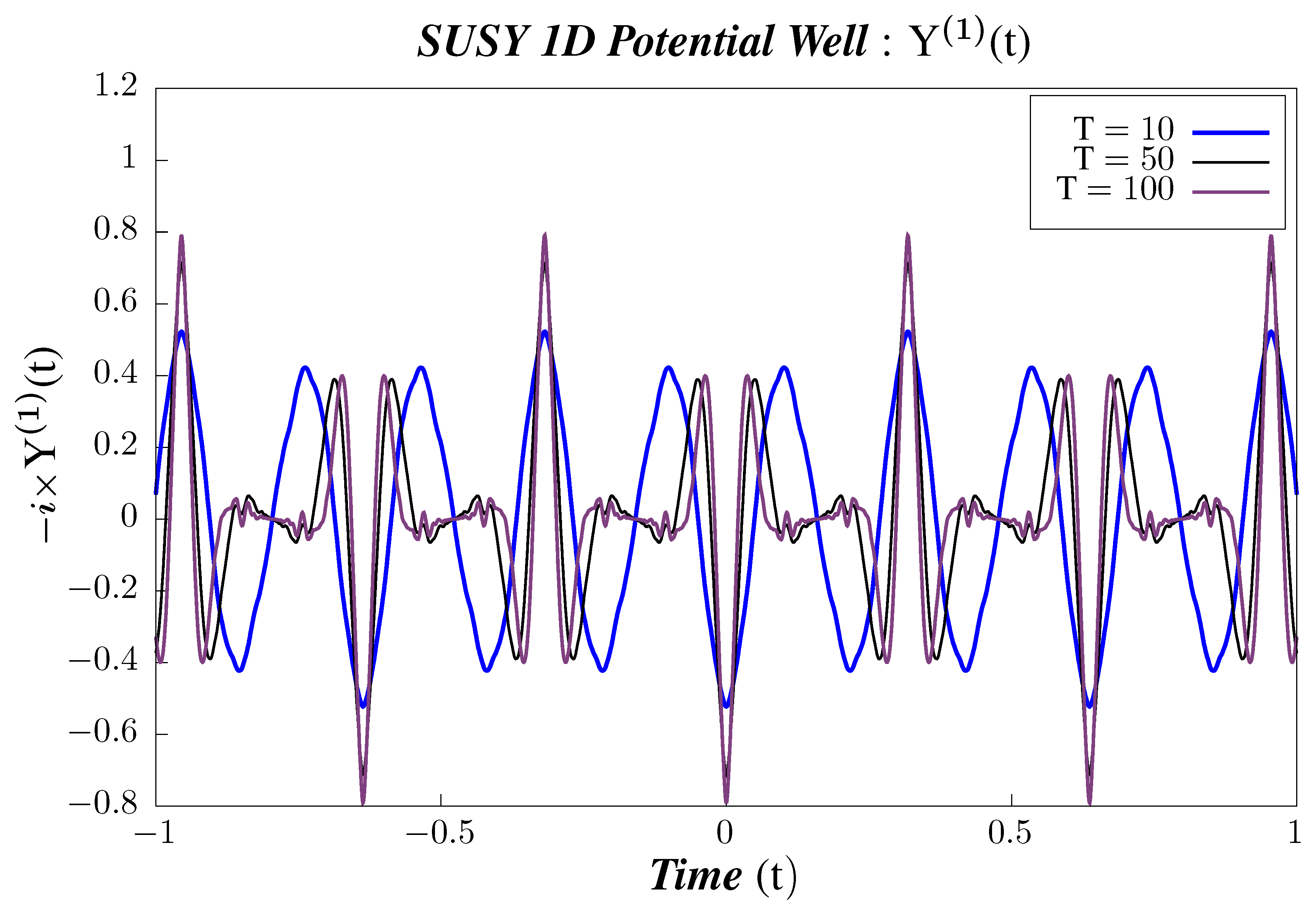
  • Study B:
    The time dependence of 2-point and 4-point canonical correlators for three different temperatures: T = 10 , T = 50 , T = 100 at fixed time t = 0.5 . We have chosen units such that the Boltzmann Constant, k B = 1 , so that the inverse temperature, β = 1 / T . This demonstrates the comparative behavior of canonical correlators for different temperature under time evolution.
  • Study C:
    The temperature dependence of the 2-point and 4-point canonical correlators in the temperature range: 10 T 100 . This demonstrates the explicit temperature dependence of the canonical correlators.
Technically, one has to take the full infinite-dimensional Hilbert Space associated with the Supersymmetric 1D Potential Well for computing the correlators, but it is not possible to do that in a numerical evaluation; hence, one must choose some finite number of states in the Hilbert Space. This choice of a finite value of total number of states will result in an error, and this kind of error is known as Truncation Error. The terminology refers to the fact that the error is arising because we have truncated the number of states to a finite value. Here, we have chosen the truncation to be such that all states N trunc = 10 for numerical evaluation.
From the eigenstate representations for the correlators: y m ( 1 , 2 , 3 ) ( t 1 , t 2 ) , Y ( 1 , 2 , 3 ) ( t 1 , t 2 ) , c m ( 1 , 2 , 3 ) ( t 1 , t 2 ) , and C ( 1 , 2 , 3 ) ( t 1 , t 2 ) given in Section 5.8, we know that they depend only on t 1 t 2 ; hence, we have defined t = t 1 t 2 . So, the negative values of t refer to the case of t 2 > t 1 , and so on. We proceed to the discussion of obtained numerical results.
To make any bold comments about whether we are observing randomness or not, we need to take the commutator brackets as operators O i and then calculate
O i = O i 2 β O i β 2
and check whether O i depends on time t or not. If it does not, then what we have is just statistical fluctuation, which is arising from the inherent quantum nature of the systems and not from randomness. For example: Consider a QHO which has x 0 , but it is also independent of time; this means that, at each instant of time, if we take a large number of copies, then there will be some statistical variation in the values of x across different copies, but that variation will be found exactly the same at each instant of time. If O i = f ( t ) , then it is indeed a true signature of quantum randomness, perhaps depending on functional form of f ( t ) . Since we have calculated both O i 2 β and O i β , it is really easy to check for any signature of randomness. Furthermore, we can use the same method to calculate higher moments than O i and get more and more sensitive measurements for randomness, which is helpful if the f ( t ) above turns out to be some simple periodic function, like f ( t ) cos a t , and we are not satisfied with it because we have really sensitive and amazing technology which can probe for even finer randomness signatures.
To elaborate further, consider the following. We do not really know what quantum uncertainty is; hence, to work with it, we replace it by statistical uncertainty using ensembles, and so on. Then, uncertainty of an operator O i represents its fluctuation across ensembles, and it is not really a true measure of randomness. The fluctuation is merely a sampling fluctuation. Say we take an ensemble consisting of 10,000 copies of a system, then the uncertainty tells us the variation in the measured value of O i across the copies / ensemble at a particular time. Now, if we obtain the O i as a function of time, then we can easily probe for randomness depending on the sensitivity of our instrument. If our instrument is really sensitive, then we can even use higher moments to check for stronger and stronger conditions of randomness. Obtaining O i as a function of time means that the fluctuation itself is changing; hence, this can be a true signature of randomness, which, of course, depends on what kind of function we get.

11.1. Supersymmetric 1D Infinite Potential Well

For numerical evaluation, we have chosen: L = 1 & 2 m = 1 , where L is the length of the box in which a particle of mass m is confined. We also consider = 1 .
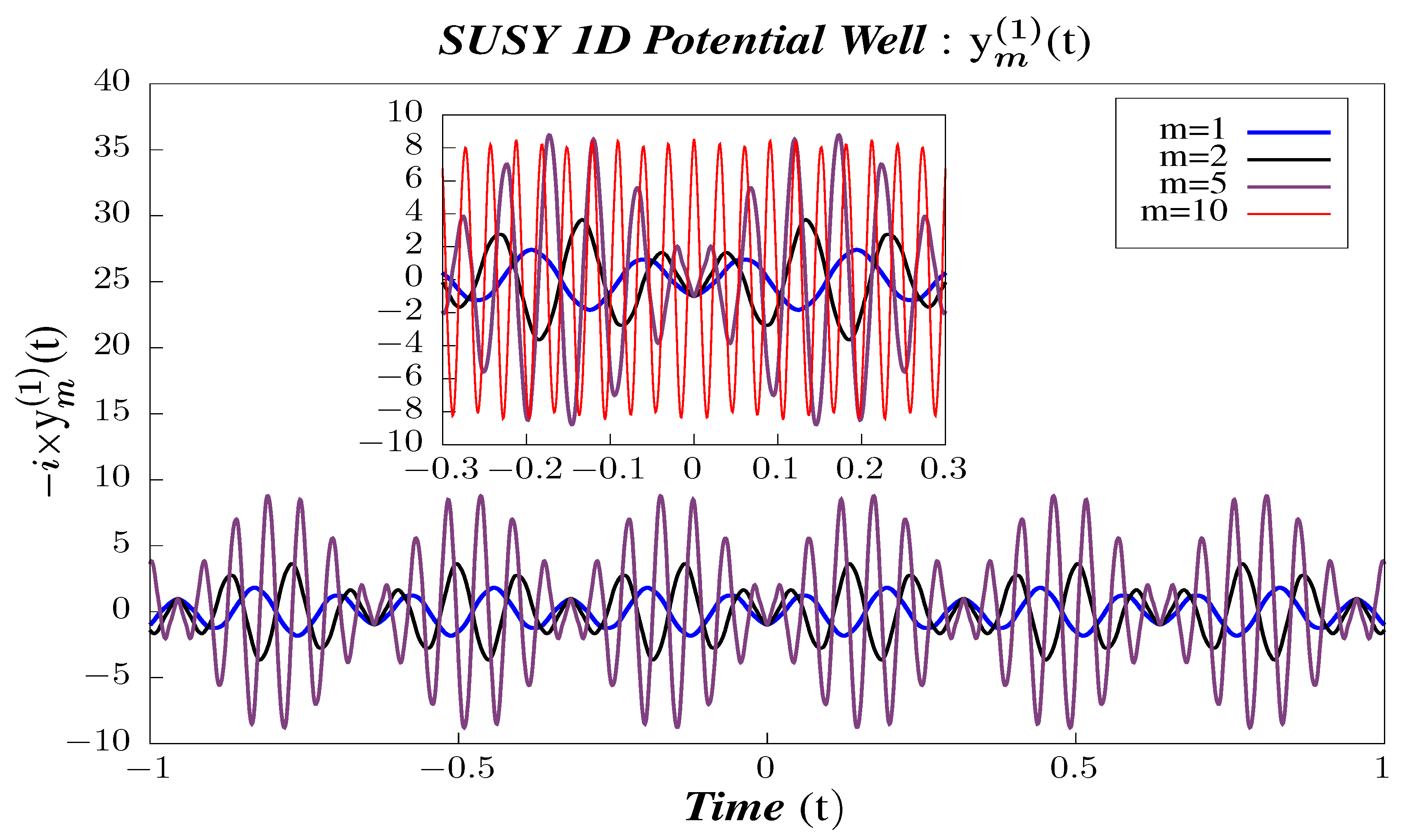
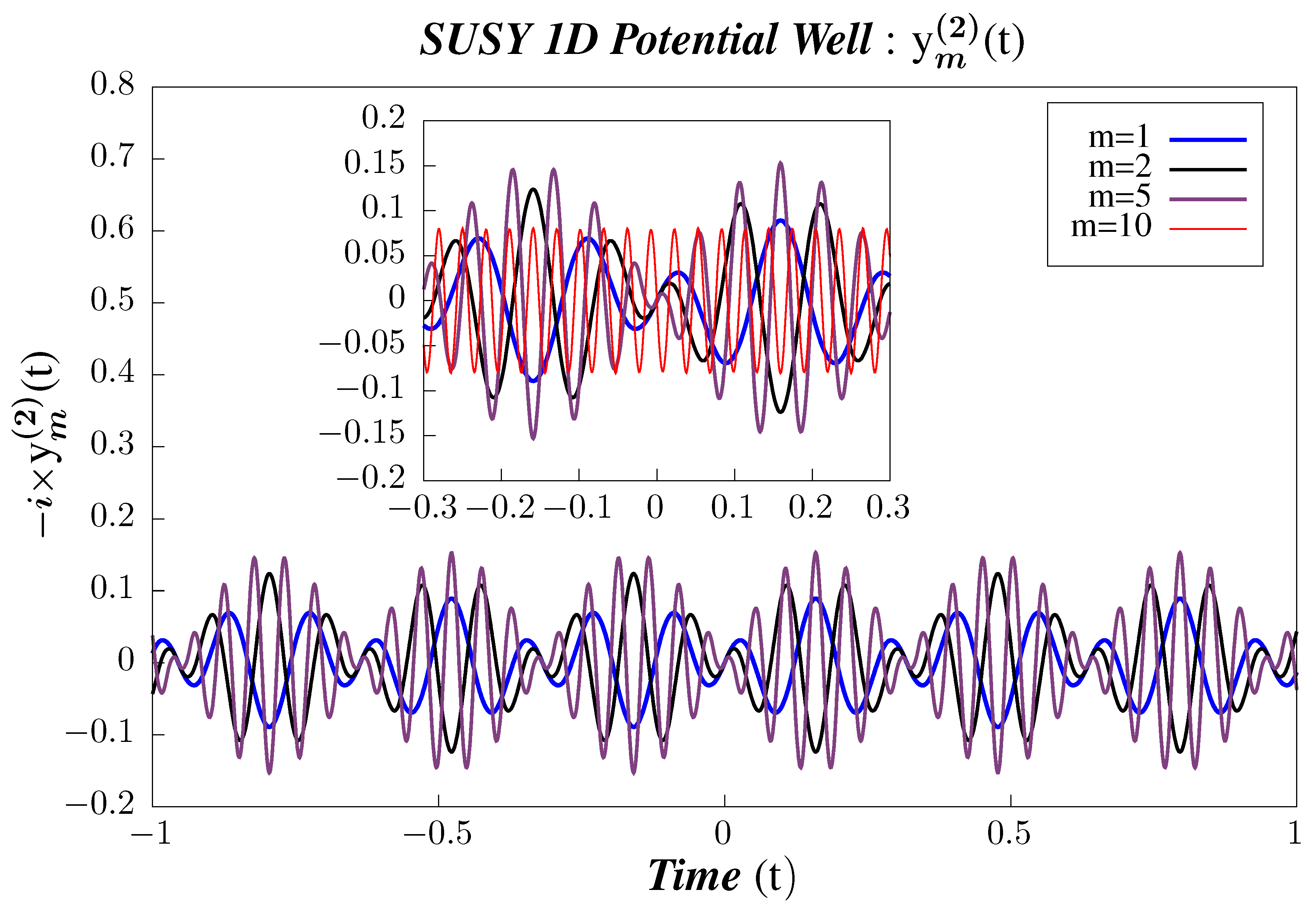
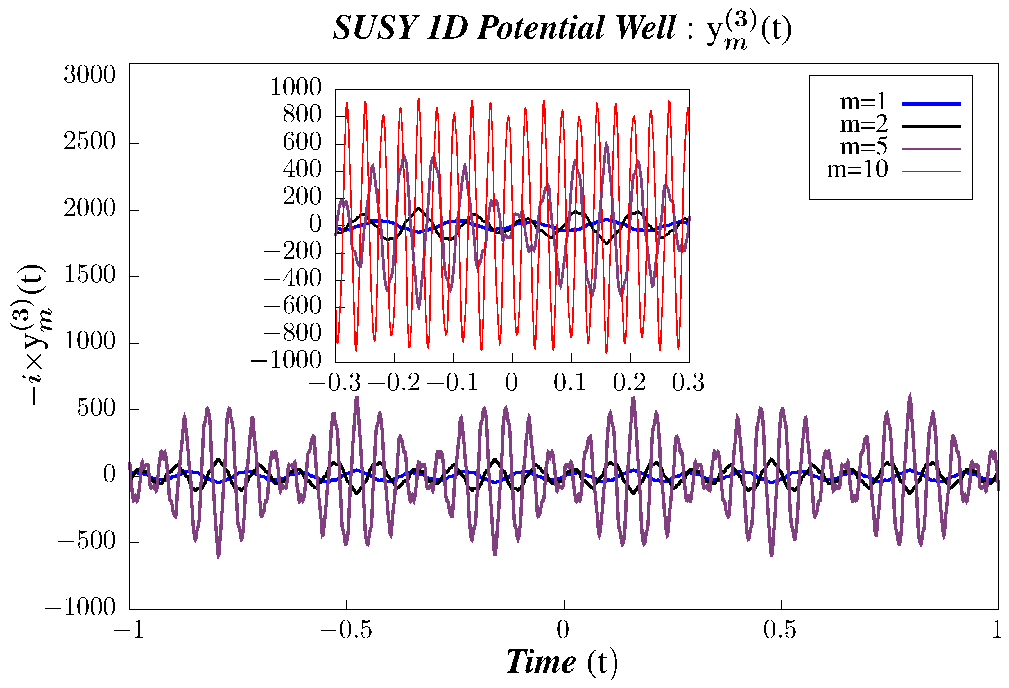
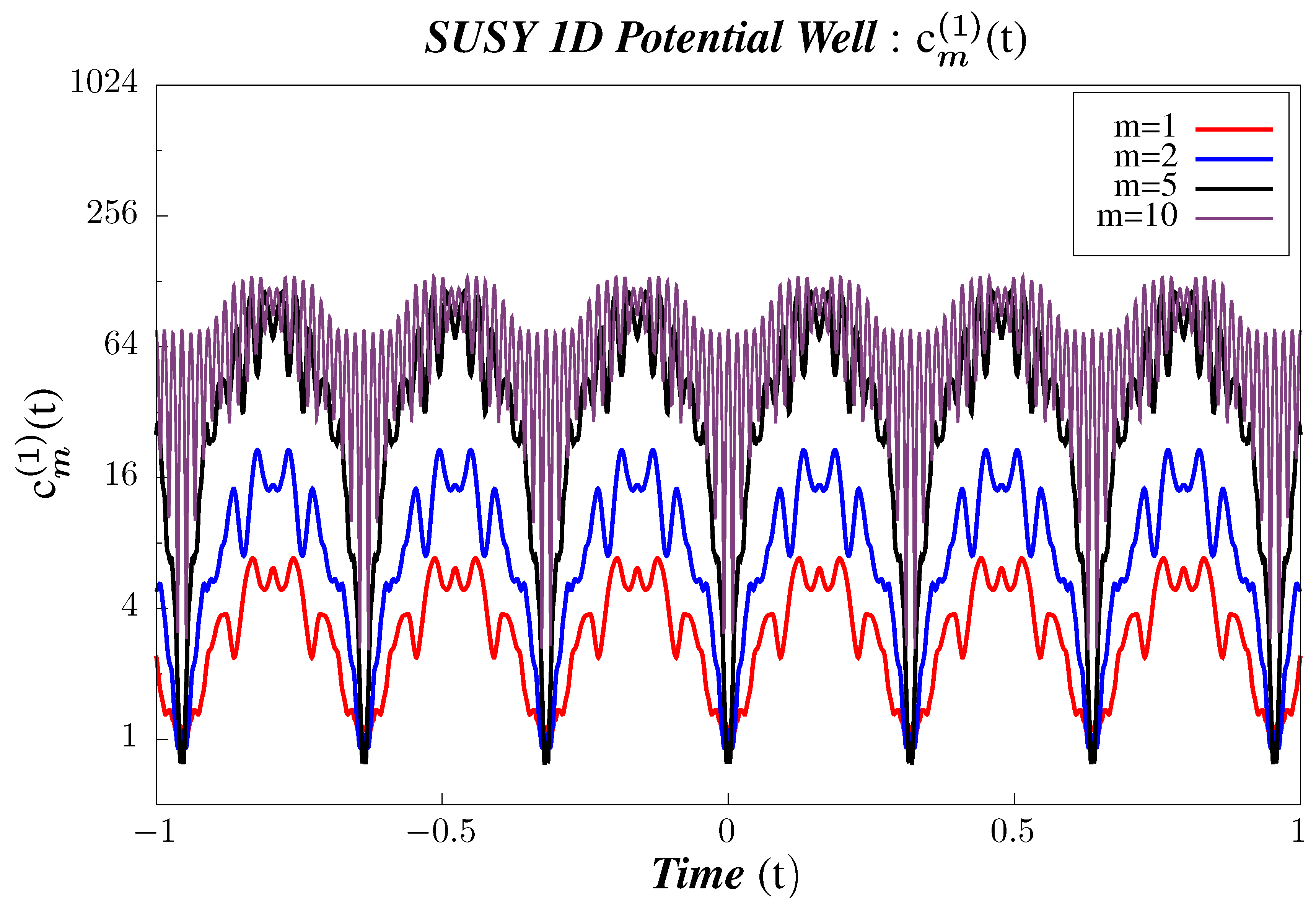
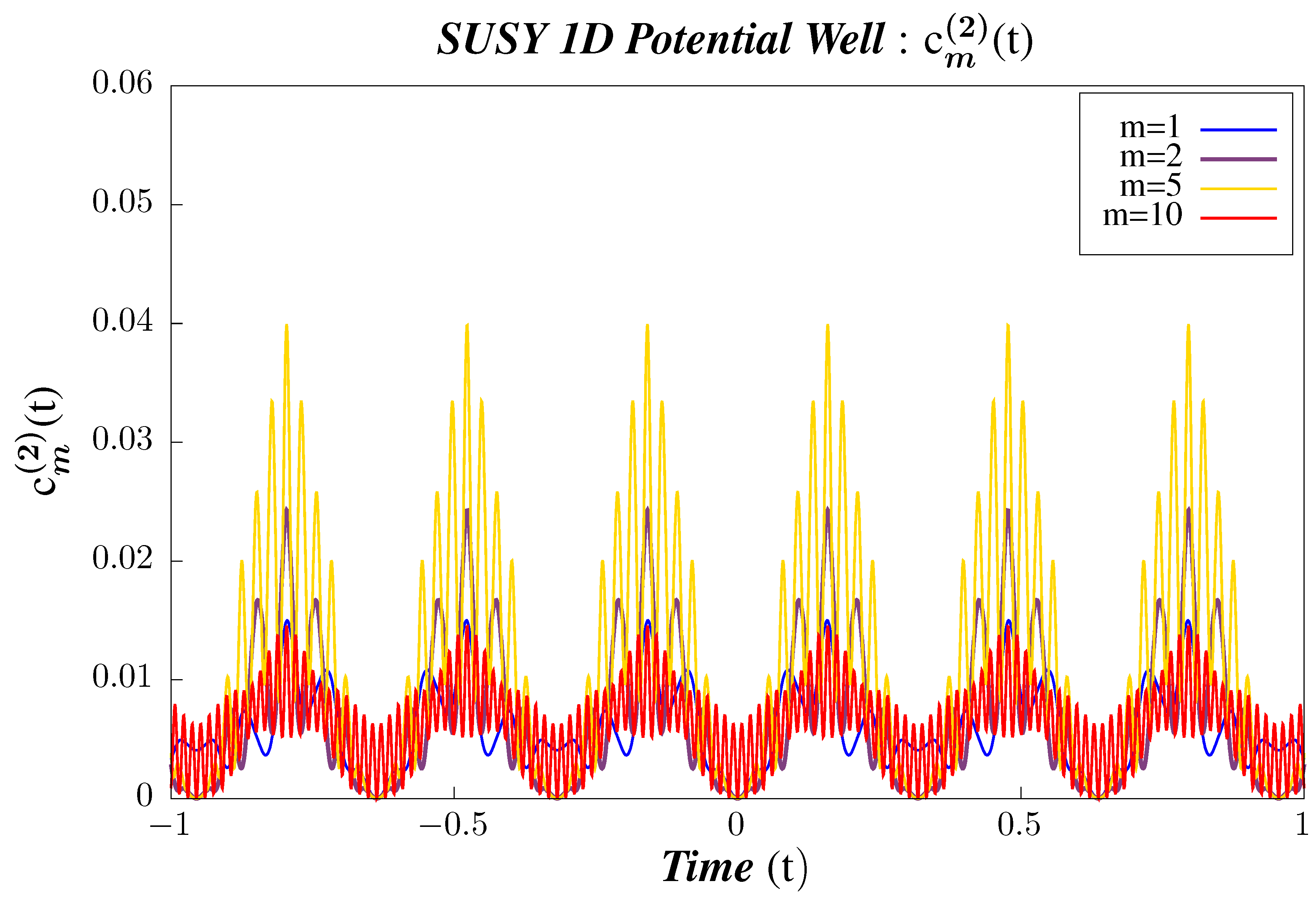
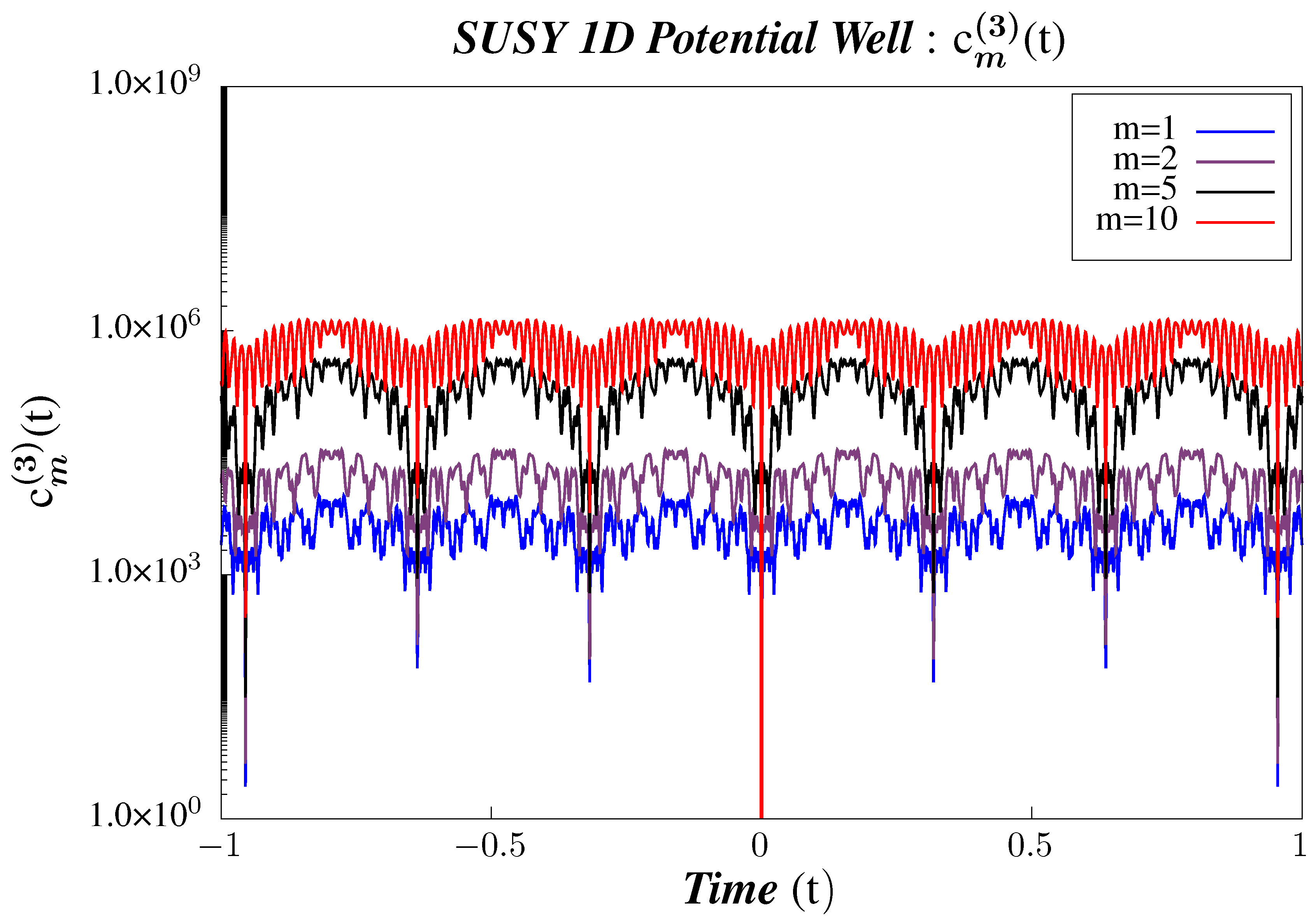
  • In Figure 5, Figure 6 and Figure 7, we perform Study A on the 2-point micro-canonical correlators y m ( 1 , 2 , 3 ) ( t 1 , t 2 ) for Supersymmetric 1D Infinite Potential Well.
    -
    We observe that the correlators y m ( 1 , 2 , 3 ) ( t 1 , t 2 ) are periodic and that their periodicity does not vary with the state. For the correlator y m ( 1 ) ( t 1 , t 2 ) , the periodicity is t 0.65 . At present, there are no studies for the non-Supersymmetric case for y m ( 2 , 3 ) ( t 1 , t 2 ) , and we plan to do the same in a work which is to appear very shortly.
    -
    The amplitude of the correlators increases with increasing m, which primarily comes about because we have:
    i × y m ( 1 ) ( t 1 , t 2 ) E m k = E m E k = π 2 m 2 k 2
    in the correlator’s eigenstate representation, which increases with increasing state number.
    -
    It is also observed that, with a higher and higher excited state, the number of nodes increases and takes on the shape of a wave-packet. This is so because, as we go to higher and higher excited states, the high frequency modes become more and more prominent. So, the comparison of the scaling of the number of nodes here with non-Supersymmetric case is also important job to perform in near future.
    -
    In the insets of Figure 5, Figure 6 and Figure 7, we have also plotted y 10 ( 1 , 2 , 3 ) ( t 1 , t 2 ) to draw a contrast of the boundary / truncation state with the other states. The m = 10 correlators are lacking in features, sometimes deceptively so, as compared to the other states, which should come as no surprise because we have set our truncation at N trunc = 10 . Furthermore, this state appears to violate the properties shown by other intermediate states, but, in fact, this is merely an artefact of m = 10 being the truncation state and that contribution of states with m > 10 could not be accommodated in the calculations for m = 10 .
    -
    The correlators y m ( 2 , 3 ) ( t 1 , t 2 ) largely follow the same patterns and behavior as shown by y m ( 1 ) ( t 1 , t 2 ) with two exceptions. First, the amplitude for y m ( 2 ) ( t 1 , t 2 ) correlator is suppressed, whereas that of y m ( 3 ) ( t 1 , t 2 ) is amplified, both by a factor of O ( 10 1 ) , as compared to y m ( 1 ) ( t 1 , t 2 ) . This comes from the absence of E m k factor in y m ( 2 ) ( t 1 , t 2 ) and the presence of an additional E m k factor in y m ( 3 ) ( t 1 , t 2 ) as compared to y m ( 1 ) ( t 1 , t 2 ) . Second is the contrasting behavior in the symmetry properties in t, whereas y m ( 1 ) ( t 1 , t 2 ) is symmetric in t, and y m ( 2 , 3 ) ( t 1 , t 2 ) are anti-symmetric.
  • We present the results of performing Study B and Study C on 2-point canonical correlators Y ( i ) ( t 1 , t 2 ) as follows:
    -
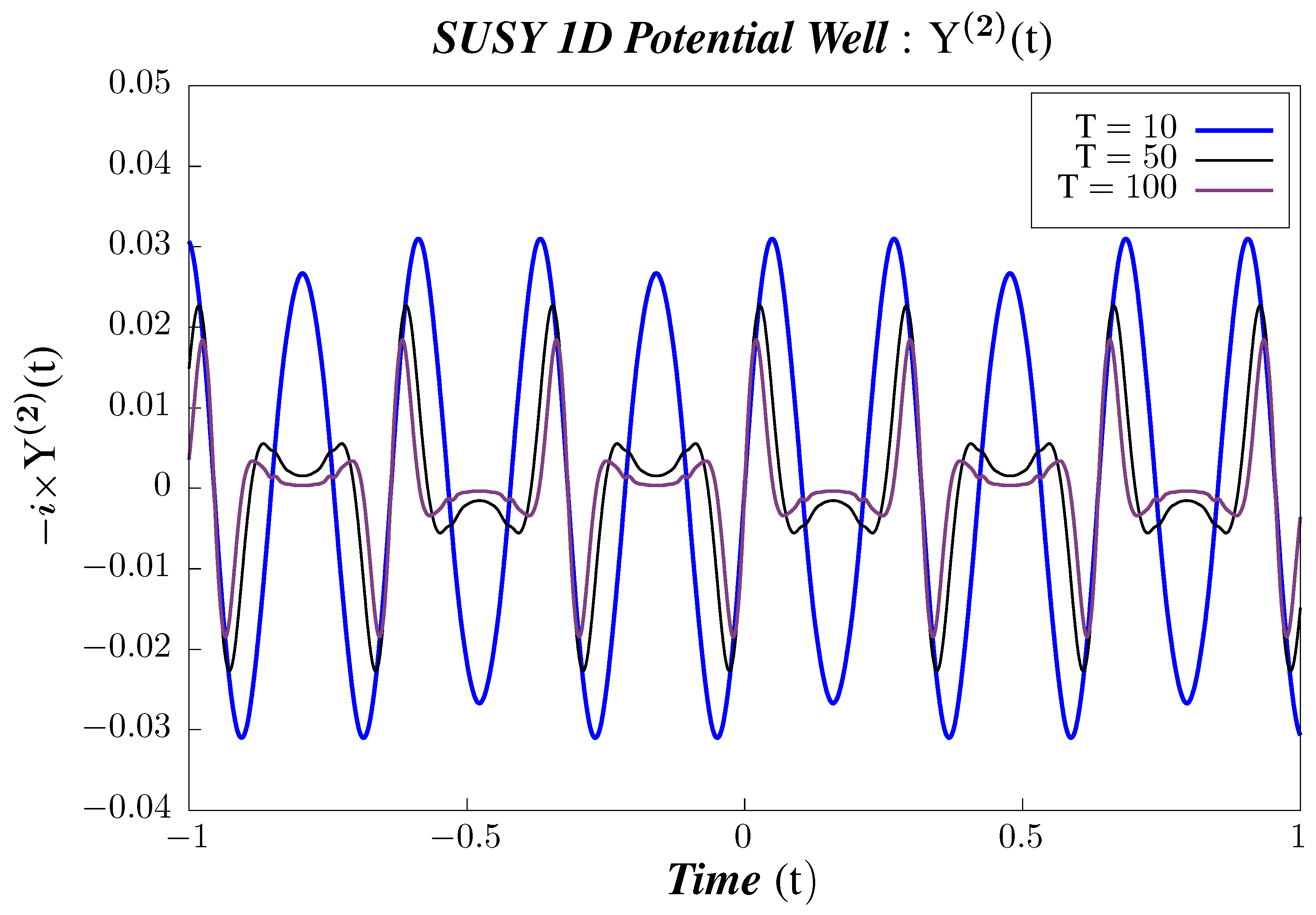
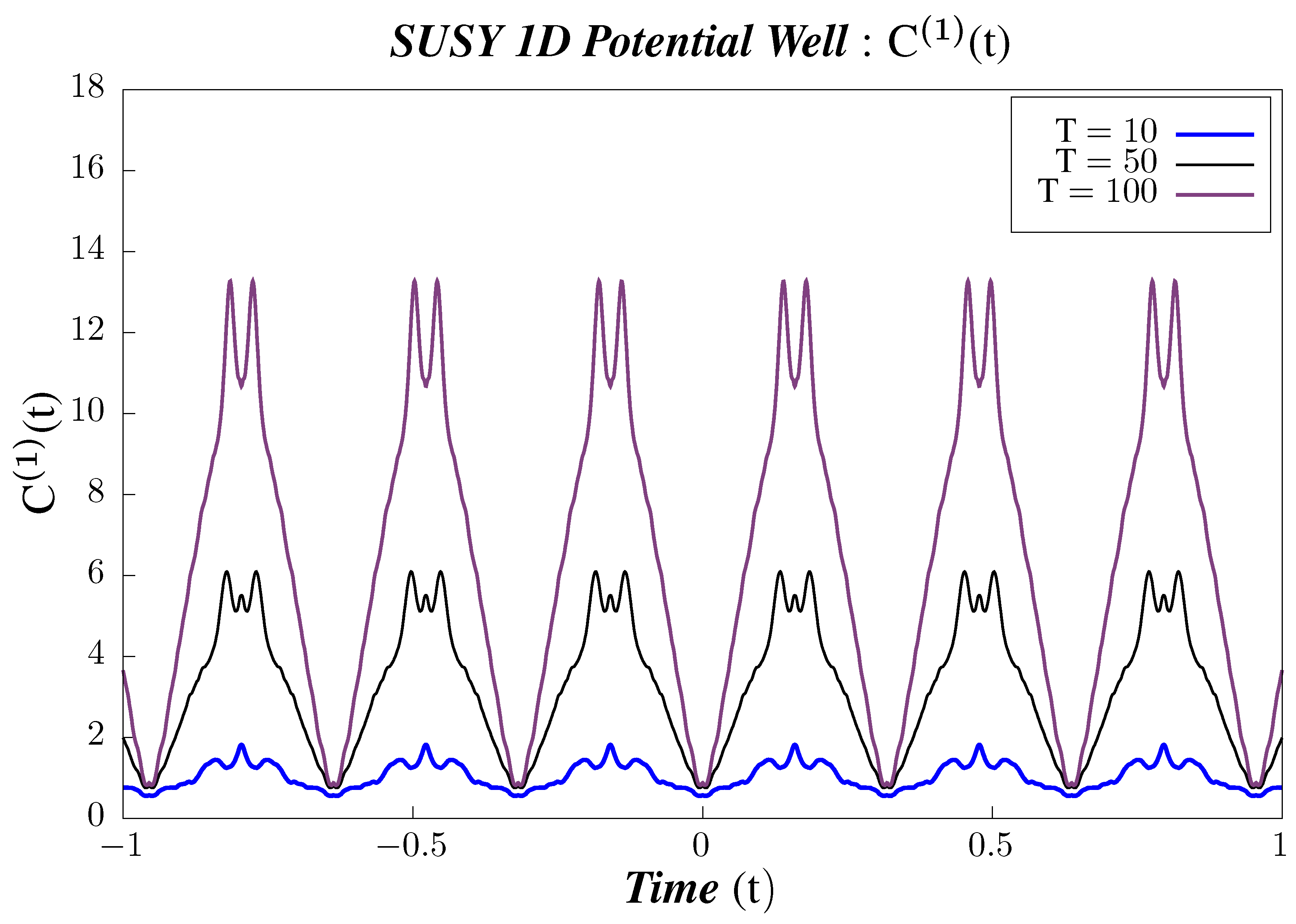
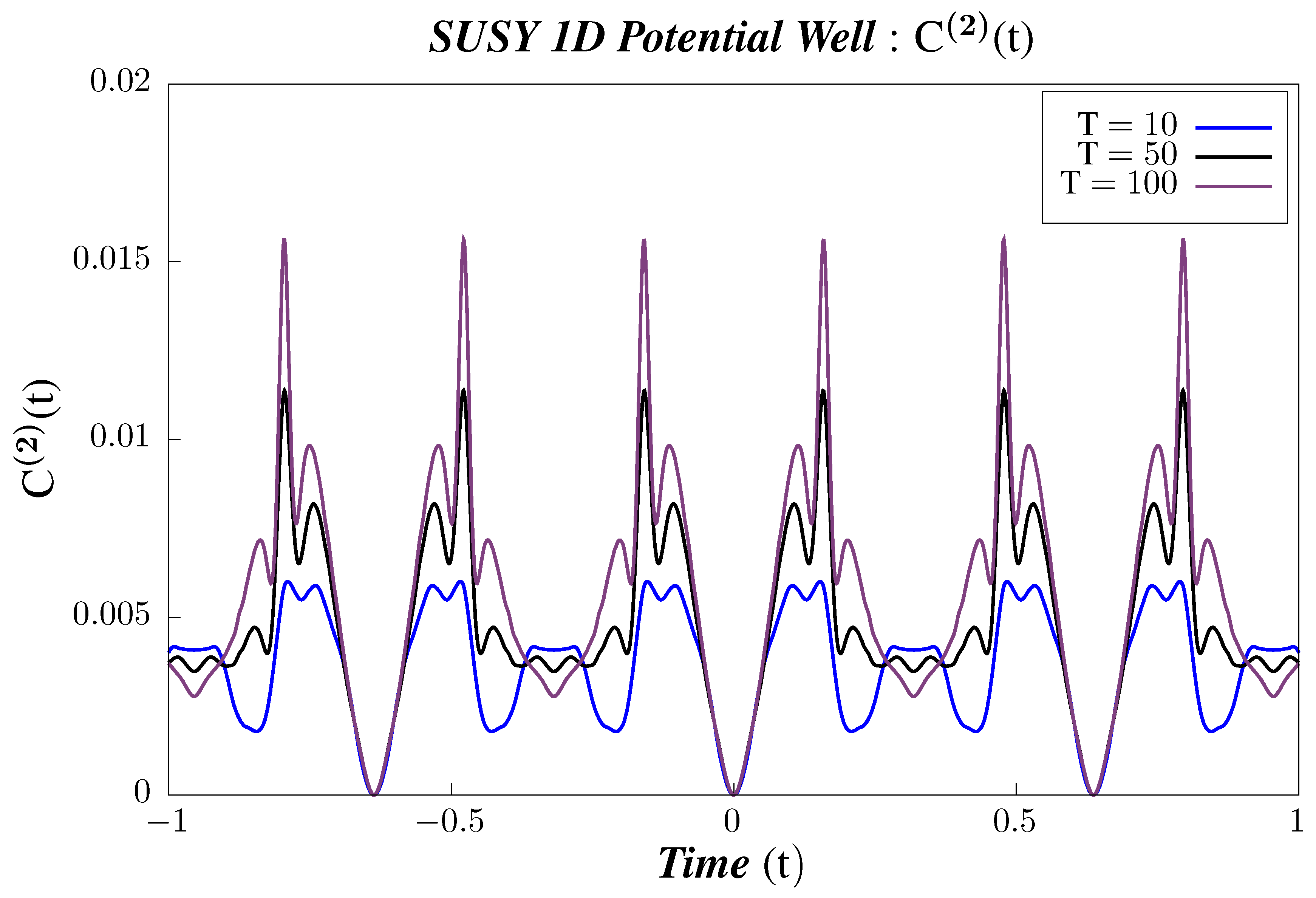
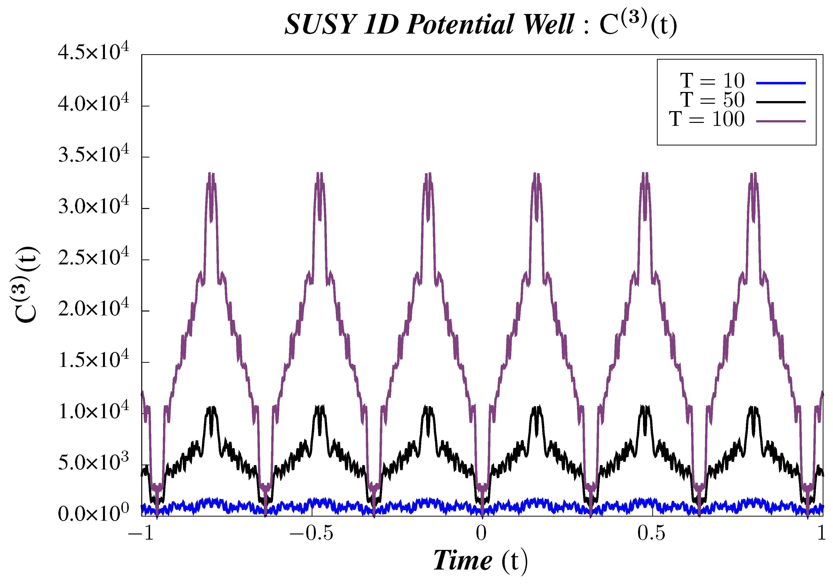
    In Figure 8, Figure 9 and Figure 10, we perform Study B on the 2-point canonical correlators Y ( 1 , 2 , 3 ) ( t 1 , t 2 ) . We observe that the correlators shows periodic behavior for the different chosen values of temperature. We observe that, for Y 1 ( t 1 , t 2 ) , the mid temperature value 50 shows the minimum amplitude, whereas lower value of temperature (10) has greater amplitude. However, there is a sudden increase in the amplitude of the correlator for temperatures in the higher value range as can be seen from Figure 8. In correlators Y 2 ( t 1 , t 2 ) and Y 3 ( t 1 , t 2 ) , however, we follow a gradual pattern of decreasing amplitude with increasing in temperature, as observed from Figure 9 and Figure 10. To have a better understanding of the temperature dependence of the 2-point correlators, we plot them with varying temperatures, keeping the time constant.
    -
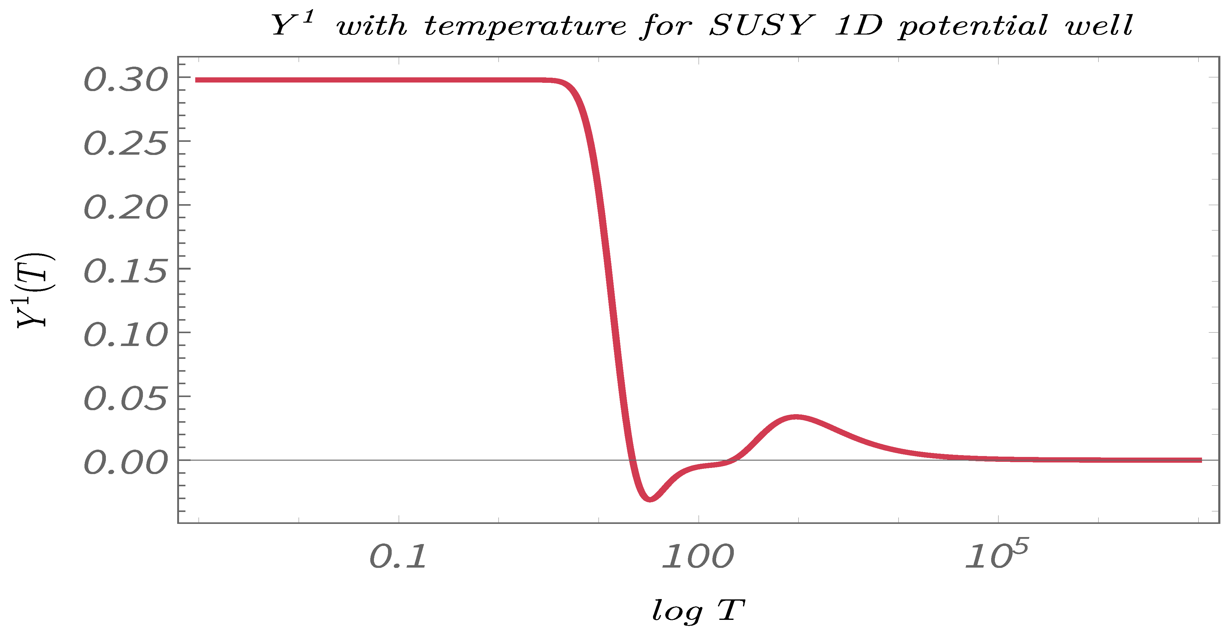
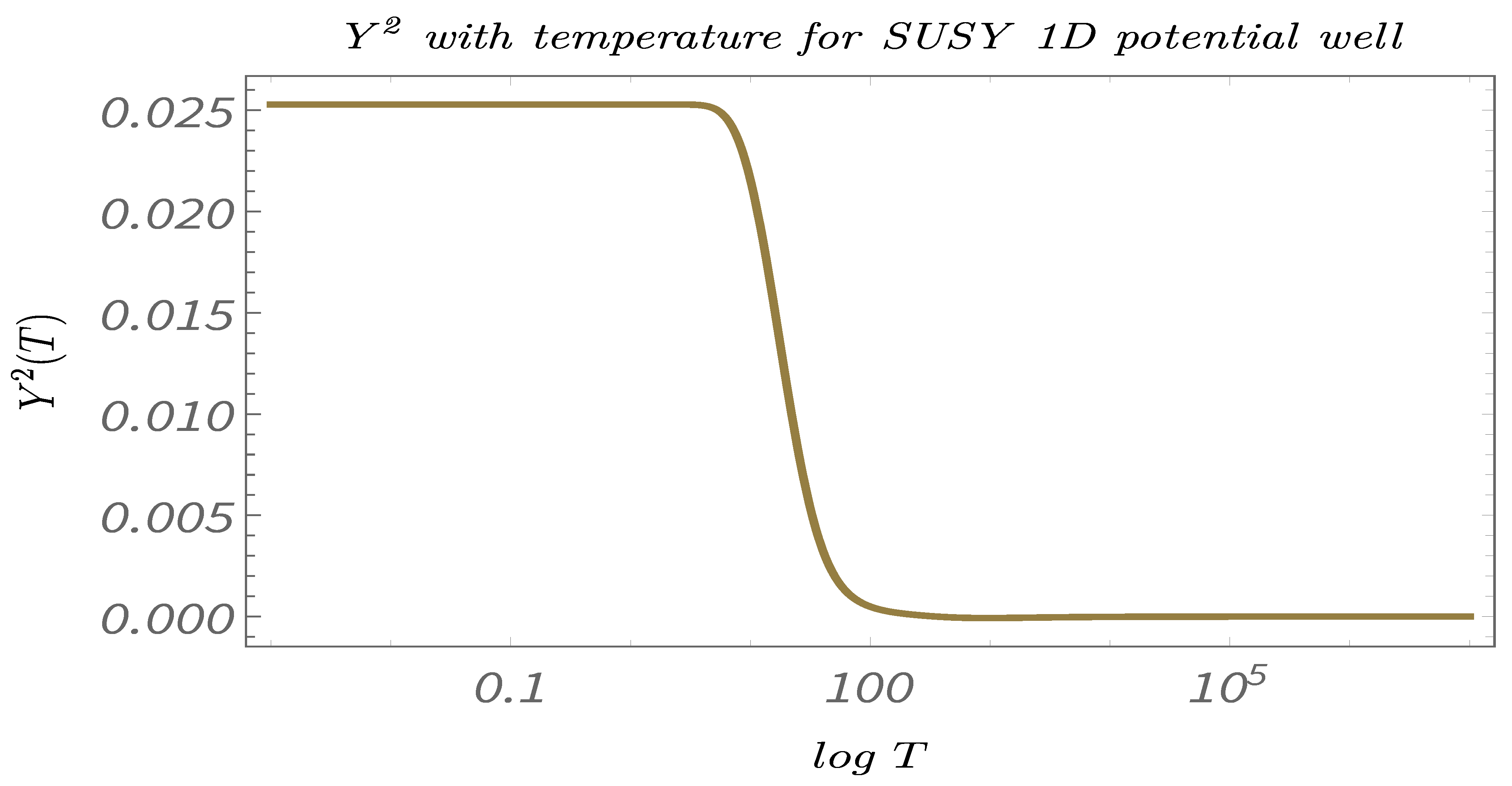
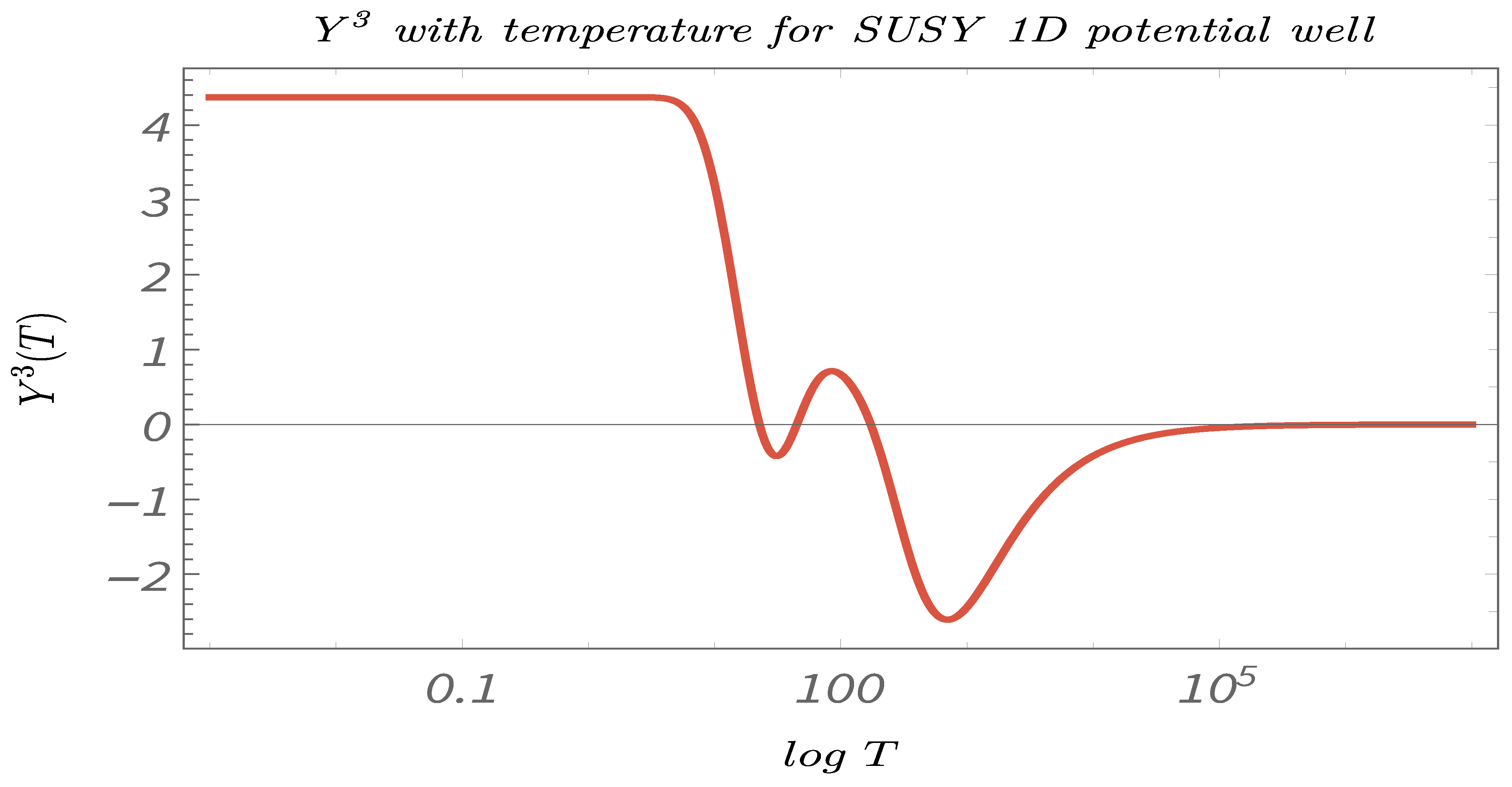
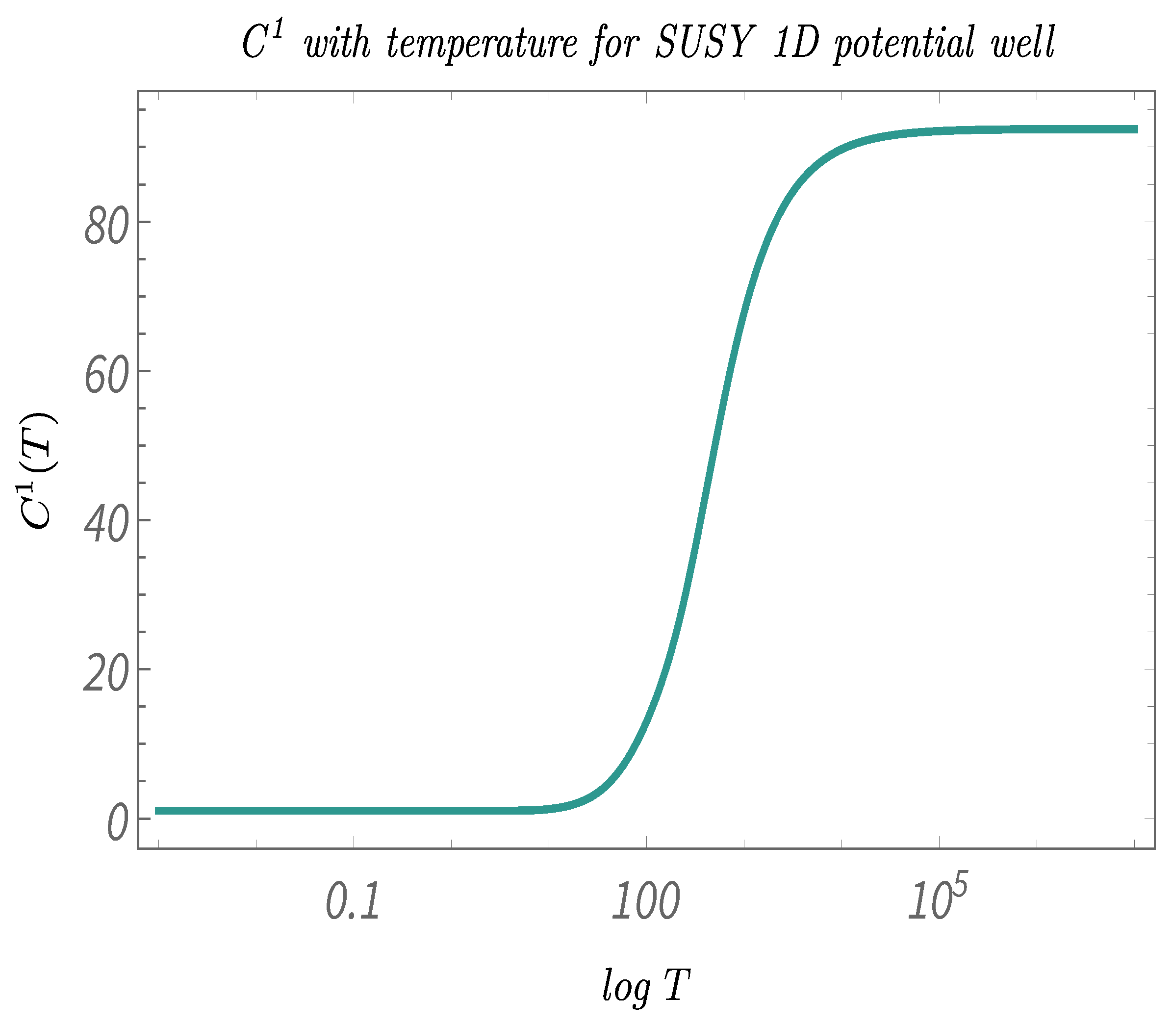
    In Figure 11, Figure 12 and Figure 13, we perform Study C on the 2-point canonical correlators Y ( 1 , 2 , 3 ) ( t 1 , t 2 ) . We plot, respectively, Y ( 1 , 2 , 3 ) ( t 1 , t 2 ) , which are the thermal or canonical correlators corresponding to y m ( 1 , 2 , 3 ) ( t 1 , t 2 ) , respectively, with respect to temperature. It is clearly visible that, for very low temperatures, the canonical correlators are constant. However, after a certain value of the temperature, the correlators decays rapidly and falls off to zero within a small temperature range.
    -
    In Figure 14, Figure 15 and Figure 16, we perform Study A on the 4-point micro-canonical correlators c m ( 1 , 2 , 3 ) ( t 1 , t 2 ) for Supersymmetric 1D Infinite Potential Well.
    -
    We observe that the correlators c m ( 1 , 2 , 3 ) ( t 1 , t 2 ) are periodic and that their periodicity does not vary with the state. For the correlator c m ( 1 ) ( t 1 , t 2 ) , the periodicity is t 0.35 , which is roughly half of the corresponding 2-point micro-canonical correlator. We note that this is approximately the same periodicity, within numerical error, observed in the case of non-Supersymmetric 1D Infinite Potential Well as obtained by Hashimoto et al. [90]. Hence, we conclude that introducing Supersymmetry in integrable QMcal models does not affect the periodicity of 4-point micro-canonical correlators. At present, there are no studies for the non-Supersymmetric case for c m ( 2 , 3 ) ( t 1 , t 2 ) , and we plan to do the same in a work which is to appear very shortly.
    -
    Other properties of c m ( i ) ( t 1 , t 2 ) are much like y m ( i ) ( t 1 , t 2 ) . We observe a similar increase in the amplitude of the correlators with increasing m. The scaling of amplitudes in the case of 4-point micro-canonical correlators is with a factor of O ( 10 4 ) instead of a factor O ( 10 1 ) as is the case with y m ( i ) ( t 1 , t 2 ) such that the relative order of amplitudes can be arranged as: c m ( 3 ) ( t 1 , t 2 ) > c m ( 2 ) ( t 1 , t 2 ) > c m ( 1 ) ( t 1 , t 2 ) .
    -
    All c m ( i ) ( t 1 , t 2 ) are symmetric about t = 0 , which means that, to these 4-point micro-canonical correlators, it does not matter whether t 1 > t 2 or t 1 < t 2 .
    -
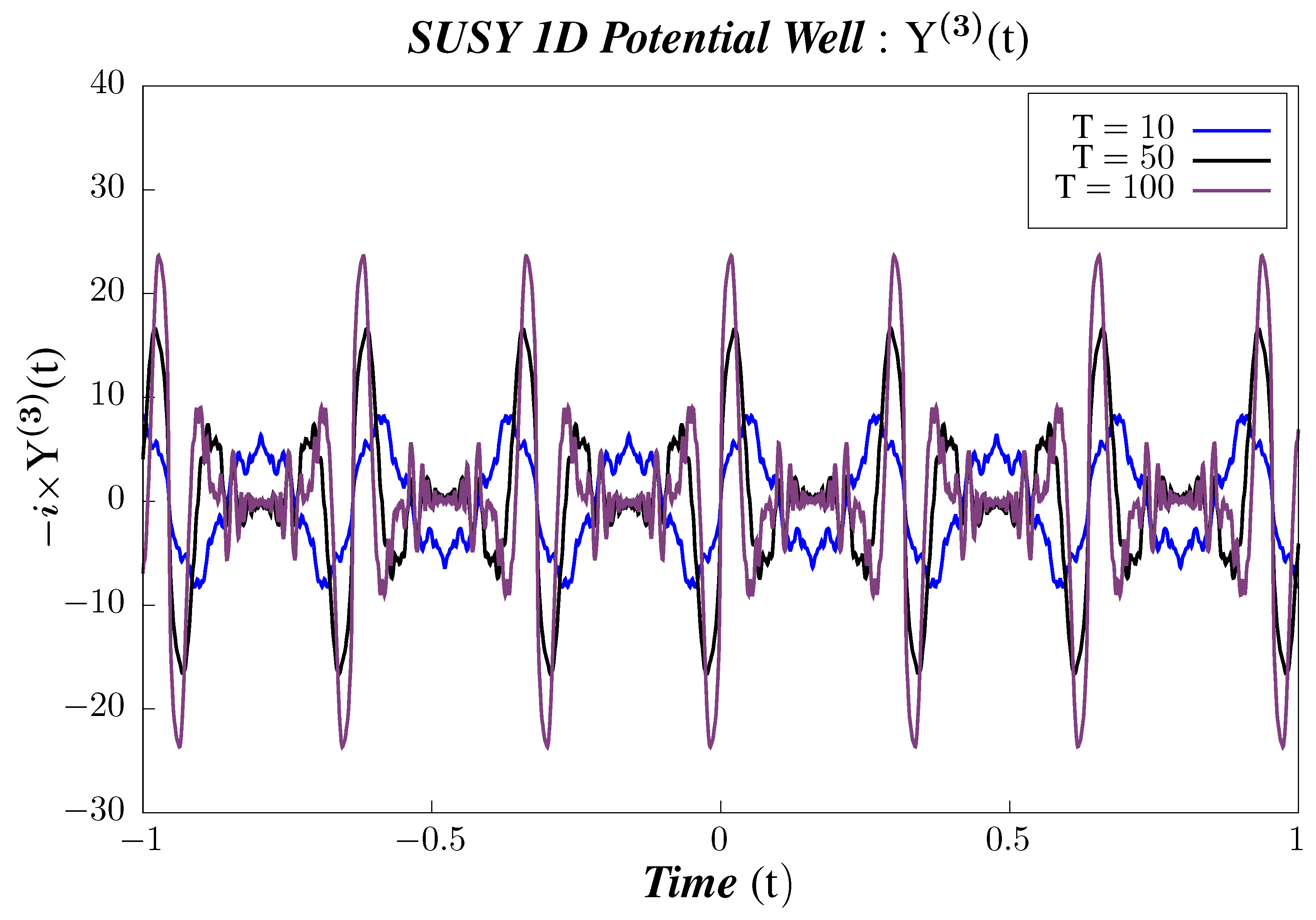
    In Figure 17, Figure 18 and Figure 19, we perform Study B on the 4-point canonical correlators. We plot the 4-point canonical correlators for three different temperatures. We observe that all the 4-point correlators shows periodic behavior irrespective of the value of the temperature. It is also observed that, for each correlator, the amplitude increases with the increasing temperature. To have a better understanding of the temperature dependence of the 4-point correlators, we plot them with varying temperature, keeping the time constant.
    -
    In Figure 20, Figure 21 and Figure 22, we perform Study C on the 4-point canonical correlators. we plot, respectively, C ( 1 , 2 , 3 ) ( t 1 , t 2 ) , which are the thermal or canonical correlators corresponding to c m ( 1 , 2 , 3 ) ( t 1 , t 2 ) , respectively, with respect to temperature. It is observed that, for low temperatures, the 4-point correlators show negligible value. However, after a certain threshold temperature, the 4-point correlators increases and then saturates to a certain finite value.
  • The temperature-dependent plots for the 2-point and the 4-point canonical correlators suggests that both the 2- and the 4-point canonical correlators are essential if one wants to have a complete understanding of the phenomenon of Quantum randomness. The plots suggests that 2-point correlators are a better probe for understanding Quantum randomness at low temperatures, whereas, at high temperatures, it is actually the 4-point correlators, which is more significant. However, in the mid-temperature range, the 2-point and the 4-point correlators have exactly opposite behavior. Hence, to understand the significance of temperature in this range on any Supersymmetric Quantum mechanical model, having knowledge of both 2- and 4-point correlators is of utmost importance.

11.2. Supersymmetric 1D Harmonic Oscillator

For numerical evaluation, we have chosen: ω = 1 & 2 M = 1 , where ω is the frequency of the oscillator, in which a particle of mass M is confined. We also consider = 1 .
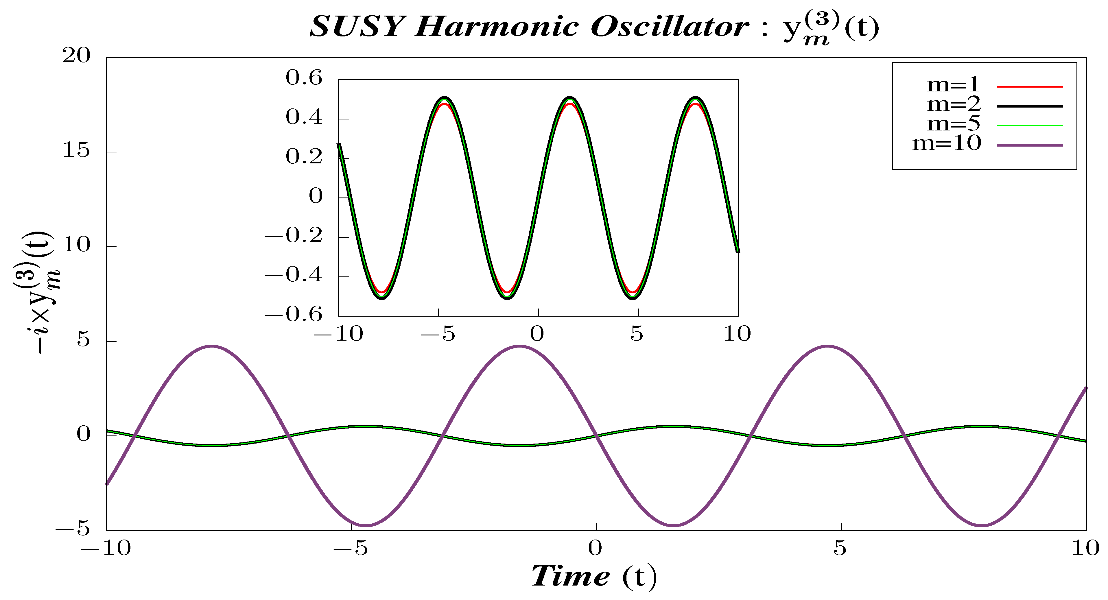
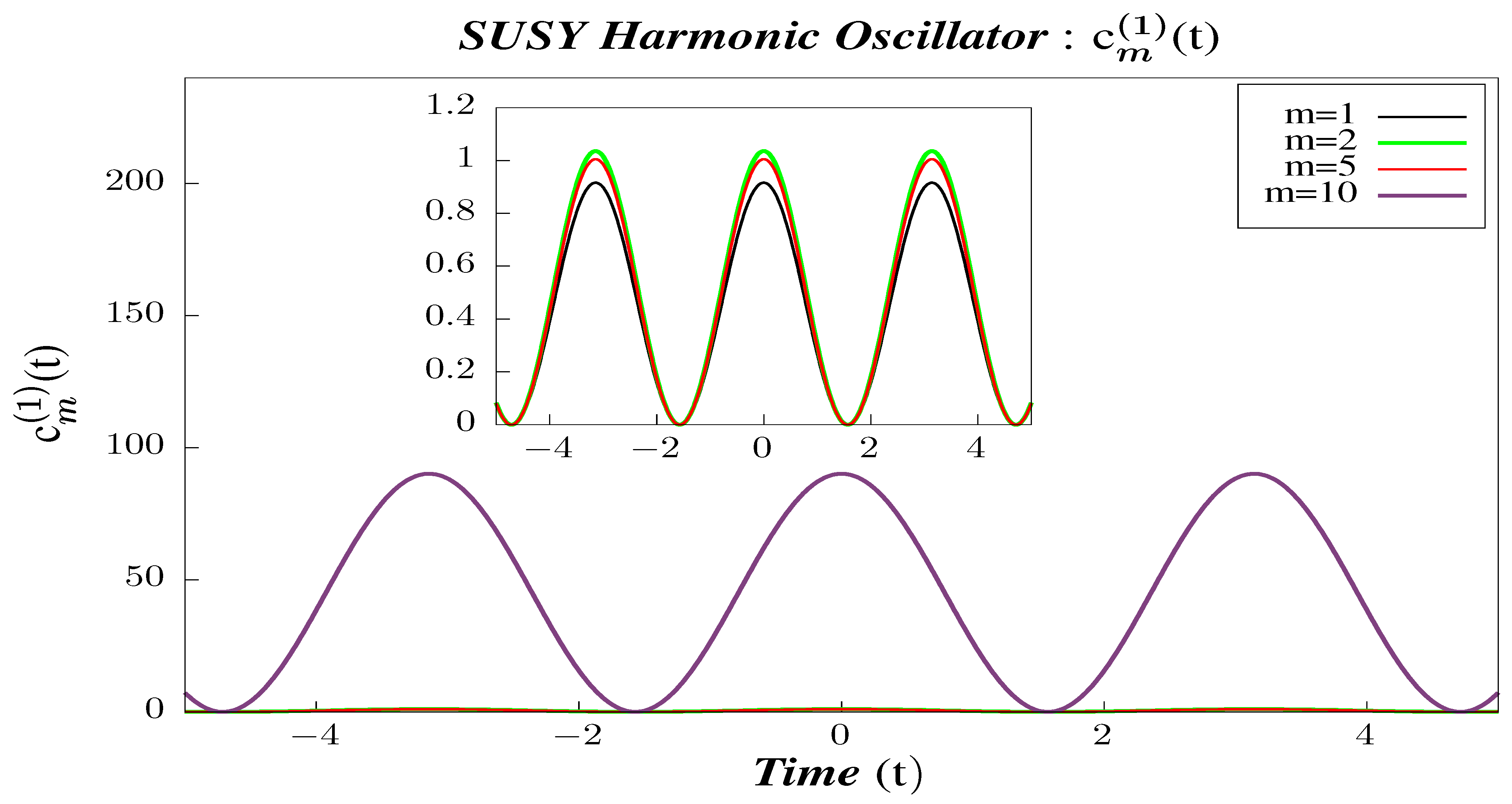
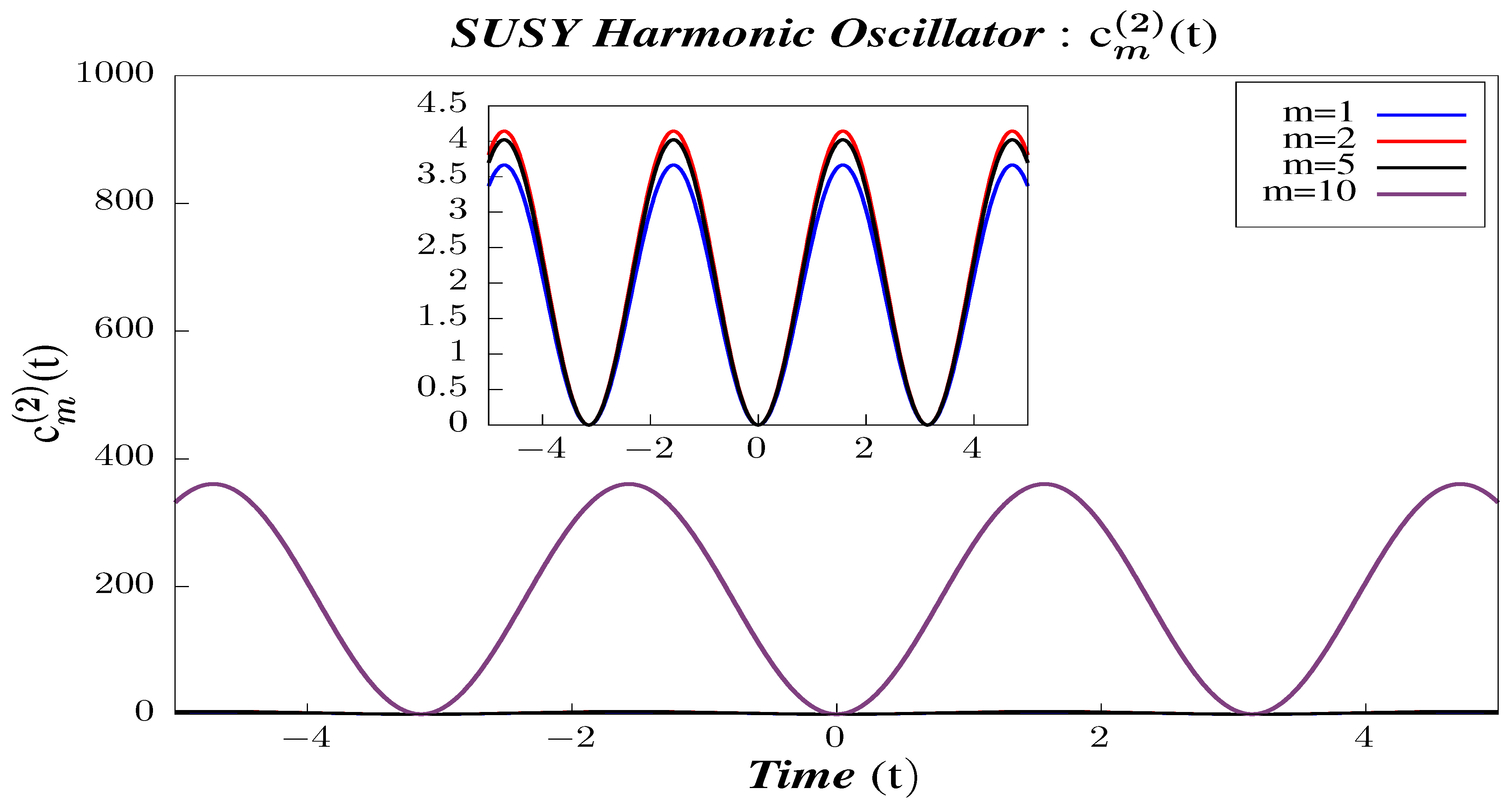
  • In Figure 23, Figure 24 and Figure 25, we perform Study A on the 2-point micro-canonical correlators y m ( 1 , 2 , 3 ) ( t 1 , t 2 ) for Supersymmetric 1D Harmonic Oscillator.
    -
    We observe that the correlators y m ( 1 , 2 , 3 ) ( t 1 , t 2 ) are periodic and that their periodicity does not vary with the state.
    -
    The amplitude of the correlator y m ( 1 ) ( t 1 , t 2 ) initially increases with increasing m, which can be seen from the greater amplitude for m = 2 than the amplitude for m = 1. However, with further increase of m, the amplitude of the correlator shows negligible change, and the amplitudes of the higher states almost overlap. This suggests that, for the lower energy states, the micro-canonical correlators depend on the energy state in which they are calculated. However, this state dependency goes away when calculated for the higher energy states. This can also be understood from the analytical expression obtained for the micro-canonical correlators obtained in Section 6 (calculated for Harmonic Oscillator of unit mass, i.e., M = 1 ). The micro-canonical correlators have a non-trivial state dependence in the form of the factor 1 + m ( m + 1 ) m ( m 1 ) , which reduces simply to 1 for higher energy states.
    -
    In Figure 23, Figure 24 and Figure 25, we have also plotted y 10 ( 1 , 2 , 3 ) ( t 1 , t 2 ) to draw a contrast of the boundary / truncation state with the other states. The m = 10 correlators are lacking in feature, sometimes deceptively so, as compared to the other states, which should come as no surprise because we have set our truncation at N trunc = 10 . Furthermore, this state appears to violate the properties shown by other intermediate states, but, in fact, this is merely an artefact of m = 10 being the truncation state and that contribution of states with m > 10 could not be accommodated in the calculations for m = 10 .
    -
    The correlators y m ( 2 , 3 ) ( t 1 , t 2 ) largely follow the same patterns and behavior as shown by y m ( 1 ) ( t 1 , t 2 ) with two exceptions. First, the amplitude for y m ( 2 ) ( t 1 , t 2 ) correlator is amplified, whereas that of y m ( 3 ) ( t 1 , t 2 ) is suppressed, as compared to y m ( 1 ) ( t 1 , t 2 ) . The order of the amplification of the micro-canonical correlator y m ( 2 ) ( t 1 , t 2 ) is exactly twice the amplitude of y m ( 1 ) ( t 1 , t 2 ) , which is merely a reflection of the fact that the mass of the oscillator has been chosen as 1 / 2 . Similarly, the suppression of y m ( 3 ) ( t 1 , t 2 ) is exactly by the same factor. Second is contrasting behavior in the symmetry properties in t, whereas y m ( 1 ) ( t 1 , t 2 ) is symmetric in t, and y m ( 2 , 3 ) ( t 1 , t 2 ) are anti-symmetric.
    -
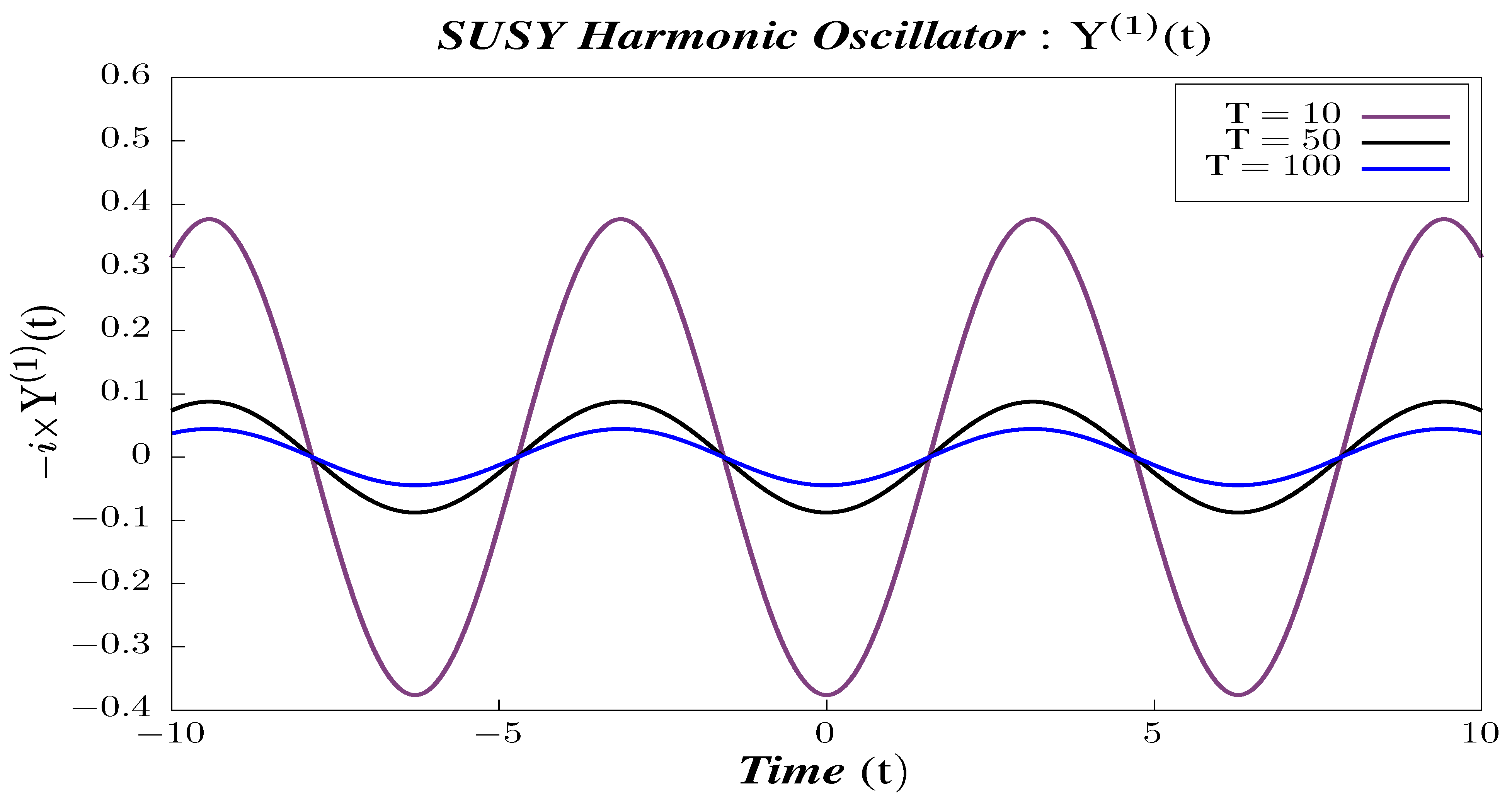
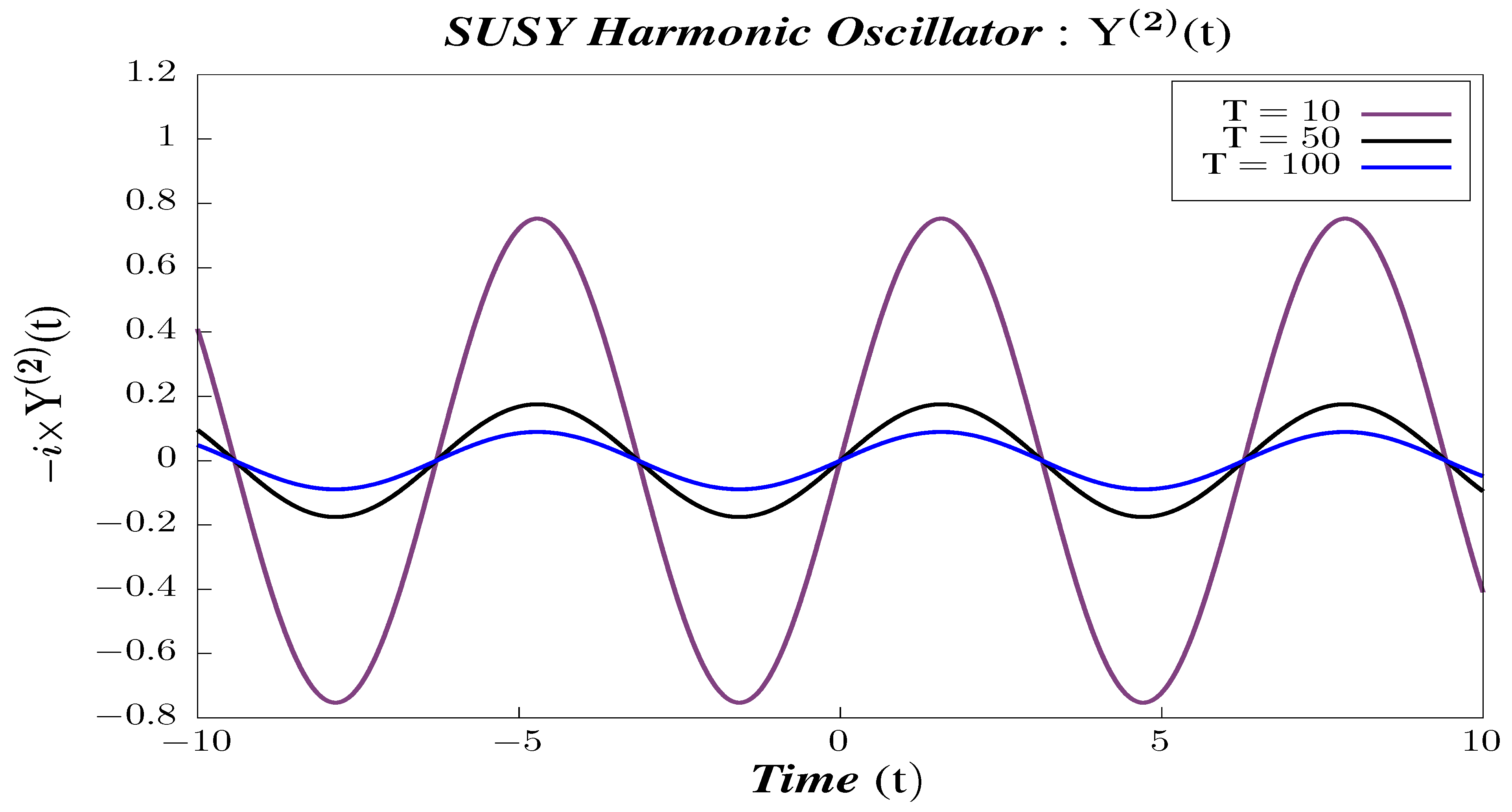
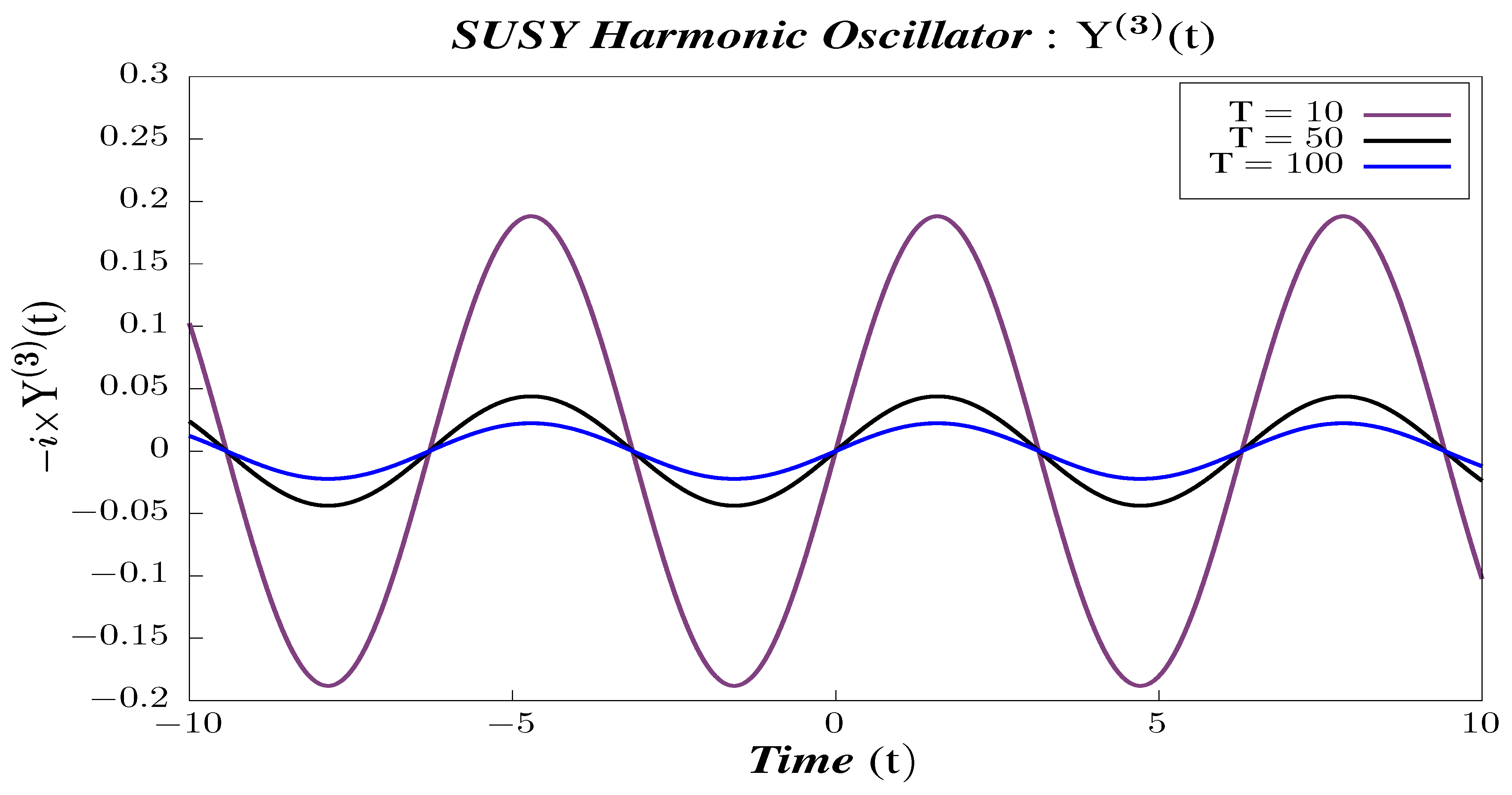
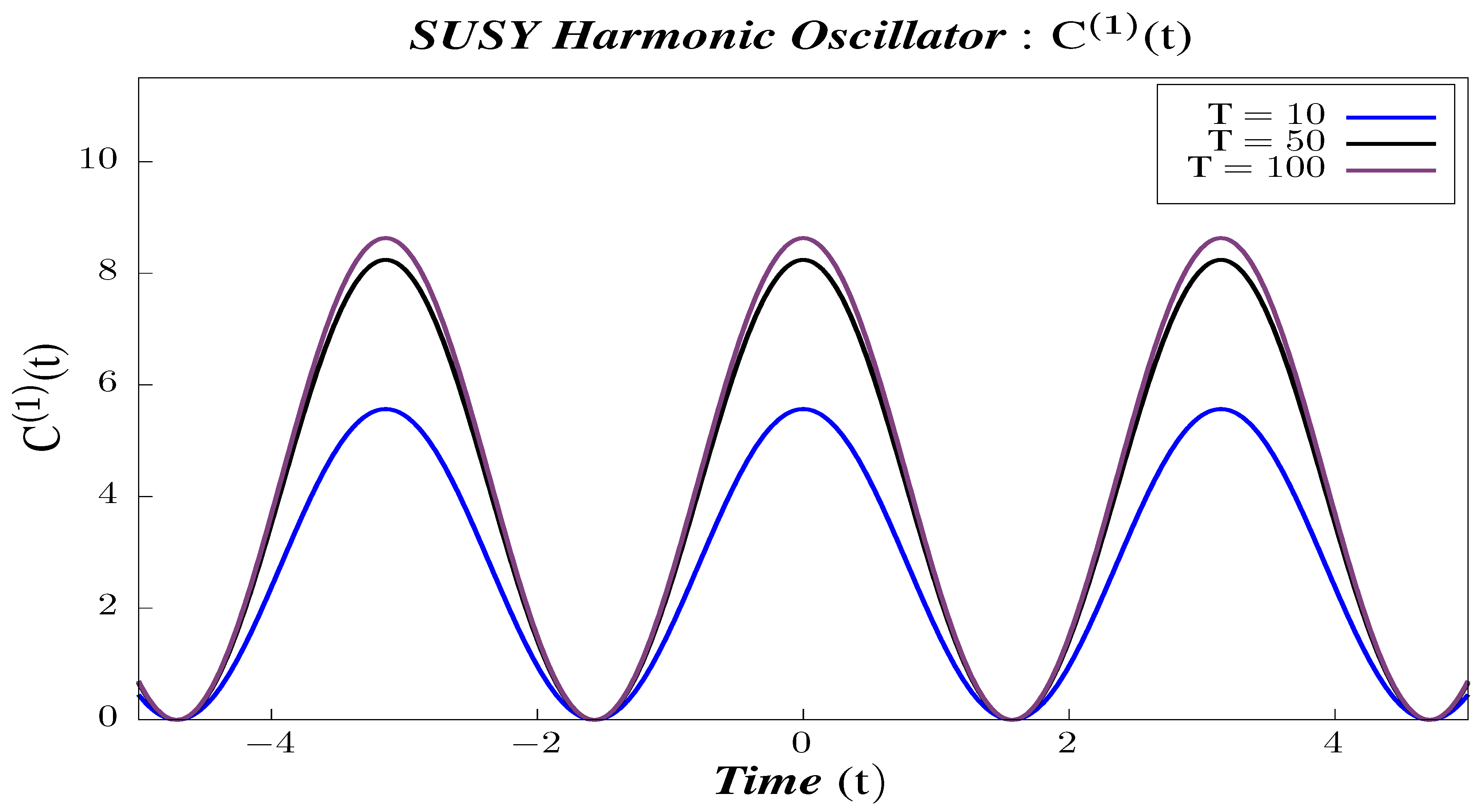
    In Figure 26, Figure 27 and Figure 28, we perform Study B on the 2-point canonical correlators Y ( 1 , 2 , 3 ) ( t 1 , t 2 ) . We observe that the correlators shows periodic behavior for the different chosen values of temperature. We observe that each of the 2-point correlators behave identically with respect to temperature. The amplitude of each of them decreases with increasing temperature. To have a better understanding of the temperature dependence of the 2-point correlators, we plot them with varying temperatures, keeping the time constant.
    -
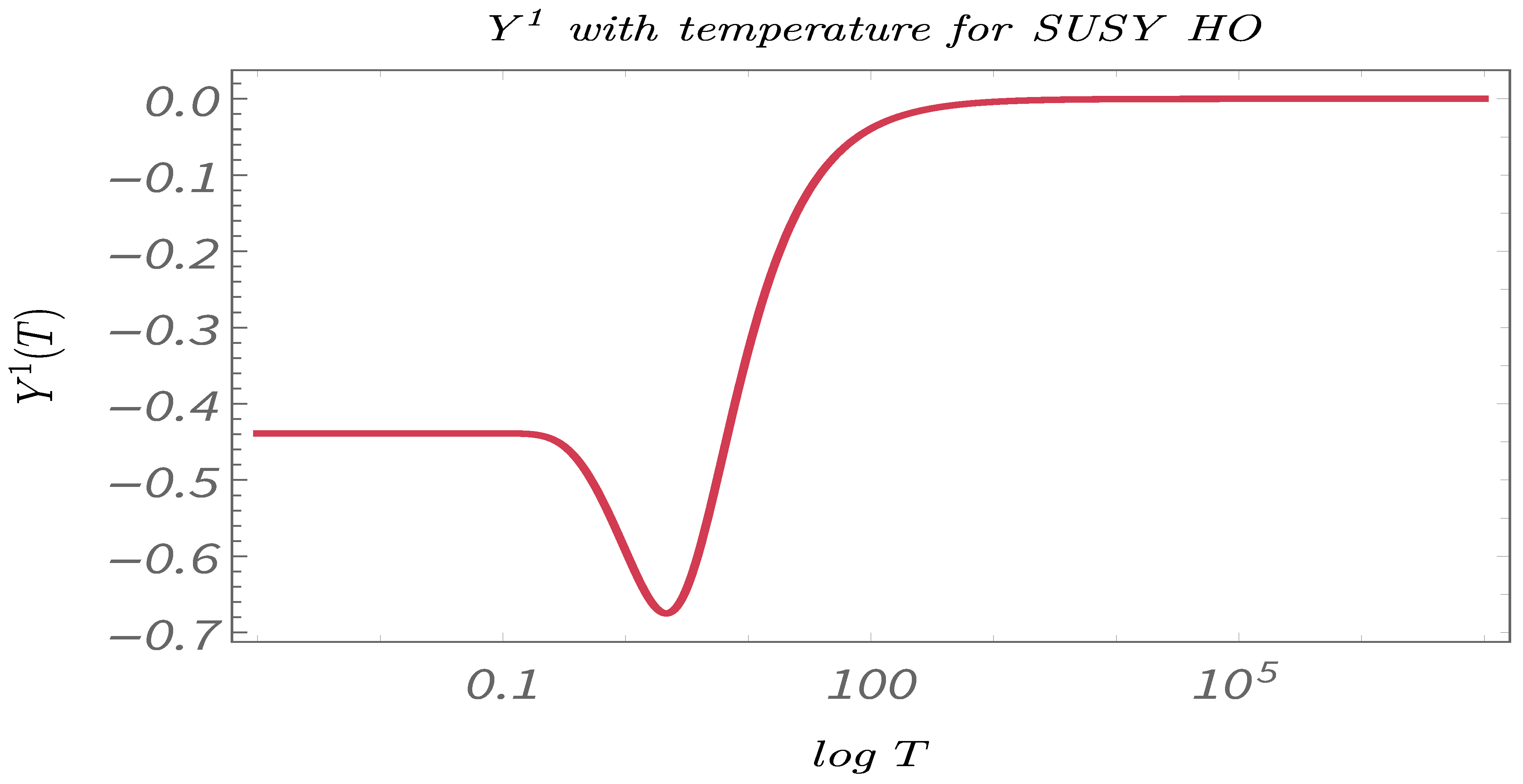
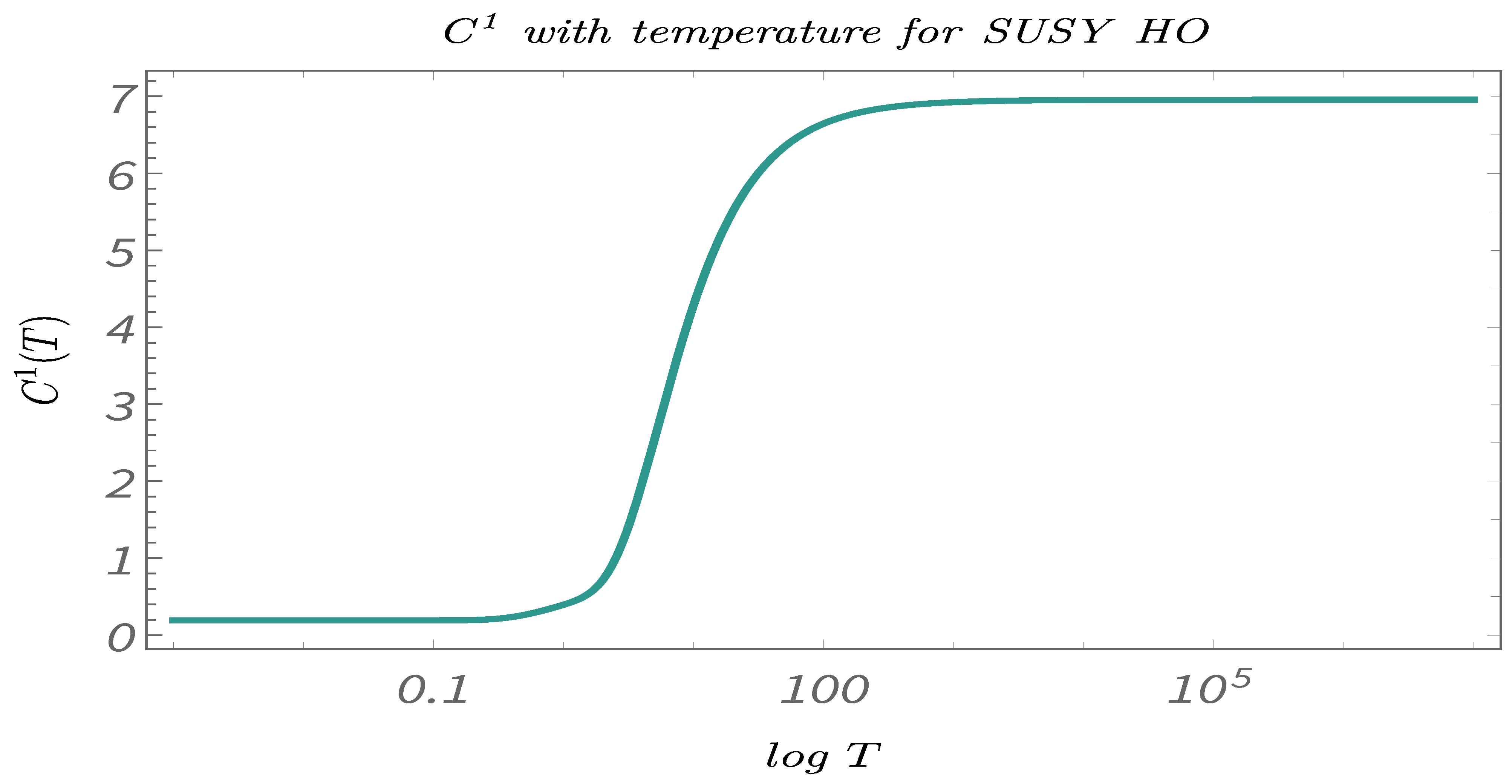
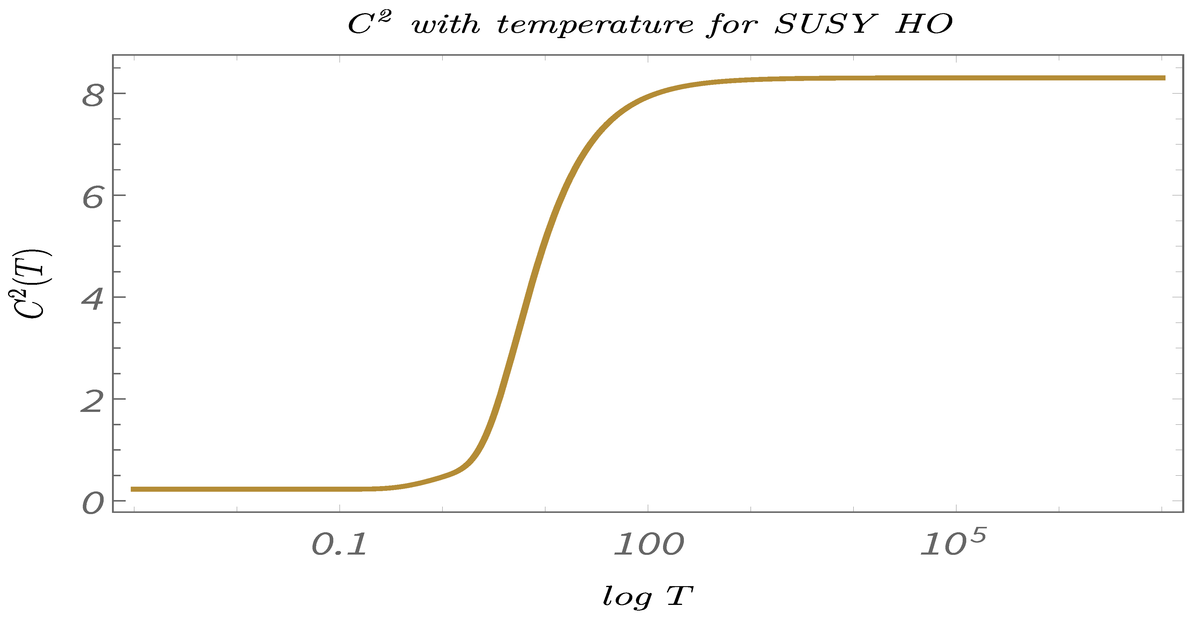
    In Figure 29, Figure 30 and Figure 31, we present the results of performing Study C on 2-point canonical correlators Y ( i ) ( t 1 , t 2 ) . Here, we plot Y ( 1 , 2 , 3 ) ( t 1 , t 2 ) , which are the thermal or canonical correlators corresponding to y m ( 1 , 2 , 3 ) ( t 1 , t 2 ) , respectively, with respect to temperature. It is clearly visible that, for very low temperatures, the canonical correlators are constant. After a certain value of the temperature, the amplitude of the correlator shows a gradual increase. It reaches a maximum for a particular value of the temperature and then decays exponentially to zero.
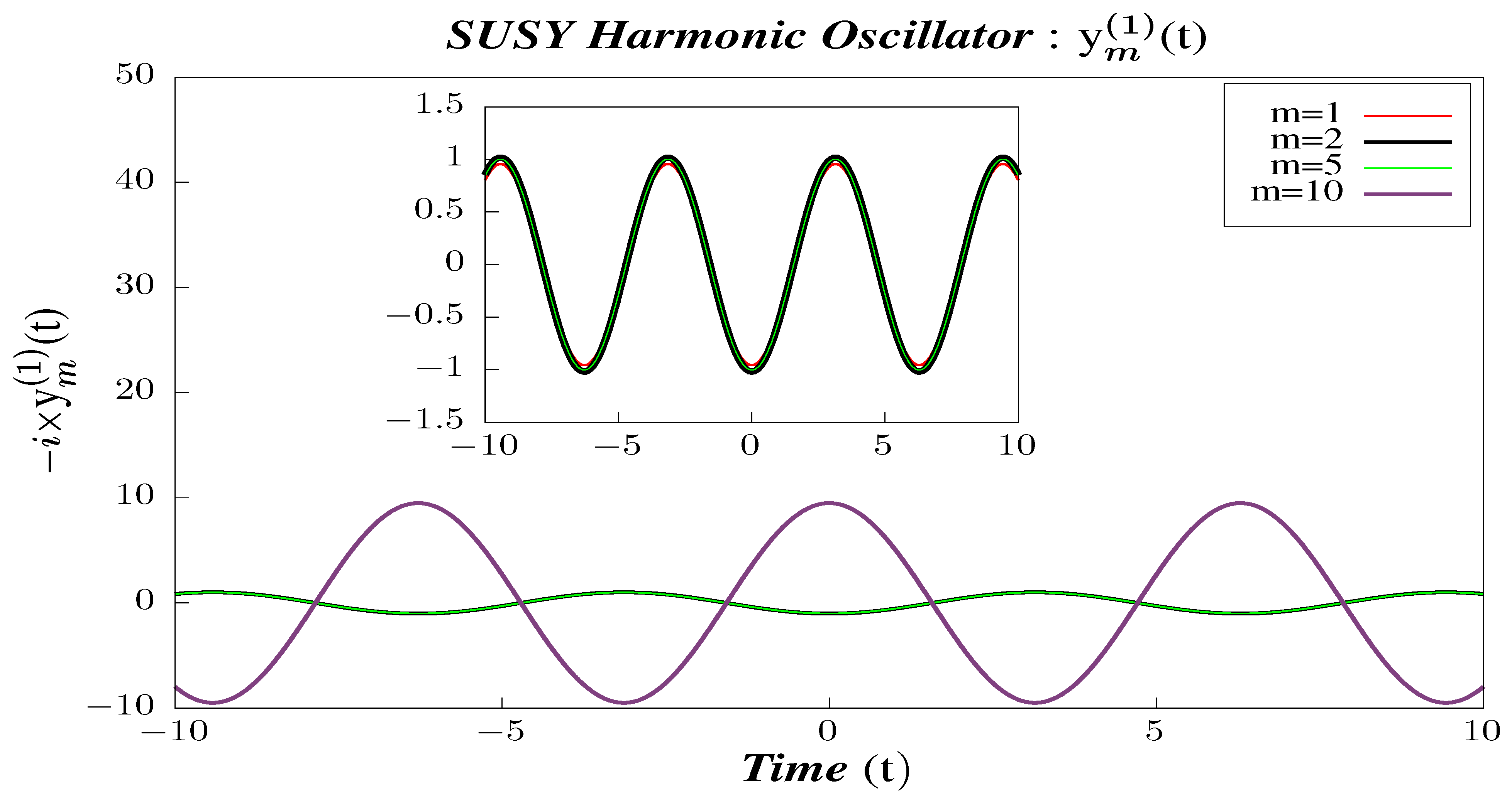
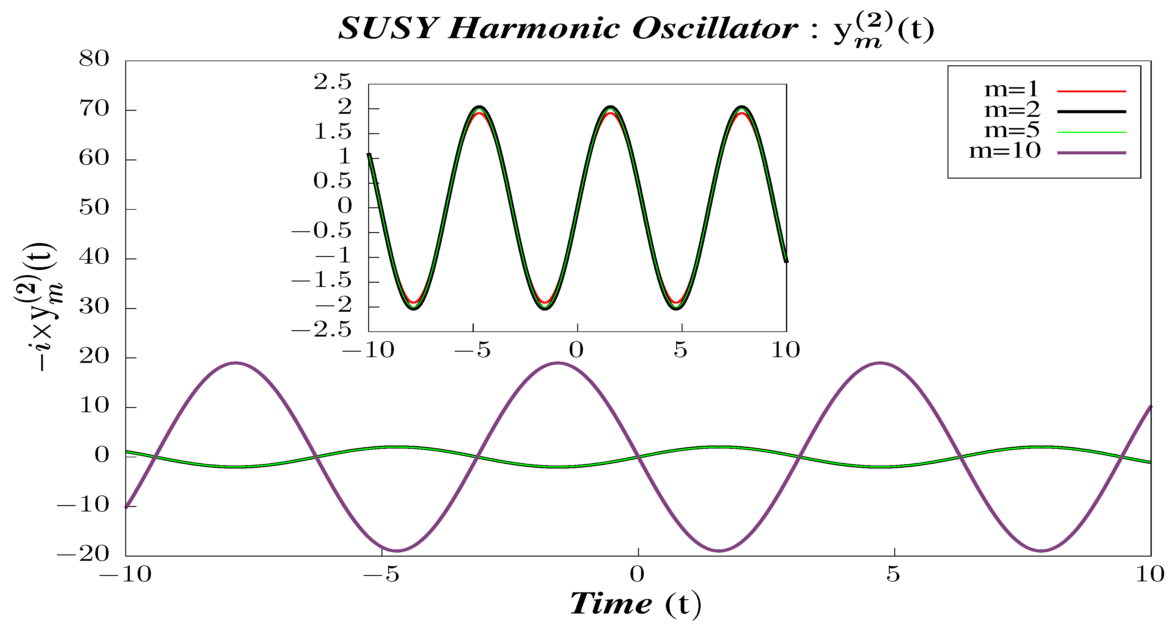
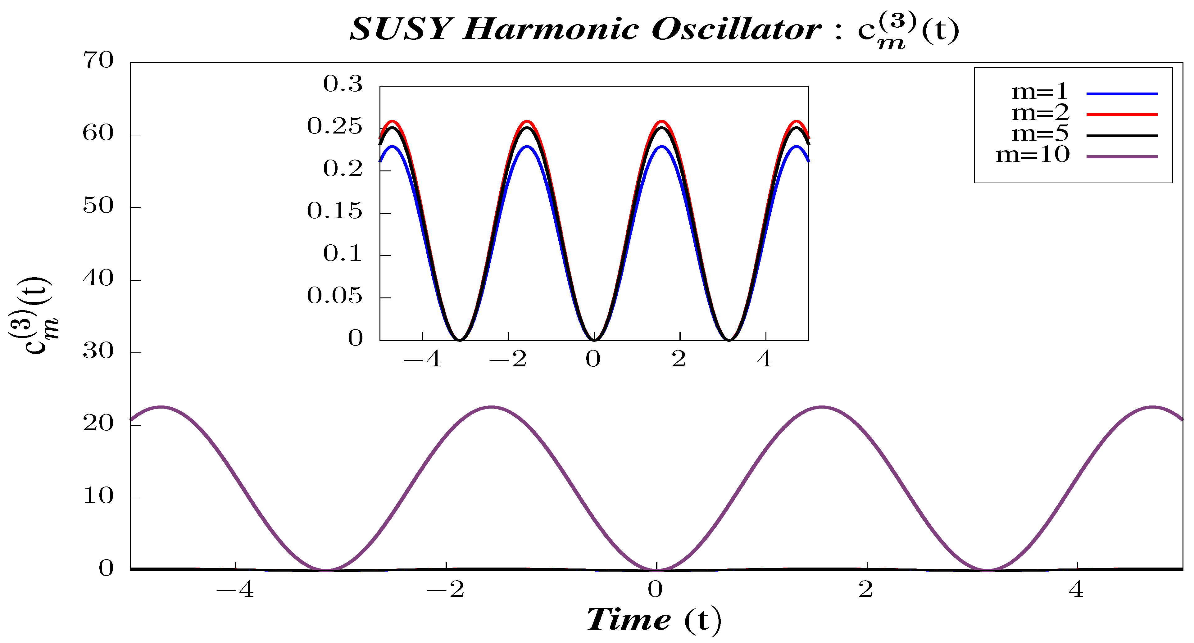
  • In Figure 32, Figure 33 and Figure 34, we perform Study A on the 4-point micro-canonical correlators c m ( 1 , 2 , 3 ) ( t 1 , t 2 ) for Supersymmetric Harmonic Oscillator.
    -
    We observe that the correlators c m ( 1 , 2 , 3 ) ( t 1 , t 2 ) are periodic and that their periodicity does not vary with the state. For the correlator c m ( 1 ) ( t 1 , t 2 ) , the periodicity is roughly half of the corresponding 2-point micro-canonical correlator.
    -
    Other properties of c m ( i ) ( t 1 , t 2 ) are much like y m ( i ) ( t 1 , t 2 ) . We observe a similar change in the amplitude of the correlators with changing m. The scaling of amplitudes in the case of 4-point micro-canonical correlators, c m ( 2 ) ( t 1 , t 2 ) and c m ( 3 ) ( t 1 , t 2 ) is exactly by a factor of 2 than c m ( 1 ) ( t 1 , t 2 ) . This is because, for the 4-point correlators, there is a mass square dependence, unlike the 2-point correlators, which have just mass dependence. The amplitudes of the respective 4-point correlators can also be found to be exactly half of the amplitudes of its 2-point counterpart. This is obvious from the time-dependent functions appearing in the case of Supersymmetric Harmonic oscillator.
    -
    All c m ( i ) ( t 1 , t 2 ) are symmetric about t = 0 , which means that, to these 4-point micro-canonical correlators, it does not matter whether t 1 > t 2 or t 1 < t 2 .
    -
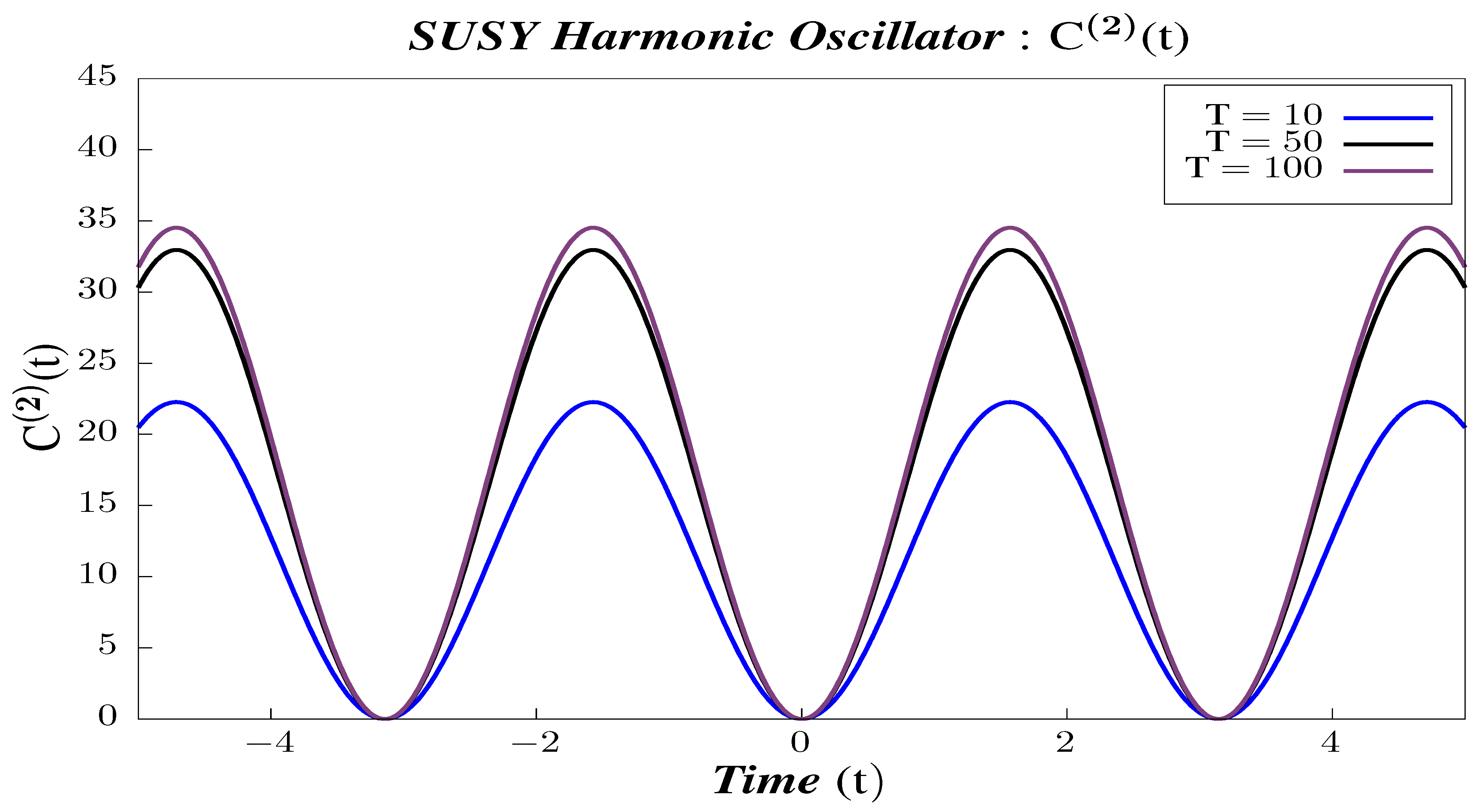
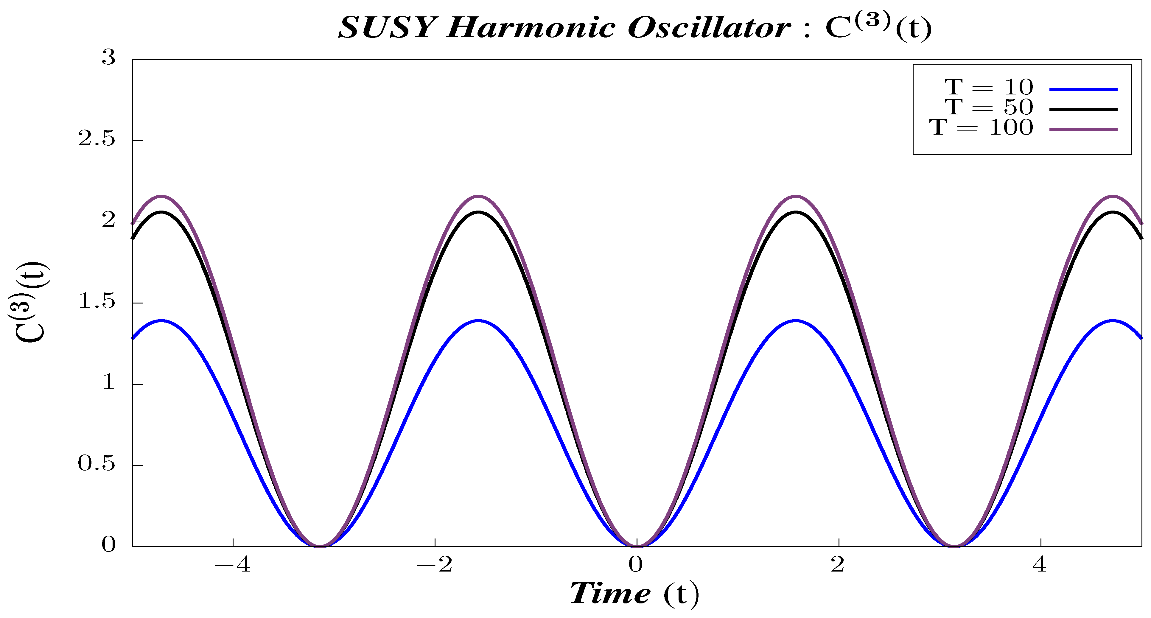
    In Figure 35, Figure 36 and Figure 37, we perform Study B on the 4-point canonical correlators C ( 1 , 2 , 3 ) ( t 1 , t 2 ) . We observe that the correlators shows periodic behavior for the different chosen values of temperature. We observe that each of the 4-point correlators behaves identically with respect to temperature, which is exactly opposite in character from the 2-point canonical correlators. The amplitude of each of them increases with increasing temperature. To have a better understanding of the temperature dependence of the 4-point correlators, we plot them with varying temperature, keeping the time constant.
    -
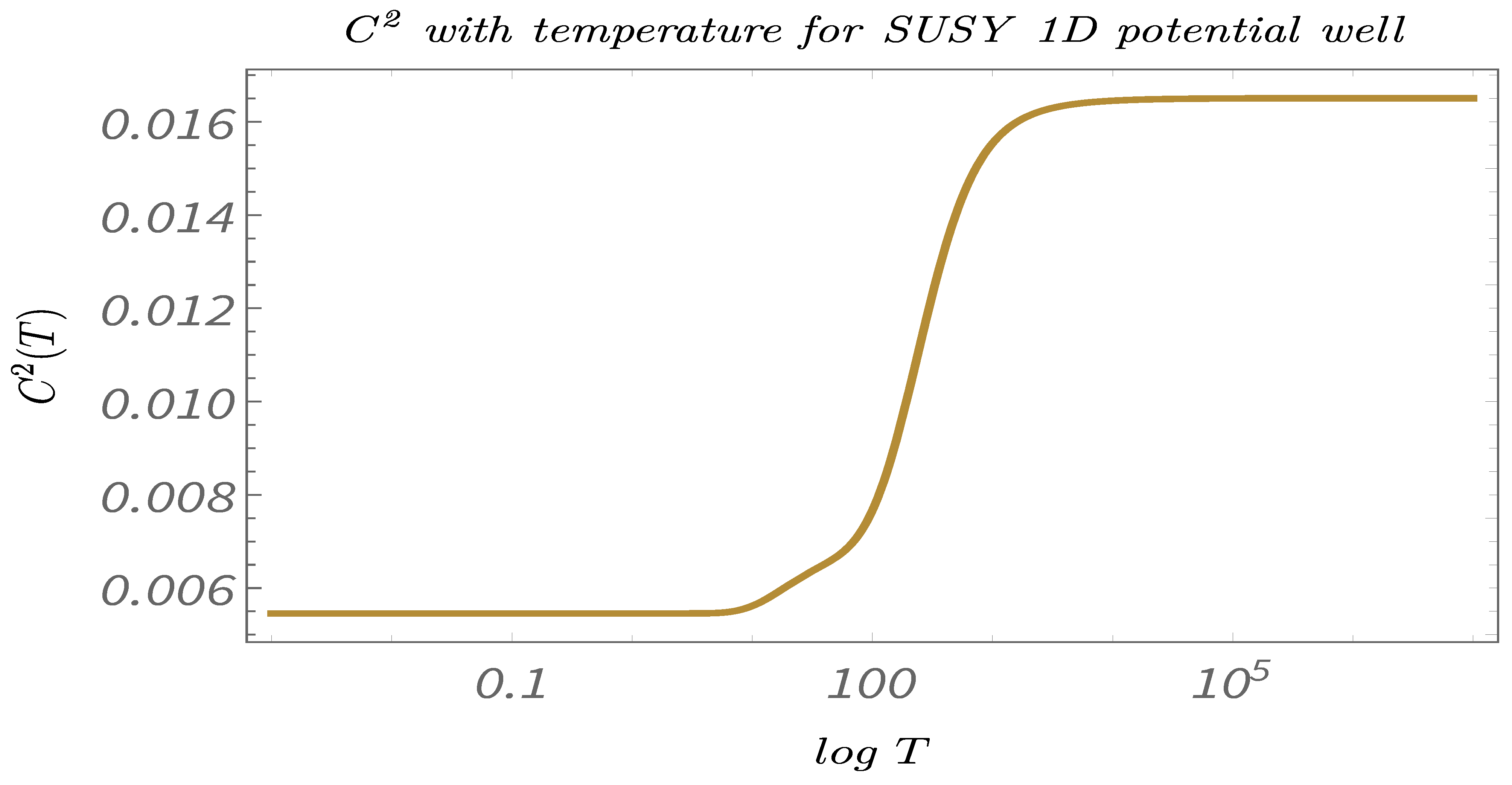
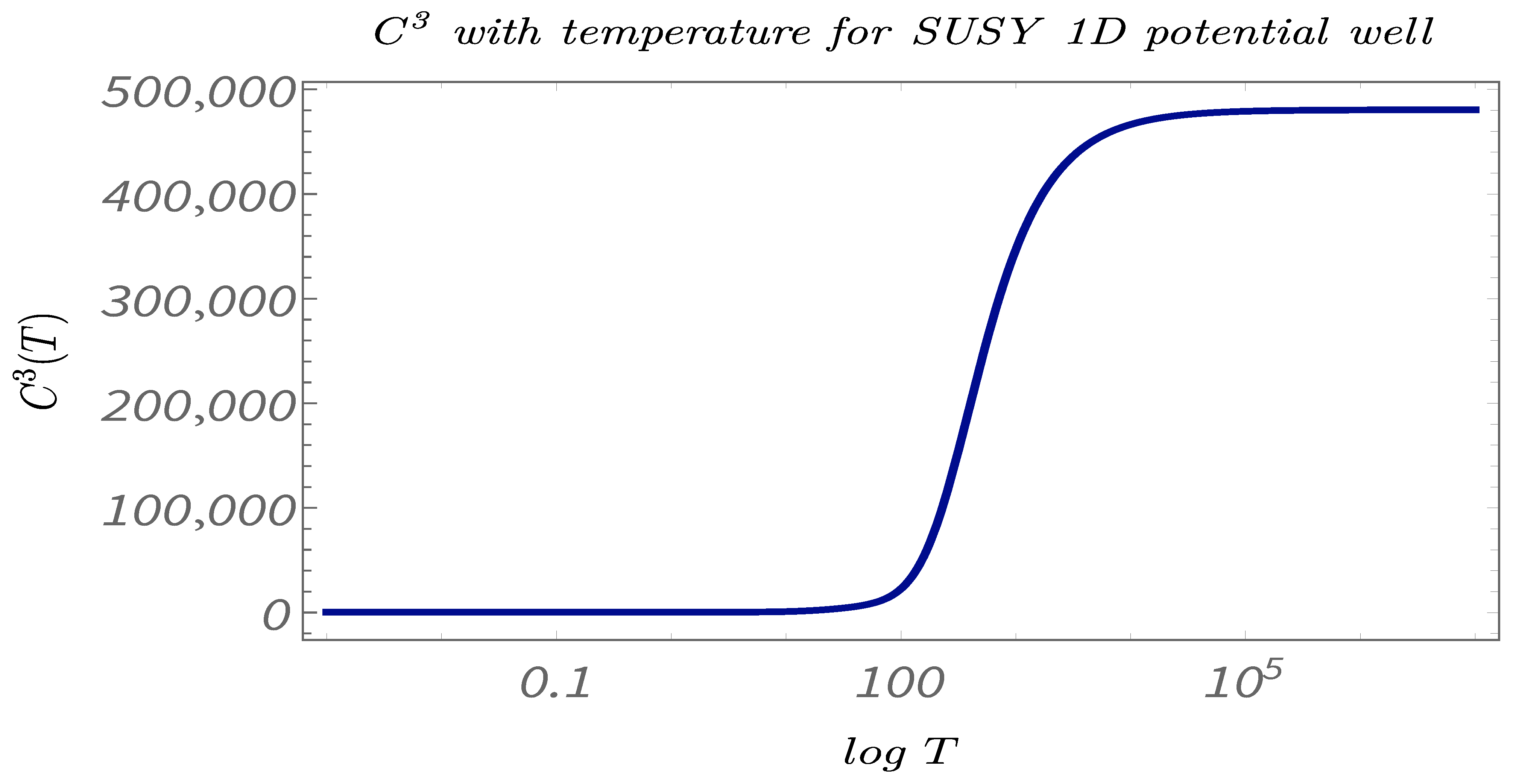
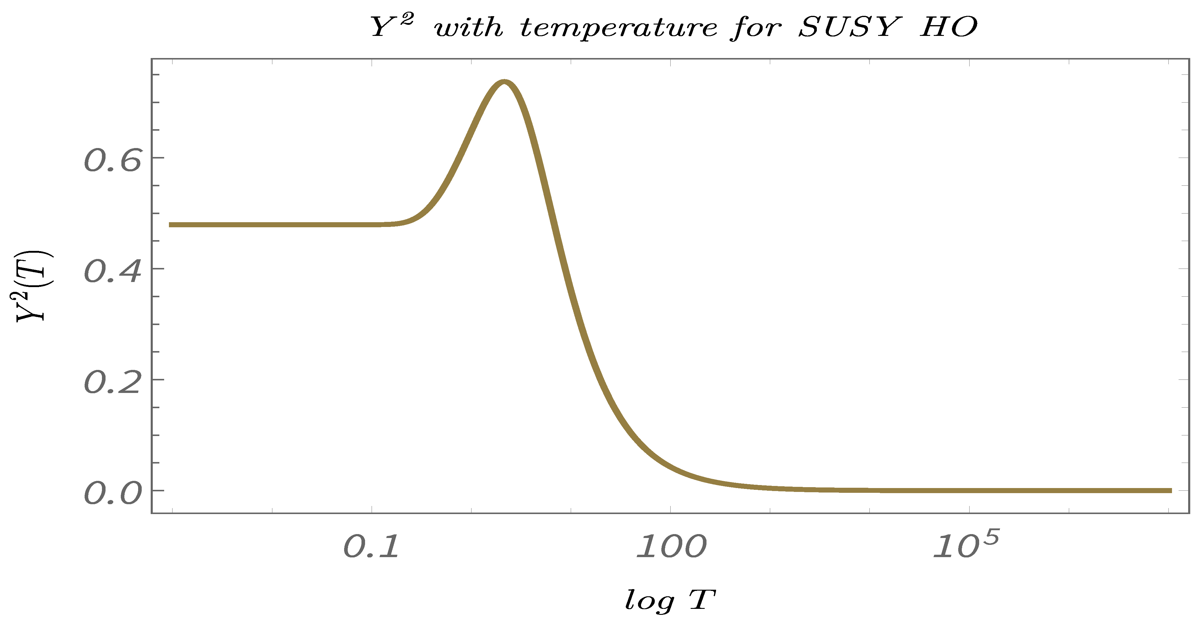
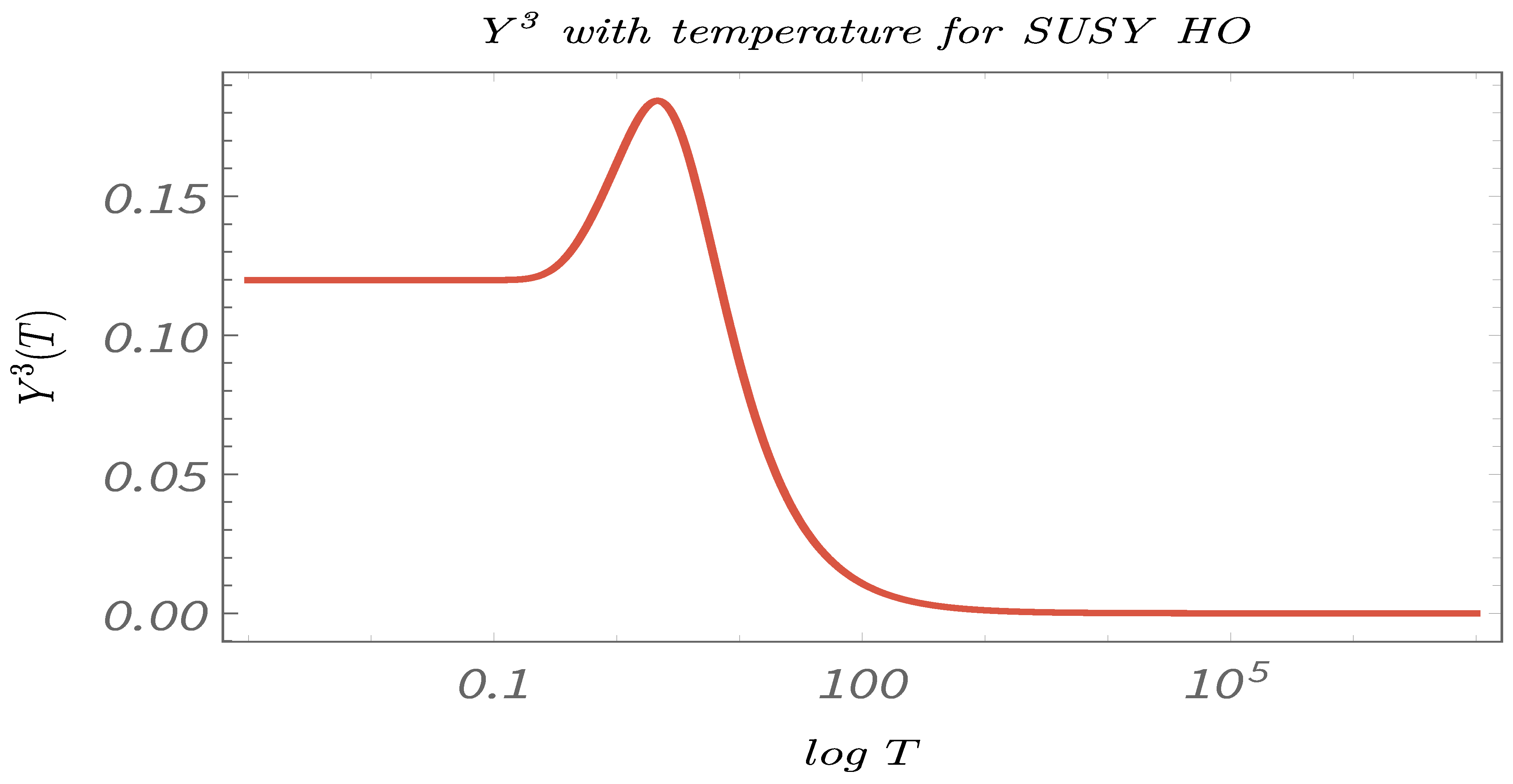
    In Figure 38, Figure 39 and Figure 40, we present the results of performing Study C on 4-point canonical correlators C ( i ) ( t 1 , t 2 ) . Here, we plot C ( 1 , 2 , 3 ) ( t 1 , t 2 ) , which are the thermal or canonical correlators corresponding to y m ( 1 , 2 , 3 ) ( t 1 , t 2 ) , respectively, with respect to temperature. It is clearly visible that, for very low temperatures, the 4-point canonical correlators have negligible amplitudes. After a certain value of the temperature, the amplitude of the correlator starts increasing and, finally, saturates to a finite value.
  • The temperature-dependent plots shows the significance of computing the 4-point and the 2-point correlators to study the phenomenon of quantum randomness for a Supersymmetric quantum mechanical model. From the plots, it can be seen that, for very low temperatures, the 2-point correlators show a certain finite value, whereas the 4-point correlators are almost negligible. On the other hand, at very high temperatures, the 2-point correlators are almost zero, whereas the 4-point correlators shows certain finite value. This suggests that, to understand quantum randomness for a Supersymmetric model at very low temperature, the results from the 4-point correlators can be misleading, and, similarly, at high temperatures, the 2-point correlators might not be an appropriate quantity to study randomness. However, to understand quantum randomness at the mid temperature range, both 2- and 4-point correlators play a significant role. We feel this shows the necessity for computing the 2-point correlators.

12. Conclusions

To summarize, in this work, we have addressed the following issues to study the OTOC in the context of Supersymmetric quantum mechanics:
  • We apply the computational techniques of recently developed methodology of out of time ordered correlators (OTOCs) to study the phenomenon of time disorder averaging for a given quantum statistical ensemble or quantum randomness for two very well known integrable one-dimensional quantum mechanical models viz. Harmonic Oscillator and 1D potential well in the context of one-dimensional Supersymmetric quantum mechanics. We show that, to develop a complete understanding of the underlying randomness in the quantum system, not only the correlators constructed from different operators at different times scales are important but also the correlators, constructed from similar quantum mechanical operators at different time scales, play a pivotal role.
  • We have constructed all the temperature independent micro-canonical and temperature-dependent canonical un-normalized and normalized version of these OTOCs in the eigenstate representation of the Supersymmetric time-independent Hamiltonian of the quantum system and represent all of them in a general model-independent way. From the previous study, it is expected that the OTOCs in the eigenstate representation one should not expect any chaotic behavior, i.e., the exponential growth with respect to the time scale in the correlators. However, one can get a broader knowledge of some other aspects of quantum randomness, which might capture the random behavior in the correlators in terms of non-chaoticity. From our analysis, it is expected that a large class of quantum mechanical models will be covered which provide the signature of quantum mechanical randomness, in general.
  • The explicit calculation of the 4-point correlator C ( 1 ) ( t 1 , t 2 ) , for the Supersymmetric Harmonic Oscillator, shows the significance of the introduction of Supersymmetry within the context of quantum mechanics compared to the framework of quantum mechanics without having any Supersymmetry. Supersymmetry introduces an energy state dependence on the temperature-independent micro-canonical correlators, which usually does not appear in the framework without having Supersymmetry in the quantum mechanics description. Apart from the dependence on the energy states, the canonical correlators have an additional dependence on temperature, which is also a different and notable feature compared to the results obtained from quantum mechanical set up without having Supersymmetry. This energy state and temperature dependence of the correlators differentiates a Supersymmetric and a Non-Supersymmetric Harmonic oscillator [90], though the time dependence in the OTOCs remains same. In addition, particularly for the Supersymmetric Harmonic Oscillator, we have found that the normalized 4-point OTOCs that are made up of same operators at different time scales show exactly the same behavior, which implies they are not independent of each other. However, this statement might not be true for other integrable models. On the other hand, in the un-normalized version of these two correlators, we have found exact same time dependence, but the overall frequency dependent normalization factors will be different, which implies that they are proportional to each other in this case.
  • The classical limit, however, matches with the non-Supersymmetric case apart from a factor of 2, which can be inferred from the fact that, in a Supersymmetric quantum mechanical model, there are two degrees of freedom, one from the original potential and the other associated with the partner potential. The time dependence of the classical and the quantum version of the correlators are exactly identical. However, the temperature dependence observed in the quantum case vanishes for its classical counterpart, which is obviously an important finding from our computation.
  • We observe a similar temperature and state dependence on the correlators for the Supersymmetric 1D Infinite potential well. However, it is interesting to note that Reference [90] also observed this state and temperature dependence for Non-Supersymmetric Infinite potential well. The behavior of the only correlator studied in Reference [90] is exactly identical to what we observe for the Supersymmetric case. The correlator showed increase in the amplitude with increasing state number and higher temperatures, which is exactly what we observe here. Hence, we conclude that introduction of Supersymmetry does not introduce new features in the case of 1D Infinite potential well.
  • The significance of Supersymmetry in 1D potential well, however, can be realized from its classical counterpart, which is markedly different from what is obtained in the non-Supersymmetric case. The classical limit of OTOC for the 1D non-Supersymmetric infinite potential is well independent of time and is merely a constant, whereas, for the Supersymmetric case, there is a non-trivial time dependence, which is obviously a new finding from our computations.
The future prospects of this work are as follows:
  • In this paper, we restricted ourselves in considering only 2- and 4-point correlation functions to study quantum randomness in various Supersymmetric QM models. However, a more generalized approach would be to consider the multipoint correlation functions to have a better understanding about the randomness underlying the system. We have an immediate plan to carry forward the work along this direction very soon.
  • The study of OTOCs can be used to understand quantum randomness in various quantum mechanical models, which are of prime significance in various condensed matter, nuclear, and atomic physics models. Particularly, the time-dependent Hamiltonians we have not studied in this paper are where this eigenstate formalism and related simplification to determine OTOC will not work. In that case, one needs to use the general definition and representation of OTOC in terms of the well known Schwinger Keldysh formalism. We have some future plans on that direction, as well.
  • The other types of correlators defined in this paper can be used to study some of the well understood QM models to have an insight on the lost information of quantum randomness. We are very hopeful that incorporating the study of these additional correlators, which we have defined and evaluated in this paper, can make it possible to capture more broader perspective on time disorder averaging phenomena through quantum randomness, rather than only give insight about quantum mechanical chaos from the temporal growth of the correlators.
  • Very recently, in Reference [110,111,112,113,114], the authors have studied various relevant measures for an entangled open quantum system. The study of OTOCs for such type of entangled systems [115,116,117,118] will be quite relevant for understanding the rtime disorder averaging phenomena and chaos for such an entangled OQS.
  • Last but not least, very recently, we proposed a detailed mechanism and framework, using which one is able to compute the OTOC within the framework of primordial cosmological perturbation theory by making use of the gauge invariant scalar perturbations and its associated canonically conjugate momenta [89], and, finally, found out the chaotic-like behavior in the representative cosmological version of OTOC. However, in that paper, we did not reported anything about the other possible two operators, which we have introduced in this paper. At present, we are working on that direction and very hopeful to get the certain non-trivial features of time disorder averaging, which might have application to explain various cosmologically-relevant phenomena within the evolution history of our universe, which was not explored earlier at all.

Author Contributions

Conceptualization, S.C. (Sayantan Choudhury); methodology, S.C. (Sayantan Choudhury); software, S.C. (Satyaki Chowdhury), N.G.; validation, S.C. (Sayantan Choudhury); formal analysis, S.C. (Sayantan Choudhury), and all other authors of the paper; investigation, S.C. (Sayantan Choudhury); resources, S.C. (Sayantan Choudhury); writing—original draft preparation, S.C. (Sayantan Choudhury), S.C. (Satyaki Chowdhury), N.G.; writing—review and editing, S.C. (Sayantan Choudhury); visualization, S.C. (Sayantan Choudhury); supervision, S.C. (Sayantan Choudhury); project administration, S.C. (Sayantan Choudhury); funding acquisition, S.C. (Sayantan Choudhury). All authors have read and agreed to the published version of the manuscript.

Funding

This research received no external funding.

Institutional Review Board Statement

Not applicable.

Informed Consent Statement

Not applicable.

Data Availability Statement

No data is involved or explicitly used for this work.

Acknowledgments

SC is thankful to Latham Boyle, Robert Myers, Andrew R. Liddle, Douglas Stanford, Alexi Y. Kitaev, Paul Joseph Steinhardt, Martin Bojowald, Eugenio Bianchi, Sudhakar Panda, Soumitra SenGupta, Sumit Ranjan Das, Igor R. Klebanov, Eva Silverstein, Leonardo Senatore, Subhashish Banerjee, Anupam Mazumdar, Savan Kharel for enormous helpful discussions, suggestions, and support. The Post-Doctoral research fellowship of SC is supported by the ERC Consolidator grant 772295 “Qosmology" of Professor Jean-Luc Lehners. SC takes this opportunity to thank sincerely to Jean-Luc Lehners for his constant support and inspiration. SC thanks Latham Boyle for inviting at Perimeter Institute for Theoretical Physics (PITP), Zohar Komargodski for inviting at Simons Center for Geometry and Physics (SCGP), Stony Brook University, Leonardo Senatore for inviting at Institute for Theoretical Physics, Stanford University, Juan Martín Maldacena for inviting at Workshop on Qubits and Spacetime, Institute for Advanced Studies (IAS), Princeton, Paul Joseph Steinhardt for inviting at Department of Physics, Princeton University, Martin Bojowald for inviting at The Institute for Gravitation and the Cosmos (IGC), Department of Physics, Eberly College of Science, Pennsylvania State University (University Park campus), Sudhakar Panda for inviting at School of Physical Sciences, National Institute of Science Education and Research (NISER), Bhubaneswar, Abhishek Chowdhury for inviting at Department of Physics, Indian Institute of Technology (IIT), Bhubaneswar, Anjan Sarkar for inviting at Department of Astrophysics, Raman Research Institute, Bengaluru, Aninda Sinha and Banibrata Mukhopadhyay for inviting at Center for High Energy Physics (CHEP) and Department of Astronomy and Astrophysics, Indian Institute of Science, Bengaluru, Uma Shankar for inviting at Department of Physics, Indian Institute of Technology (IIT), Bombay, Shiraz Minwalla for inviting at Department of Theoretical Physics, Tata Institute of Fundamental Research, Mumbai, Abhishek Mahapatra for inviting at National Institute of Technology (NIT), Rourkela, for official academic visit where the work was done partially. Part of this work was presented as a talk, titled “Cosmology from Condensed Matter Physics: A study of out-of-equilibrium physics” and “ Cosmology Meets Condensed Matter Physics” at Perimeter Institute for Theoretical Physics (PITP) (See the link: http://pirsa.org/19110117/), Simons Center for Geometry and Physics (SCGP), Stony Brook University (See the link: http://scgp.stonybrook.edu/videoportal/video.php?id=4358), Department of Physics, Princeton University, The Institute for Gravitation and the Cosmos (IGC), Department of Physics, Eberly College of Science, Pennsylvania State University (University Park campus), workshop on “Advances in Astroparticle Physics and Cosmology, AAPCOS-2020” at Saha Institute of Nuclear Physics, Kolkata on the occasion of the 100 years of Saha Ionisation Equation by Meghnad Saha, Department of Physics, Scottish Church College, Kolkata, School of Physical Sciences, National Insitute of Science Education and Research (NISER), Bhubaneswar, Department of Physics, Indian Institute of Technology (IIT), Bhubaneswar, Department of Astrophysics, Raman Research Institute, Bengaluru, Center for High Energy Physics (CHEP), Indian Institute of Science, Bengaluru, Department of Physics, Indian Institute of Technology (IIT), Bombay, National Institute of Technology (NIT), Rourkela. SC would like to thank Quantum Gravity and Unified Theory and Theoretical Cosmology Group, Max Planck Institute for Gravitational Physics, Albert Einstein Institute (AEI), Perimeter Institute for Theoretical Physics (PITP), Simons Center for Geometry and Physics (SCGP), Stony Brook University, Institute for Theoretical Physics, Stanford University, The Institute for Gravitation and the Cosmos (IGC), Department of Physics, Eberly College of Science, Pennsylvania State University (University Park campus), School of Physical Sciences, National Insitute of Science Education and Research (NISER), Bhubaneswar, Department of Astrophysics, Raman Research Institute, Bengaluru, Department of Physics, Indian Institute of Technology (IIT), Bombay, Quantum Space-time Group (Earlier known as String Theory and Mathematical Physics Group), Department of Theoretical Physics, Tata Institute of Fundamental Research, Mumbai and National Institute of Technology (NIT), Rourkela for providing financial support for the academic visits at Canada, U.S.A. and India. SC would like to thank the natural beauty of Prague, Dresden, Hamburg, Leipzig, Potsdam, Berlin, Mumbai, Bangalore, Kolkata, Bhubaneswar, which inspired us to work very hard during the weekend trips and various academic visits. Particularly, SC wants to give a separate credit to all the members of the EINSTEIN KAFFEE Berlin Alexanderplatz for providing work friendly environment, good espresso shots, and cookies, which helped to write the most of the part of the paper in that coffee shop. SC also thanks all the members of our newly-formed virtual international non-profit consortium “Quantum Structures of the Space-Time & Matter" (QASTM) for elaborative discussions. SC also would like to thank all the speakers of QASTM zoominar series from different parts of the world (For the uploaded YouTube link, look at: https://www.youtube.com/playlist?list=PLzW8AJcryManrTsG-4U4z9ip1J1dWoNgd.) for supporting my research forum by giving outstanding lectures and their valuable time during this COVID pandemic time. KYB, SC (Satyaki), NG, RND, AM, GDP, SP would like to thank IISC Bangalore, NISER Bhubaneswar, IISER Mohali, IIT Bombay, University of Waterloo, and IIT Indore, respectively, for providing fellowships. We would like to dedicate this work for the people those who are helping us to fight against COVID-19 pandemic across the globe. Last but not least, we would like to acknowledge our debt to the people belonging to the various part of the world for their generous and steady support for research in natural sciences.

Conflicts of Interest

The authors declare no conflict of interest.

Appendix A. Derivation of the Normalization Factors for the Supersymmetric HO

To normalize the obtained OTOC, we divide it by the thermal average of the dynamical variables considered in calculating the OTOC.
x ( t 1 ) x ( t 1 ) β = 1 Z Tr ( e β H x ( t 1 ) x ( t 1 ) ) = 1 Z n e β n ω Ψ n | p ( t 1 ) p ( t 1 ) | Ψ n .
Now, keep in mind that the ground state is only bosonic, whereas all the other eigenstates have a fermionic part associated with it. Hence, separating the ground state from the other states, the above equation can be written as
x ( t 1 ) x ( t 1 ) β = 1 Z ψ 0 | x ( t 1 ) x ( t 1 ) | ψ 0 + n > 0 e β n ω ψ n | x ( t 1 ) x ( t 1 ) | ψ n = 1 Z k [ ψ 0 | x ( t 1 ) | ψ k ψ k | x ( t 1 ) | ψ 0 Term A + n > 0 e β n ω ψ n | x ( t 1 ) | ψ k ψ k | x ( t 1 ) | ψ n Term B ] .
Now, we are going to explicitly show the calculation of term A and term B. Expanding the position operators using the Heisenberg picture for the evolution of operators:
Term A = k ψ 0 | x ( t 1 ) | ψ k ψ k | x ( t 1 ) | ψ 0 = 1 2 k e i k ω t 1 x 0 k B e i k ω t 1 x k 0 B = 1 2 k x 0 k B x k 0 B = 1 4 ω .
Term B = n > 0 e β n ω k ψ n | x ( t 1 ) | ψ k ψ k | x ( t 1 ) | ψ n = n > 0 e β n ω ψ n | x ( t 1 ) | ψ 0 ψ 0 | x ( t 1 ) | ψ n + n > 0 e β n ω k > 0 ψ n | x ( t 1 ) | ψ k ψ k | x ( t 1 ) | ψ n = 1 2 n > 0 e β n ω e i n ω t 1 x n 0 e i n ω t 1 x 0 n + n > 0 k > 0 x n k ( t 1 ) x k n ( t 1 ) = e β ω 4 ω + 1 4 ω n > 0 e β n ω 2 n + n ( n + 1 ) + n ( n 1 ) .
x ( t 1 ) x ( t 1 ) β = 1 4 Z ω 1 + e β ω + n > 0 e β E n [ 2 n + n ( n + 1 ) + n ( n 1 ) ] .
A similar calculation is carried out for the thermal average of the product of the momentum operators.
p ( t 2 ) p ( t 2 ) β = 1 Z Tr ( e β H p ( t 2 ) p ( t 2 ) ) = 1 Z n e β n ω Ψ n | p ( t 2 ) p ( t 2 ) | Ψ n .
Now, keep in mind that the ground state is only bosonic, whereas all the other eigenstates have a fermionic part associated with it. Hence, separating the ground state from the other states, the above equation can be written as
p ( t 2 ) p ( t 2 ) β = 1 Z ψ 0 | p ( t 2 ) p ( t 2 ) | ψ 0 + n > 0 ψ n | p ( t 2 ) p ( t 2 ) | ψ n = 1 Z k [ ψ 0 | p ( t 2 ) | ψ k ψ k | p ( t 2 ) | ψ 0 Term A + n > 0 ψ n | p ( t 2 ) | ψ k ψ k | p ( t 2 ) | ψ n Term B ] .
Now, we are going to explicitly show the calculation of term A and term B. Expanding the position operators using the Heisenberg picture for the evolution of operators:
Term A = k ψ 0 | p ( t 2 ) | ψ k ψ k | p ( t 2 ) | ψ 0 = 1 2 k e i E 0 k t 2 p 0 k B e i E k 0 t 2 p k 0 B = 1 2 k p 0 k B p k 0 B = ω 4 .
Term B = n > 0 e β E n k ψ n | p ( t 2 ) | ψ k ψ k | p ( t 2 ) | ψ n = n > 0 e β E n ψ n | p ( t 2 ) | ψ 0 ψ 0 | p ( t 2 ) | ψ n + n > 0 k > 0 ψ n | p ( t 2 ) | ψ k ψ k | p ( t 2 ) | ψ n = 1 2 n > 0 e β E n e i E n 0 t 2 p n 0 e i E 0 n t 2 p 0 n + n > 0 k > 0 p n k ( t 2 ) p k n ( t 2 ) = ω e β ω 4 + ω 4 n > 0 e β E n 2 n + n ( n + 1 ) + n ( n 1 ) .
p ( t 2 ) p ( t 2 ) β = ω 4 Z 1 + e β ω + n > 0 e β E n 2 n + n ( n + 1 ) + n ( n 1 ) .

Appendix B. Poisson Bracket Relation for the Supersymmetric Partner Potential Associated with the 1D Infinite Well Potential

For calculating the Poisson Bracket { x 2 ( t 1 ) , p 2 ( t 2 ) } , we need the partial derivaties of the dynamical variables characterising the partner hamiltonian with respect to their initial values. For the partner potential associated with the 1D box, it can be seen from Equations (261) and (262) that the partial derivatives of the classical variables with respect to its initial value will not be trivial and will depend on the initial value chosen. For the sake of convenience, we introduce some symbols in this section. We denote the partial derivative of position with respect to its initial value with the symbol O 1 O 2 , i.e.,
x 2 ( t ) x 2 ( 0 ) = ( 1 ) n O 1 O 2 .
where the symbols O 1 and O 2 have the following expressions:
O 1 = 1 + 4 π 4 cos ( sin 1 ( α ) t β ) sin ( π x 2 ( 0 ) ) ( p 2 ( 0 ) 2 + 4 p 2 ( 0 ) 2 π 4 + 16 π 8 cot 4 ( π x 2 ( 0 ) ) + 8 π 4 cot 2 ( π x 2 ( 0 ) ) ( p 2 ( 0 ) 2 2 π 4 2 π 4 cosec 2 ( π x 2 ( 0 ) ) ) 16 π 8 cot 3 ( π x 2 ( 0 ) ) t c cosec 3 ( π x 2 ( 0 ) ) p 2 ( 0 ) 2 sin 2 ( π x 2 ( 0 ) ) c 4 π 4 t cot ( π x 2 ( 0 ) ) c 3 cosec 5 ( π x 2 ( 0 ) ) [ p 2 ( 0 ) 2 sin 2 ( π x 2 ( 0 ) ) c ] 3 / 2 ) .
O 2 = c 2 p 2 ( 0 ) 2 sin ( π x 2 ( 0 ) ) c η ( t ) .
Similarly, for the partial derivative of x 2 ( t ) with p 2 ( 0 ) , we get
x 2 ( t ) p 2 ( 0 ) = p 2 ( 0 ) 1 + 4 π 4 cos [ sin 1 ( α ) t β ] ( 4 π 4 c o s ( π x 2 ( 0 ) ) + c 3 t ) p 2 ( 0 ) 2 sin 2 ( π x 2 ( 0 ) ) c π c 3 β p 2 ( 0 ) 2 sin 2 ( π x 2 ( 0 ) ) c η ( t ) ,
where the symbols α , β , and η ( t ) used in the above equations have the following expressions.
α = cos ( π x 2 ( 0 ) ) p 2 ( 0 ) 2 + 4 π 4 cot 2 ( π x 2 ( 0 ) ) p 2 ( 0 ) 2 + 4 π 4 + 4 π 4 cot 2 ( π x 2 ( 0 ) ) , β = p 2 ( 0 ) 2 + 4 π 4 + 4 π 4 cot 2 ( π x 2 ( 0 ) ) , η ( t ) = ( 1 ( 1 + 4 π 4 ) sin 2 [ sin 1 ( α ) t β ] ) .
The partial derivative of the momentum associated with the partner potential wrt its initial position and the momentum are now explicitly evaluated. The partial derivative of the momentum wrt the initial position is given by
p 2 ( t ) x 2 ( 0 ) = 4 π 5 ( cot ( π x 2 ( 0 ) ) cosec 2 ( π x 2 ( 0 ) ) + Y 1 Y 2 Y 3 Y 4 ) c 2 4 π 4 ( 1 + 4 π 4 ) sin 2 [ sin 1 ( α ) β t ] η ( t ) .
where the symbols Y 1 , Y 2 , Y 3 , Y 4 used in the above equations refers to the following:
Y 1 = ( 1 + 4 π 4 ) 2 cos [ sin 1 ( α ) β t ] sin ( π x 2 ( 0 ) ) ( p 2 ( 0 ) 4 + 4 p 2 ( 0 ) 2 π 4 + 16 π 8 cot 4 ( π x 2 ( 0 ) ) + 8 π 4 cot 2 ( π x 2 ( 0 ) ) ( p 2 ( 0 ) 2 + 2 π 4 2 π 4 cosec 2 ( π x 2 ( 0 ) ) ) 16 π 8 t cot 2 ( π x 2 ( 0 ) ) c cosec 3 ( π x 2 ( 0 ) ) p 2 ( 0 ) 2 sin 2 ( π x 2 ( 0 ) ) c 2 4 π 4 t cot ( π x 2 ( 0 ) ) c 3 cosec 5 ( π x 2 ( 0 ) ) ( p 2 ( 0 ) 2 sin 2 ( π x 2 ( 0 ) ) c 2 ) 3 / 2 ) sin 3 [ sin 1 ( α ) t β ] ,
Y 2 = c 3 β p 2 ( 0 ) 2 sin 2 ( π x 2 ( 0 ) ) c 2 ( 1 + ( 1 + 4 π 4 ) sin 2 [ sin 1 ( α ) β t ] ) 2 ,
Y 3 = ( 1 + 4 π 4 ) sin ( π x 2 ( 0 ) ) ( p 2 ( 0 ) 4 + 4 p 2 ( 0 ) 2 π 4 + 16 π 8 cot 4 ( π x 2 ( 0 ) ) + 8 π 4 cot 2 ( π x 2 ( 0 ) ) ( p 2 ( 0 ) 2 + 2 π 4 2 π 4 cosec 2 ( π x 2 ( 0 ) ) ) 16 π 8 t cot 2 ( π x 2 ( 0 ) ) c cosec 3 ( π x ( 0 ) ) p ( 0 ) 2 sin 2 ( π x 2 ( 0 ) ) c 2 4 π 4 t cot ( π x 2 ( 0 ) ) c 3 cosec 5 ( π x 2 ( 0 ) ) ( p 2 ( 0 ) 2 sin 2 ( π x 2 ( 0 ) ) c 2 ) 3 / 2 sin [ 2 sin 1 ( α ) 2 β t ] ) ,
Y 4 = 2 c 3 β p 2 ( 0 ) 2 sin 2 ( π x 2 ( 0 ) ) c 2 ( 1 + ( 1 + 4 π 4 ) sin 2 [ sin 1 ( α ) β t ] ) .
The partial derivative of the momentum wrt the initial momentum is given by
p 2 ( t ) p 2 ( 0 ) = ( 2 p 2 ( 0 ) + Z 1 Z 2 Z 3 Z 4 ) 2 c 2 + 4 π 4 ( 1 + 4 π 4 ) sin 2 [ sin 1 ( α ) β t ] 1 + ( 1 + 4 π 4 ) sin 2 [ sin 1 ( α ) β t ] ,
where the symbols Z 1 , Z 2 , Z 3 , Z 4 represent the following expressions:
Z 1 = 8 p 2 ( 0 ) π 4 ( 1 + 4 π 4 ) 2 cos [ sin 1 ( α ) β t ] ( 4 π 4 cos ( π x 2 ( 0 ) ) + c 3 t p 2 ( 0 ) 2 sin 2 ( π x 2 ( 0 ) ) c 2 ) sin 3 [ sin 1 ( α ) β t ] ,
Z 2 = c 3 β p 2 ( 0 ) 2 sin 2 ( π x 2 ( 0 ) ) c 2 ( 1 + ( 1 + 4 π 4 ) sin 2 [ sin 1 ( α ) β t ] ) ,
Z 3 = 4 p 2 ( 0 ) π 4 ( 1 + 4 π 4 ) ( 4 π 4 cos ( π x 2 ( 0 ) ) + 2 t c 3 · p 2 ( 0 ) 2 sin 2 ( π x 2 ( 0 ) ) p 2 ( 0 ) 2 + 4 π 4 + ( p 2 ( 0 ) 2 + 4 π 4 ) cos ( 2 π x 2 ( 0 ) ) ) ,
Z 4 = c 3 β p 2 ( 0 ) 2 sin 2 ( π x 2 ( 0 ) ) c ( 1 + ( 1 + 4 π 4 ) sin 2 [ sin 1 ( α ) β t ] ) .
In a similar way, for the Poisson Bracket involving the position and momentum variables at different times, we denote it by X 2 P 2 , for the sake of convenience, i.e.,
{ x 2 ( t 1 ) , p 2 ( t 2 ) } = ( 1 ) n X 2 Q 2 ,
where X 2 and Q 2 can be explicitly evaluated to have the following expressions:
X 2 = p 2 ( 0 ) 1 + 4 π 4 [ 3 p 2 ( 0 ) 4 + 20 p 2 ( 0 ) 2 π 4 + 64 π 8 4 ( p 2 ( 0 ) 4 + 4 p ( 0 ) 2 π 4 16 π 8 ) cos ( 2 π x ( 0 ) ) + ( p 2 ( 0 ) 2 4 p 2 ( 0 ) 2 π 4 ) cos ( 4 π x ( 0 ) ) ] cos [ sin 1 α t 1 γ 2 ] cosec 3 ( π x 2 ( 0 ) ) ( 3 γ 2 4 2 π 4 γ + 24 2 π 8 γ + ( 1 + 4 π 4 ) 2 cos [ 4 sin 1 ( α ) 2 2 t 2 γ ] γ 2 2 2 ( 1 + 16 π 8 ) cos [ 2 sin 1 ( α ) 2 t 2 γ ] 16 π 4 t 1 sin [ 2 sin 1 ( α ) 2 t 2 γ ] 64 π 8 t 1 sin [ 2 sin 1 ( α ) 2 t 2 γ ] + 16 π 4 t 2 sin [ 2 sin 1 ( α ) 2 t 2 γ ] + 64 π 8 t 2 sin [ 2 sin 1 ( α ) 2 t 2 γ ] ) . Q 2 = 64 c 2 β 2 p 2 ( 0 ) sin ( π x 2 ( 0 ) ) η ( t 1 ) ( η ( t 2 ) ) 2 c 2 4 π 4 ( 1 + 4 π 4 ) sin 2 [ sin 1 ( α ) t 2 β ] η ( t 2 ) .
The symbol γ used in the above equations denotes the following expression:
γ = p 2 ( 0 ) 2 + 8 π 4 p 2 ( 0 ) 2 cos ( 2 π x 2 ( 0 ) ) cosec ( π x 2 ( 0 ) ) .
The Poisson Bracket of the momentum at different times is symbolically denoted by { p 2 ( t 1 ) , p 2 ( t 2 ) } = P 1 / P 2 , where P 1 and P 2 represent the following expressions:
P 1 = 2 p ( 0 ) π 4 ( 1 + 4 π 4 ) sin ( π x ( 0 ) ) ( 1 4 ( 1 4 π 4 + ( 1 + 4 π 4 ) cos [ 2 sin 1 ( α ) 2 β t 1 ] ) ) 2 β sin [ 2 sin 1 ( α ) 2 t 2 β ] + sin [ 2 sin 1 ( α ) 2 t 1 β ] ( 1 4 ( 1 4 π 4 + ( 1 + 4 π 4 ) cos [ 2 sin 1 ( α ) 2 t 2 β ] ) 2 β 2 π 4 ( 1 + 4 π 4 ) ( t 1 t 2 ) sin [ 2 sin 1 ( α ) 2 t 2 β ] ) ,
P 2 = { p ( 0 ) sin ( π x ( 0 ) ) ( ( 1 + 4 π 4 ) sin 2 [ sin 1 ( α ) t 1 β ] 1 ) 2 × c 2 + 4 π 4 ( 1 + 4 π 4 ) sin 2 [ sin 1 ( α ) t 1 β ] ( 1 + 4 π 4 ) sin 2 [ sin 1 ( α ) t 1 β ] 1 } × ( ( 1 + 4 π 4 ) sin 2 [ sin 1 ( α ) t 2 β ] 1 ) 2 × c 2 + 4 π 4 ( 1 + 4 π 4 ) sin 2 [ sin 1 ( α ) t 2 β ] ( 1 + 4 π 4 ) sin 2 [ sin 1 ( α ) t 2 β ] 1 .

Appendix C. Derivation of the Eigenstate Representation of the Correlators

We provide a detailed derivation of the eigenstate representation of the various 2-point and the 4-point correlators that we intend to calculate for various Supersymmetric quantum mechanical models.

Appendix C.1. Representation of 2-point Correlator: Y ( 1 ) ( t 1 , t 2 )

We have the correlator’s definition as the negative of thermal expectation value of the commutator [ x ( t 1 ) , p ( t 2 ) ] :
Y ( 1 ) ( t 1 , t 2 ) = [ x ( t 1 ) , p ( t 2 ) ] β = 1 Z m e β E m ψ m | [ x ( t 1 ) , p ( t 2 ) ] | ψ m .
Using Equation (33) for Heisenberg representation for x ( t 1 ) and p ( t 2 ) and inserting the identities between the operators the 2-point correlator can be written in terms of the micro-canonical correlator, which shows the temperature independent behavior of the system:
Y ( 1 ) ( t 1 , t 2 ) = 1 Z m e β E m ψ m | x ( t 1 ) p ( t 2 ) p ( t 2 ) x ( t 1 ) | ψ m = 1 Z m e β E m ψ m | e i H t 1 x e i H t 1 e i H t 2 p e i H t 2 e i H t 2 p e i H t 2 e i H t 1 x e i H t 1 | ψ m = 1 Z m e β E m × ψ m | { e i H t 1 x e i H t 1 ( k | ψ k ψ k | Identity ) e i H t 2 p e i H t 2 e i H t 2 p e i H t 2 ( k | ψ k ψ k | Identity ) e i H t 1 x e i H t 1 } | ψ m = 1 Z m k e β E m { ψ m | e i H t 1 x e i H t 1 | ψ k ψ k | e i H t 2 p e i H t 2 | ψ m ψ m | e i H t 2 p e i H t 2 | ψ k ψ k | e i H t 1 x e i H t 1 | ψ m } = 1 Z m k e β E m e i t 1 E m k e i t 2 E k m x m k p k m e i t 2 E m k e i t 1 E k m x k m p m k = 1 Z m k e β E m e i t 1 E m k e i t 2 E k m + e i t 2 E m k e i t 1 E k m x m k p k m = i 2 Z m k e β E m e i t 1 E m k e i t 2 E k m + e i t 2 E m k e i t 1 E k m E k m x m k x k m = 1 Z m e β E m y m ( 1 ) ( t 1 , t 2 ) ,
using x m k = x k m and p m k = p k m * = p k m x and p are Hermitian. Here, we have defined: E m k / m , k = E m E k , x m k / m , k = ψ m | x | ψ k and p m k / m , k = ψ m | p | ψ k . We have also used a simple result from Reference [90]:
p k m = i 2 E k m x k m .
The micro-canonical correlator for Equation (A30) is:
y m ( 1 ) ( t 1 , t 2 ) = i 2 k E k m x m k x k m e i t 1 E m k e i t 2 E k m + e i t 2 E m k e i t 1 E k m = i 2 k E k m x m k x k m e i E m k t 1 t 2 + e i E m k t 1 t 2 = i 2 k E k m x m k x k m 2 cos E m k ( t 1 t 2 ) = i k E k m x m k x k m cos E k m t 1 t 2 .
So, the eigenstate representation for micro-canonical correlator y m ( 1 ) ( t 1 , t 2 ) is:
y m ( 1 ) ( t 1 , t 2 ) = i k E k m x m k x k m cos E k m t 1 t 2 .
Hence, the eigenstate representation for the canonical correlator Y ( 1 ) ( t 1 , t 2 ) is:
Y ( 1 ) ( t 1 , t 2 ) = i Z m , k e β E m E k m x m k x k m cos E k m ( t 1 t 2 ) .

Appendix C.2. Representation of 2-point Correlator: Y ( 2 ) ( t 1 , t 2 )

We have the correlator’s definition as the negative of thermal expectation value of the commutator [ x ( t 1 ) , x ( t 2 ) ] :
Y ( 2 ) ( t 1 , t 2 ) = [ x ( t 1 ) , x ( t 2 ) ] β = 1 Z m e β E m ψ m | [ x ( t 1 ) , x ( t 2 ) ] | ψ m .
Using Equation (33) for Heisenberg representation for x ( t 1 ) and x ( t 2 ) :
Y ( 2 ) ( t 1 , t 2 ) = 1 Z m e β E m ψ m | x ( t 1 ) x ( t 2 ) x ( t 2 ) x ( t 1 ) | ψ m = 1 Z m k e β E m e i t 1 E m k e i t 2 E k m e i t 2 E m k e i t 1 E k m x m k x k m = 1 Z m e β E m y m ( 2 ) ( t 1 , t 2 ) ,
again we have defined: E m k / m , k = E m E k and x m k / m , k = ψ m | x | ψ k .
The micro-canonical correlator for Equation (A34) is:
y m ( 2 ) ( t 1 , t 2 ) = k x m k x k m e i t 1 E m k e i t 2 E k m e i t 2 E m k e i t 1 E k m = k x m k x k m e i E m k t 1 t 2 e i E m k t 1 t 2 = 2 i k x m k x k m sin E m k ( t 1 t 2 ) .
So, the eigenstate representation for micro-canonical correlator y m ( 2 ) ( t 1 , t 2 ) is:
y m ( 2 ) ( t 1 , t 2 ) = 2 i k x m k x k m sin E m k ( t 1 t 2 ) .
Hence, the eigenstate representation for the canonical correlator Y ( 2 ) ( t 1 , t 2 ) is:
Y ( 2 ) ( t 1 , t 2 ) = 2 i Z m , k e β E m x m k x k m sin E m k t 1 t 2 .

Appendix C.3. Representation of 2-point Correlator: Y ( 3 ) ( t 1 , t 2 )

We have the correlator’s definition as the negative of thermal expectation value of the commutator [ p ( t 1 ) , p ( t 2 ) ] :
Y ( 3 ) ( t 1 , t 2 ) = [ p ( t 1 ) , p ( t 2 ) ] β = 1 Z m e β E m ψ m | [ p ( t 1 ) , p ( t 2 ) ] | ψ m .
Proceeding as above, we obtain the following:
Y ( 3 ) ( t 1 , t 2 ) = 1 Z m e β E m ψ m | p ( t 1 ) p ( t 2 ) p ( t 2 ) p ( t 1 ) | ψ m β = 1 Z m k e β E m e i t 1 E m k e i t 2 E k m e i t 2 E m k e i t 1 E k m p m k p k m = 1 Z m e β E m y m ( 3 ) ( t 1 , t 2 ) ,
where again we have defined: E m k / m , k = E m E k , p m k / m , k = ψ m | p | ψ k and used Equation (36).
The micro-canonical correlator for Equation (A37) is:
y ( 3 ) ( t ) = k p m k p k m e i t 1 E m k e i t 2 E k m e i t 2 E m k e i t 1 E k m = k p m k p k m e i E m k t 1 t 2 e i E m k t 1 t 2 = 2 i k p m k p k m sin E k m t 1 t 2 = i 2 k E m k x m k E k m x k m sin E k m t 1 t 2 .
So, the eigenstate representation for micro-canonical correlator y m ( 3 ) ( t 1 , t 2 ) is:
y m ( 3 ) ( t 1 , t 2 ) = i 2 k E m k x m k E k m x k m sin E k m t 1 t 2 .
Hence, the eigenstate representation for the canonical correlator Y ( 3 ) ( t 1 , t 2 ) is:
Y ( 3 ) ( t 1 , t 2 ) = i 2 Z m , k e β E m E m k x m k E k m x k m sin E k m t 1 t 2 .

Appendix C.4. Representation of 4-Point Correlator: C ( 1 ) ( t 1 , t 2 )

Appendix C.4.1. Un-normalized: C ( 1 ) ( t 1 , t 2 )

We have the correlator’s definition as the negative of thermal expectation value of the commutator [ x ( t 1 ) , p ( t 2 ) ] 2 :
C ( 1 ) ( t 1 , t 2 ) = [ x ( t 1 ) , p ( t 2 ) ] 2 β = 1 Z m e β E m ψ m | [ x ( t 1 ) , p ( t 2 ) ] 2 | ψ m = 1 Z m e β E m c m ( 1 ) ( t 1 , t 2 ) .
The micro-canonical correlator for Equation (60) is
c m ( 1 ) ( t 1 , t 2 ) = ψ m | [ x ( t 1 ) , p ( t 2 ) ] 2 | ψ m = k b m k ( 1 ) ( t 1 , t 2 ) b m k ( 1 ) * ( t 1 , t 2 ) ,
with
b m k ( 1 ) ( t 1 , t 2 ) = i ψ m | [ x ( t 1 ) , p ( t 2 ) ] | ψ k = i ψ m | { e i H t 1 x e i H t 1 ( l | ψ l ψ l | Identity ) e i H t 2 p e i H t 2 e i H t 2 p e i H t 2 ( l | ψ l ψ l | Identity ) e i H t 1 x e i H t 1 } | ψ k = i l e i t 1 E m l e i t 2 E l k x m l p l k e i t 2 E m l e i t 1 E l k p m l x l k = 1 2 l E l k e i t 1 E m l e i t 2 E l k E m l e i t 2 E m l e i t 1 E l k x m l x l k ,
so that
b m k ( 1 ) * ( t 1 , t 2 ) = 1 2 r E r k e i t 1 E r m e i t 2 E k r E m r e i t 2 E r m e i t 1 E k r x r m x k r .
Hence, the micro-canonical correlator for Equation (60) is:
c m ( 1 ) ( t 1 , t 2 ) = 1 4 k , l , r x m l x l k x r m x k r × E r k e i t 1 E r m e i t 2 E k r E m r e i t 2 E r m e i t 1 E k r × E l k e i t 1 E m l e i t 2 E l k E m l e i t 2 E m l e i t 1 E l k = 1 4 k , l , r x m l x l k x r m x k r × [ E r k E l k e i t 1 E r m + E m l e i t 2 E k r + E l k E r k E m l e i t 1 E r m + E l k e i t 2 E k r + E m l E m r E l k e i t 1 E k r + E m l e i t 2 E r m + E l k + E m r E m l e i t 1 E k r + E l k e i t 2 E r m + E m l ] = 1 4 k , l , r x m l x l k x r m x k r × [ E r k E l k e i t 1 E r l e i t 2 E l r E r k E m l e i t 1 E r m + E l k e i t 2 E r m + E l k E m r E l k e i t 1 E r m + E l k e i t 2 E r m + E l k + E m r E m l e i t 1 E l r e i t 2 E r l ] = 1 4 k , l , r x m l x l k x r m x k r × [ E r k E l k e i E r l t 1 t 2 + E m r E m l e i E r l t 1 t 2 E r k E m l e i E r m + E l k t 1 t 2 E m r E l k e i E r m + E l k t 1 t 2 ] .
Hence, the eigenstate representation for the micro-canonical correlator c m ( 1 ) ( t 1 , t 2 ) is:
c m ( 1 ) ( t 1 , t 2 ) = 1 4 k , l , r x m l x l k x r m x k r × [ E r k E l k e i E r l t 1 t 2 + E m r E m l e i E r l t 1 t 2 E r k E m l e i E r m + E l k t 1 t 2 E m r E l k e i E r m + E l k t 1 t 2 ] .
So, the eigenstate representation of canonical correlator from Equation (A40) using Equation (A41) is given as:
C ( 1 ) ( t 1 , t 2 ) = 1 4 Z m e β E m k , l , r x m l x l k x r m x k r × [ E r k E l k e i E r l t 1 t 2 + E m r E m l e i E r l t 1 t 2 E r k E m l e i E r m + E l k t 1 t 2 E m r E l k e i E r m + E l k t 1 t 2 ] .

Appendix C.4.2. Un-normalized: C ( 2 ) ( t 1 , t 2 )

We have the correlator’s definition as the negative of thermal expectation value of the commutator [ x ( t 1 ) , x ( t 2 ) ] 2 :
C ( 2 ) ( t 1 , t 2 ) = [ x ( t 1 ) , x ( t 2 ) ] 2 β = 1 Z m e β E m ψ m | [ x ( t 1 ) , x ( t 2 ) ] 2 | ψ m = 1 Z m e β E m c m ( 2 ) ( t 1 , t 2 ) .
The micro-canonical correlator for Equation (A43) is
c m ( 2 ) ( t 1 , t 2 ) = ψ m | [ x ( t 1 ) , x ( t 2 ) ] 2 | ψ m = k b m k ( 2 ) ( t 1 , t 2 ) b k m ( 2 ) ( t 1 , t 2 ) ,
with
b m k ( 2 ) ( t 1 , t 2 ) = ψ m | [ x ( t 1 ) , x ( t 2 ) ] | ψ k = ψ m | { e i H t 1 x e i H t 1 ( l | ψ l ψ l | Identity ) e i H t 2 x e i H t 2 e i H t 2 x e i H t 2 ( l | ψ l ψ l | Identity ) e i H t 1 x e i H t 1 } | ψ k = l e i t 1 E m l e i t 2 E l k x m l x l k e i t 2 E m l e i t 1 E l k x m l x l k = l e i t 1 E m l e i t 2 E l k e i t 2 E m l e i t 1 E l k x m l x l k ,
so that
b k m ( 2 ) ( t 1 , t 2 ) = r e i t 1 E k r e i t 2 E r m e i t 2 E k r e i t 1 E r m x k r x r m .
The micro-canonical correlator from Equation (A43) is:
c m ( 2 ) ( t 1 , t 2 ) = k , l , r x m l x l k x k r x r m × e i t 1 E m l e i t 2 E l k e i t 2 E m l e i t 1 E l k e i t 1 E k r e i t 2 E r m e i t 2 E k r e i t 1 E r m = k , l , r x m l x l k x k r x r m × [ e i t 1 E m l + E k r e i t 2 E l k + E r m e i t 1 E m l + E r m e i t 2 E l k + E k r e i t 1 E l k + E k r e i t 2 E m l + E r m + e i t 1 E l k + E r m e i t 2 E m l + E k r ] = k , l , r x m l x l k x k r x r m × [ e i E m l + E k r t 1 t 2 e i t 1 t 2 E r l e i t 1 t 2 E r l + e i E m l + E k r t 1 t 2 ] = k , l , r x m l x l k x k r x r m × 2 cos E r l t 1 t 2 2 cos ( E m l + E k r ) t 1 t 2 .
We can further simplify this in terms of individual energies as follows:
c m ( 2 ) ( t 1 , t 2 ) = k , l , r x m l x l k x k r x r m × 2 cos E r E l t 1 t 2 2 cos E m E l + E k E r t 1 t 2 = k , l , r x m l x l k x k r x r m × 2 cos E r E l t 1 t 2 2 cos E r + E l E m E k t 1 t 2 = k , l , r x m l x l k x k r x r m × { 2 cos E r E l E m + E k 2 + E m + E k 2 t 1 t 2 2 cos E r + E l E m + E k 2 E m + E k 2 t 1 t 2 } = k , l , r x m l x l k x k r x r m × { 2 cos E r E m + E k 2 E l + E m + E k 2 t 1 t 2 2 cos E r E m + E k 2 + E l E m + E k 2 t 1 t 2 } = 4 k , l , r x m l x l k x k r x r m sin E r E m + E k 2 t 1 t 2 sin E l E m + E k 2 t 1 t 2 .
So, two eigenstate representations of micro-canonical correlator c m ( 2 ) ( t 1 , t 2 ) are:
c m ( 2 ) ( t 1 , t 2 ) = k , l , r x m l x l k x k r x r m × 2 cos E r l t 1 t 2 2 cos ( E m l + E k r ) t 1 t 2 ,
c m ( 2 ) ( t 1 , t 2 ) = k , l , r x m l x l k x k r x r m 4 × sin E r E m + E k 2 t 1 t 2 sin E l E m + E k 2 t 1 t 2 .
The canonical correlator from Equation (A43) using Equation (A44a) is:
C ( 2 ) ( t 1 , t 2 ) = 1 Z m e β E m k , l , r x m l x l k x k r x r m × 2 cos E r l t 1 t 2 2 cos E m l + E k r t 1 t 2 = 1 Z l , r ψ l | x { k | ψ k ψ k | Identity } x | ψ r ψ r | x { m e β E m | ψ m ψ m | Z } x | ψ l × 2 cos E r l t 1 t 2 2 Z m e β E m k , l , r x m l x l k x k r x r m cos E m l + E k r t 1 t 2 = l , r x l r 2 x r l 2 × 2 cos E r l t 1 t 2 2 Z m e β E m k , l , r x m l x l k x k r x r m cos E m l + E k r t 1 t 2 ,
where x i j 2 = ψ i | x 2 | ψ j .
It is to be noted that the first term here is independent of the partition function, Z.
The canonical correlator from Equation (A43) using Equation (72) is:
C ( 2 ) ( t 1 , t 2 ) = 4 Z m e β E m k , l , r x m l x l k x k r x r m × sin E r E m + E k 2 t 1 t 2 sin E l E m + E k 2 t 1 t 2 .
So, two eigenstate representations of the canonical correlator C ( 2 ) ( t 1 , t 2 ) are:
C ( 2 ) ( t 1 , t 2 ) = l , r x l r 2 x r l 2 × 2 cos E r l t 1 t 2 2 Z m e β E m k , l , r x m l x l k x k r x r m cos E m l + E k r t 1 t 2 ,
C ( 2 ) ( t 1 , t 2 ) = 4 Z m e β E m k , l , r x m l x l k x k r x r m × sin E r E m + E k 2 t 1 t 2 sin E l E m + E k 2 t 1 t 2 .

Appendix C.5. Representation of 4-point Correlator: C ( 3 ) ( t 1 , t 2 )

Un-Normalized: C ( 3 ) ( t 1 , t 2 )

We have the correlator’s definition as the negative of thermal expectation value of the commutator [ p ( t 1 ) , p ( t 2 ) ] 2 :
C ( 3 ) ( t 1 , t 2 ) = [ p ( t 1 ) , p ( t 2 ) ] 2 β = 1 Z m e β E m ψ m | [ p ( t 1 ) , p ( t 2 ) ] 2 | ψ m = 1 Z m e β E m c m ( 3 ) ( t 1 , t 2 ) ,
where c m ( 3 ) ( t 1 , t 2 ) is the micro-canonical correlator and can be identified as. The micro-canonical correlator for Equation (A46) is
c m ( 3 ) ( t 1 , t 2 ) = ψ m | [ p ( t 1 ) , p ( t 2 ) ] 2 | ψ m = k b m k ( 3 ) ( t 1 , t 2 ) b k m ( 3 ) ( t 1 , t 2 ) ,
with
b m k ( 3 ) ( t 1 , t 2 ) = ψ m | [ p ( t 1 ) , p ( t 2 ) ] | ψ k = ψ m | { e i H t 1 p e i H t 1 ( l | ψ l ψ l | Identity ) e i H t 2 p e i H t 2 e i H t 2 p e i H t 2 ( l | ψ l ψ l | Identity ) e i H t 1 p e i H t 1 } | ψ k = l e i t 1 E m l e i t 2 E l k p m l p l k e i t 2 E m l e i t 1 E l k p m l p l k = l e i t 1 E m l e i t 2 E l k e i t 2 E m l e i t 1 E l k p m l p l k b m k ( 3 ) ( t 1 , t 2 ) = l e i t 1 E m l e i t 2 E l k e i t 2 E m l e i t 1 E l k p m l p l k b k m ( 3 ) ( t 1 , t 2 ) = r e i t 1 E k r e i t 2 E r m e i t 2 E k r e i t 1 E r m p k r p r m .
The micro-canonical correlator from Equation (77) is:
c m ( 3 ) ( t 1 , t 2 ) = k , l , r p m l p l k p k r p r m [ e i t 1 E m l e i t 2 E l k e i t 2 E m l e i t 1 E l k × e i t 1 E k r e i t 2 E r m e i t 2 E k r e i t 1 E r m ] = k , l , r p m l p l k p k r p r m × [ e i t 1 E m l + E k r e i t 2 E l k + E r m e i t 1 E m l + E r m e i t 2 E l k + E k r e i t 1 E l k + E k r e i t 2 E m l + E r m + e i t 1 E l k + E r m e i t 2 E m l + E k r ] = k , l , r p m l p l k p k r p r m × [ e i E m l + E k r t 1 t 2 e i t 1 t 2 E r l e i t 1 t 2 E r l + e i E m l + E k r t 1 t 2 ] = k , l , r p m l p l k p k r p r m × 2 cos E r l t 1 t 2 2 cos ( E m l + E k r ) t 1 t 2 .
We can further simplify this in terms of individual energies by following calculations from the previous subsection, in which we get:
c m ( 3 ) ( t 1 , t 2 ) = 4 k , l , r p m l p l k p k r p r m sin E r E m + E k 2 t 1 t 2 sin E l E m + E k 2 t 1 t 2 .
So, two eigenstate representations of micro-canonical correlator c m ( 3 ) ( t 1 , t 2 ) are:
c m ( 3 ) ( t 1 , t 2 ) = k , l , r p m l p l k p k r p r m × 2 cos E r l t 1 t 2 2 cos ( E m l + E k r ) t 1 t 2 ,
c m ( 3 ) ( t 1 , t 2 ) = k , l , r p m l p l k p k r p r m 4 × sin E r E m + E k 2 t 1 t 2 sin E l E m + E k 2 t 1 t 2 .
The canonical correlator from Equation (A46) using Equation (A49a) is:
C ( 3 ) ( t 1 , t 2 ) = 1 Z m e β E m k , l , r p m l p l k p k r p r m × 2 cos E r l t 1 t 2 2 cos E m l + E k r t 1 t 2 = 1 Z l , r ψ l | p { k | ψ k ψ k | Identity } p | ψ r × ψ r | p { m e β E m | ψ m ψ m | Z } p | ψ l × 2 cos E r l t 1 t 2 2 Z m e β E m k , l , r p m l p l k p k r p r m cos E m l + E k r t 1 t 2 = l , r p l r 2 p r l 2 × 2 cos E r l t 1 t 2 2 Z m e β E m k , l , r p m l p l k p k r p r m cos E m l + E k r t 1 t 2 ,
where p i j 2 = ψ i | p 2 | ψ j .
The canonical correlator from Equation (A46) using Equation (A49b) and by following calculations from previous subsection is:
C ( 3 ) ( t 1 , t 2 ) = 4 Z m e β E m k , l , r p m l p l k p k r p r m × sin E r E m + E k 2 t 1 t 2 sin E l E m + E k 2 t 1 t 2 .
So, two eigenstate representations of the canonical correlator C ( 3 ) ( t 1 , t 2 ) are:
C ( 3 ) ( t 1 , t 2 ) = l , r p l r 2 p r l 2 × 2 cos E r l t 1 t 2 2 Z m e β E m k , l , r p m l p l k p k r p r m cos E m l + E k r t 1 t 2 ,
C ( 3 ) ( t 1 , t 2 ) = 4 Z m e β E m k , l , r p m l p l k p k r p r m × 4 sin E r E m + E k 2 t 1 t 2 sin E l E m + E k 2 t 1 t 2 .

Appendix C.6. Eigenstate Representation of the Normalization Factors for the 4-point Correlators

Therefore, the 4-point correlators are generally divided by the disconnected parts, for which eigenstate representation is provided below.
x ( t ) , x ( t ) β = 1 Z Tr [ e β H x ( t ) x ( t ) ] = 1 Z n e β E n Ψ n | x ( t ) x ( t ) | Ψ n = 1 Z n e β E n Ψ n | x ( t ) { k | Ψ k Ψ k | Identity } x ( t ) | Ψ n = 1 Z n e β E n k e i ( n k ) ω t x n k e i ( k n ) ω t x k n = 1 Z n e β E n k x n k x k n ,
where, in the above derivation, we have used the Heisenberg evolution of operators and the fact that E n k = E k n . Similarly, the other normalization factor involving the momentum operators can be derived in a similar way, which is as follows:
p ( t ) , p ( t ) β = 1 Z Tr [ e β H p ( t ) p ( t ) ] = 1 Z n e β E n Ψ n | p ( t ) p ( t ) | Ψ n = 1 Z n e β E n Ψ n | p ( t ) { k | Ψ k Ψ k | Identity } p ( t ) | Ψ n = 1 Z n e β E n k e i E n k t p n k e i E k n t p k n = 1 Z n e β E n k p n k p k n .

References

  1. Larkin, A.I.; Ovchinnikov, Y.N. Quasiclassical method in the theory of superconductivity. Sov. Phys. JETP 1969, 28, 1200–1205. [Google Scholar]
  2. Choudhury, S.; Mukherjee, A.; Chauhan, P.; Bhattacherjee, S. Quantum Out-of-Equilibrium Cosmology. Eur. Phys. J. C 2019, 79, 320. [Google Scholar] [CrossRef]
  3. Haehl, F.M.; Loganayagam, R.; Narayan, P.; Rangamani, M. Classification of out-of-time-order correlators. SciPost Phys. 2019, 6, 001. [Google Scholar] [CrossRef]
  4. Haehl, F.M.; Loganayagam, R.; Narayan, P.; Nizami, A.A.; Rangamani, M. Thermal out-of-time-order correlators, KMS relations, and spectral functions. JHEP 2017, 12, 154. [Google Scholar] [CrossRef] [Green Version]
  5. Chaudhuri, S.; Loganayagam, R. Probing Out-of-Time-Order Correlators. JHEP 2019, 07, 006. [Google Scholar] [CrossRef] [Green Version]
  6. Chaudhuri, S.; Chowdhury, C.; Loganayagam, R. Spectral Representation of Thermal OTO Correlators. JHEP 2019, 2, 18. [Google Scholar] [CrossRef] [Green Version]
  7. Chakrabarty, B.; Chaudhuri, S.; Loganayagam, R. Out of Time Ordered Quantum Dissipation. JHEP 2019, 7, 102. [Google Scholar] [CrossRef] [Green Version]
  8. Gharibyan, H.; Hanada, M.; Swingle, B.; Tezuka, M. A characterization of quantum chaos by 2-point correlation functions.
  9. Gharibyan, H.; Hanada, M.; Swingle, B.; Tezuka, M. Quantum Lyapunov Spectrum. JHEP 2019, 04, 082. [Google Scholar] [CrossRef] [Green Version]
  10. Kitaev, A. A simple model of quantum holography. KITP Strings Seminar and Entanglement. 2015, Volume 12. Available online: https://online.kitp.ucsb.edu/online/entangled15/kitaev/ (accessed on 6 October 2020).
  11. Heemskerk, I.; Penedones, J.; Polchinski, J.; Sully, J. Holography from Conformal Field Theory. JHEP 2009, 10, 079. [Google Scholar] [CrossRef]
  12. Heemskerk, I.; Sully, J. More Holography from Conformal Field Theory. JHEP 2010, 09, 099. [Google Scholar] [CrossRef] [Green Version]
  13. Czech, B.; Lamprou, L.; McCandlish, S.; Sully, J. Integral Geometry and Holography. JHEP 2015, 10, 175. [Google Scholar] [CrossRef] [Green Version]
  14. Anous, T.; Sonner, J. Phases of scrambling in eigenstates. SciPost Phys. 2019, 7, 003. [Google Scholar] [CrossRef] [Green Version]
  15. Yan, B.; Cincio, L.; Zurek, W.H. Information Scrambling and Loschmidt Echo. Phys. Rev. Lett. 2020, 124, 160603. [Google Scholar] [CrossRef] [PubMed] [Green Version]
  16. Yoshida, B. Firewalls vs. Scrambling. JHEP 2019, 10, 132. [Google Scholar] [CrossRef] [Green Version]
  17. Zhuang, Q.; Schuster, T.; Yoshida, B.; Yao, N.Y. Scrambling and Complexity in Phase Space. Phys. Rev. A 2019, 99, 062334. [Google Scholar] [CrossRef] [Green Version]
  18. Hartmann, J.G.; Murugan, J.; Shock, J.P. Chaos and Scrambling in Quantum Small Worlds. arXiv 2019, arXiv:1901.04561. [Google Scholar]
  19. Han, X.; Hartnoll, S.A. Quantum Scrambling and State Dependence of the Butterfly Velocity. SciPost Phys. 2019, 7, 045. [Google Scholar] [CrossRef]
  20. Li, Z.; Choudhury, S.; Liu, W.V. Fast scrambling without appealing to holographic duality. arXiv 2020, arXiv:2004.11269. [Google Scholar]
  21. Sahu, S.; Swingle, B. Information scrambling at finite temperature in local quantum systems. arXiv 2020, arXiv:2005.10814. [Google Scholar] [CrossRef]
  22. Swingle, B. Unscrambling the physics of out-of-time-order correlators. Nat. Phys. 2018, 14, 988–990. [Google Scholar] [CrossRef]
  23. Gharibyan, H.; Hanada, M.; Shenker, S.H.; Tezuka, M. Onset of Random Matrix Behavior in Scrambling Systems. JHEP 2018, 7, 124. [Google Scholar] [CrossRef] [Green Version]
  24. Shenker, S.H.; Stanford, D. Stringy effects in scrambling. JHEP 2015, 5, 132. [Google Scholar] [CrossRef] [Green Version]
  25. Shenker, S.H.; Stanford, D. Black holes and the butterfly effect. JHEP 2014, 3, 067. [Google Scholar] [CrossRef] [Green Version]
  26. Addazi, A. Quantum chaos inside Black Holes. Int. J. Mod. Phys. A 2017, 32, 1750087. [Google Scholar] [CrossRef] [Green Version]
  27. Aleiner, I.L.; Faoro, L.; Ioffe, L.B. Microscopic model of quantum butterfly effect: Out-of-time-order correlators and traveling combustion waves. Ann. Phys. 2016, 375, 378–406. [Google Scholar] [CrossRef] [Green Version]
  28. Roberts, D.A.; Stanford, D. Two-dimensional conformal field theory and the butterfly effect. Phys. Rev. Lett. 2015, 115, 131603. [Google Scholar] [CrossRef]
  29. Lin, C.J.; Motrunich, O.I. Out-of-time-ordered correlators in a quantum Ising chain. Phys. Rev. B 2018, 97, 144304. [Google Scholar] [CrossRef] [Green Version]
  30. Kukuljan, I.; Grozdanov, S.; Prosen, T. Weak Quantum Chaos. Phys. Rev. B 2017, 96, 060301. [Google Scholar] [CrossRef] [Green Version]
  31. Huang, Y.; Zhang, Y.; Chen, X. Out-of-time-ordered correlators in many-body localized systems. Ann. Phys. 2017, 529, 1600318. [Google Scholar] [CrossRef]
  32. Syzranov, S.V.; Gorshkov, A.V.; Galitski, V. Out-of-time-order correlators in finite open systems. Phys. Rev. B 2018, 97. [Google Scholar] [CrossRef] [Green Version]
  33. Roberts, D.A.; Stanford, D.; Susskind, L. Localized shocks. JHEP 2015, 3, 51. [Google Scholar] [CrossRef] [Green Version]
  34. Shenker, S.H.; Stanford, D. Multiple Shocks. JHEP 2014, 12, 46. [Google Scholar] [CrossRef] [Green Version]
  35. Stanford, D.; Susskind, L. Complexity and Shock Wave Geometries. Phys. Rev. D 2014, 90, 126007. [Google Scholar] [CrossRef] [Green Version]
  36. Maldacena, J.; Shenker, S.H.; Stanford, D. A bound on chaos. JHEP 2016, 8, 106. [Google Scholar] [CrossRef] [Green Version]
  37. Sachdev, S.; Ye, J. Gapless spin fluid ground state in a random, quantum Heisenberg magnet. Phys. Rev. Lett. 1993, 70, 3339. [Google Scholar] [CrossRef] [PubMed] [Green Version]
  38. Maldacena, J.; Stanford, D. Remarks on the Sachdev-Ye-Kitaev model. Phys. Rev. D 2016, 94, 106002. [Google Scholar] [CrossRef] [Green Version]
  39. Fu, W.; Gaiotto, D.; Maldacena, J.; Sachdev, S. Supersymmetric Sachdev-Ye-Kitaev models. Phys. Rev. D 2017, 95, 026009. [Google Scholar] [CrossRef] [Green Version]
  40. Rosenhaus, V. An introduction to the SYK model. J. Phys. A 2019, 52, 323001. [Google Scholar] [CrossRef] [Green Version]
  41. Witten, E. An SYK-Like Model Without Disorder. J. Phys. A 2019, 52, 474002. [Google Scholar] [CrossRef] [Green Version]
  42. Gross, D.J.; Rosenhaus, V. All point correlation functions in SYK. JHEP 2017, 12, 148. [Google Scholar] [CrossRef] [Green Version]
  43. Polchinski, J.; Rosenhaus, V. The Spectrum in the Sachdev-Ye-Kitaev Model. JHEP 2016, 4, 001. [Google Scholar] [CrossRef] [Green Version]
  44. Gu, Y.; Kitaev, A.; Sachdev, S.; Tarnopolsky, G. Notes on the complex Sachdev-Ye-Kitaev model. JHEP 2020, 2, 157. [Google Scholar] [CrossRef] [Green Version]
  45. Das, S.R.; Ghosh, A.; Jevicki, A.; Suzuki, K. Duality in the Sachdev-Ye-Kitaev Model. Springer Proc. Math. Stat. 2017, 255, 43–61. [Google Scholar]
  46. Das, S.R.; Ghosh, A.; Jevicki, A.; Suzuki, K. Space-Time in the SYK Model. JHEP 2018, 7, 184. [Google Scholar] [CrossRef] [Green Version]
  47. Nosaka, T.; Numasawa, T. Quantum Chaos, Thermodynamics and Black Hole Microstates in the mass deformed SYK model. arXiv 2019, arXiv:1912.12302. [Google Scholar]
  48. Choudhury, S.; Dey, A.; Halder, I.; Janagal, L.; Minwalla, S.; Poojary, R. Notes on melonic O(N)q−1 tensor models. JHEP 2018, 6, 094. [Google Scholar] [CrossRef] [Green Version]
  49. Klebanov, I.R.; Milekhin, A.; Tarnopolsky, G.; Zhao, W. Spontaneous Breaking of U(1) Symmetry in Coupled Complex SYK Models. arXiv 2020, arXiv:2006.07317. [Google Scholar]
  50. Li, T.; Liu, J.; Xin, Y.; Zhou, Y. Supersymmetric SYK model and random matrix theory. JHEP 2017, 6, 111. [Google Scholar] [CrossRef]
  51. Marcus, E.; Vandoren, S. A new class of SYK-like models with maximal chaos. JHEP 2019, 1, 166. [Google Scholar] [CrossRef] [Green Version]
  52. Kobrin, B.; Yang, Z.; Kahanamoku-Meyer, G.D.; Olund, C.T.; Moore, J.E.; Stanford, D.; Yao, N.Y. Many-Body Chaos in the Sachdev-Ye-Kitaev Model. arXiv 2020, arXiv:2002.05725. [Google Scholar]
  53. Almheiri, A.; Milekhin, A.; Swingle, B. Universal Constraints on Energy Flow and SYK Thermalization. arXiv 2019, arXiv:1912.04912. [Google Scholar]
  54. Turiaci, G.; Verlinde, H. Towards a 2d QFT Analog of the SYK Model. JHEP 2017, 10, 167. [Google Scholar] [CrossRef] [Green Version]
  55. Gurau, R. The complete 1/N expansion of a SYK–like tensor mode. Nucl. Phys. B 2017, 916, 386–401. [Google Scholar] [CrossRef]
  56. Gurau, R. Quenched equals annealed at leading order in the colored SYK model. EPL 2017, 119, 30003. [Google Scholar] [CrossRef]
  57. Gurau, R. The ıϵ prescription in the SYK model. J. Phys. Comm. 2018, 2, 015003. [Google Scholar] [CrossRef]
  58. Benedetti, D.; Carrozza, S.; Gurau, R.; Sfondrini, A. Tensorial Gross-Neveu models. JHEP 2018, 1, 003. [Google Scholar] [CrossRef] [Green Version]
  59. Benedetti, D.; Gurau, R. 2PI effective action for the SYK model and tensor field theorie. JHEP 2018, 05, 156. [Google Scholar] [CrossRef] [Green Version]
  60. Gurau, R. Notes on Tensor Models and Tensor Field Theories. arXiv 2019, arXiv:1907.03531. [Google Scholar]
  61. Klebanov, I.R.; Tarnopolsky, G. Uncolored random tensors, melon diagrams, and the Sachdev-Ye-Kitaev models. Phys. Rev. D 2017, 95, 046004. [Google Scholar] [CrossRef] [Green Version]
  62. Klebanov, I.R.; Tarnopolsky, G. On Large N Limit of Symmetric Traceless Tensor Models. JHEP 2017, 10, 037. [Google Scholar] [CrossRef] [Green Version]
  63. Bulycheva, K.; Klebanov, I.R.; Milekhin, A.; Tarnopolsky, G. Spectra of Operators in Large N Tensor Models. Phys. Rev. D 2018, 97, 026016. [Google Scholar] [CrossRef] [Green Version]
  64. Giombi, S.; Klebanov, I.R.; Popov, F.; Prakash, S.; Tarnopolsky, G. Prismatic Large N Models for Bosonic Tensors. Phys. Rev. D 2018, 98, 105005. [Google Scholar] [CrossRef] [Green Version]
  65. Klebanov, I.R.; Popov, F.; Tarnopolsky, G. TASI Lectures on Large N Tensor Models. PoS TASI 2018, 2017, 004. [Google Scholar]
  66. Kim, J.; Klebanov, I.R.; Tarnopolsky, G.; Zhao, W. Symmetry Breaking in Coupled SYK or Tensor Models. Phys. Rev. X 2019, 9, 021043. [Google Scholar] [CrossRef] [Green Version]
  67. Lakshminarayan, A. Out-of-time-ordered correlator in the quantum bakers map and truncated unitary matrices. Phys. Rev. E 2019, 99, 012201. [Google Scholar] [CrossRef] [Green Version]
  68. Qi, X.L.; Streicher, A. Quantum Epidemiology: Operator Growth, Thermal Effects, and SYK. JHEP 2019, 08, 012. [Google Scholar] [CrossRef] [Green Version]
  69. Lee, J.; Kim, D.; Kim, D.H. Typical growth behavior of the out-of-time-ordered commutator in many-body localized systems. Phys. Rev. B 2019, 99, 184202. [Google Scholar] [CrossRef] [Green Version]
  70. Guo, H.; Gu, Y.; Sachdev, S. Transport and chaos in lattice Sachdev-Ye-Kitaev models. Phys. Rev. B 2019, 100, 045140. [Google Scholar] [CrossRef] [Green Version]
  71. Romero-Bermúdez, A.; Schalm, K.; Scopelliti, V. Regularization dependence of the OTOC. Which Lyapunov spectrum is the physical one? JHEP 2019, 07, 107. [Google Scholar] [CrossRef] [Green Version]
  72. Jahnke, V.; Kim, K.Y.; Yoon, J. On the Chaos Bound in Rotating Black Holes. JHEP 2019, 05, 037. [Google Scholar] [CrossRef] [Green Version]
  73. Tuziemski, J. Out-of-time-ordered correlation functions in open systems: A Feynman-Vernon influence functional approach. Phys. Rev. A 2019, 100, 062106. [Google Scholar] [CrossRef] [Green Version]
  74. Rozenbaum, E.B.; Bunimovich, L.A.; Galitski, V. Early-Time Exponential Instabilities in Non-Chaotic Quantum Systems. Phys. Rev. Lett. 2020, 125, 014101. [Google Scholar] [CrossRef] [PubMed]
  75. Dag, C.B.; Sun, K.; Duan, L.M. Detection of Quantum Phases via Out-of-Time-Order Correlators. Phys. Rev. Lett. 2019, 123, 140602. [Google Scholar] [CrossRef] [PubMed] [Green Version]
  76. Turiaci, G.J. An Inelastic Bound on Chaos. JHEP 2019, 07, 099. [Google Scholar] [CrossRef] [Green Version]
  77. Poojary, R.R. BTZ dynamics and chaos. JHEP 2020, 03, 048. [Google Scholar] [CrossRef] [Green Version]
  78. Sünderhauf, C.; Piroli, L.; Qi, X.L.; Schuch, N.; Cirac, J.I. Quantum chaos in the Brownian SYK model with large finite N: OTOCs and tripartite information. JHEP 2019, 11, 038. [Google Scholar] [CrossRef] [Green Version]
  79. Mohseninia, R.; Alonso, J.R.G.; Dressel, J. Optimizing measurement strengths for qubit quasiprobabilities behind out-of-time-ordered correlators. Phys. Rev. A 2019, 100, 062336. [Google Scholar] [CrossRef] [Green Version]
  80. Lian, B.; Sondhi, S.L.; Yang, Z. The chiral SYK model. JHEP 2019, 09, 067. [Google Scholar] [CrossRef] [Green Version]
  81. Harrow, A.W.; Kong, L.; Liu, Z.W.; Mehraban, S.; Shor, P.W. A Separation of Out-of-time-ordered Correlator and Entanglement. arXiv 2019, arXiv:1906.02219. [Google Scholar]
  82. Wei, B.B.; Sun, G.; Hwang, M.J. Dynamical Scaling Laws of Out-of-Time-Ordered Correlators. Phys. Rev. B 2019, 100, 195107. [Google Scholar] [CrossRef] [Green Version]
  83. Bergamasco, P.D.; Carlo, G.G.; Rivas, A.M.F. OTOC, complexity and entropy in bi-partite systems. Phys. Rev. Res. 2019, 1, 033044. [Google Scholar] [CrossRef] [Green Version]
  84. Kitaev, A.; Suh, S.J. Statistical mechanics of a 2-dimensional black hole. JHEP 2019, 05, 198. [Google Scholar] [CrossRef] [Green Version]
  85. Gu, Y.; Kitaev, A. On the relation between the magnitude and exponent of OTOCs. JHEP 2019, 02, 075. [Google Scholar] [CrossRef] [Green Version]
  86. Lunkin, A.V.; Kitaev, A.Y.; Feigel’man, M.V. Perturbed Sachdev-Ye-Kitaev model: A polaron in the hyperbolic plane. arXiv 2020, arXiv:2006.14535. [Google Scholar] [CrossRef] [PubMed]
  87. Kitaev, A.; Suh, S.J. The soft mode in the Sachdev-Ye-Kitaev model and its gravity dual. JHEP 2018, 5, 183. [Google Scholar] [CrossRef] [Green Version]
  88. Murthy, C.; Srednicki, M. Bounds on chaos from the eigenstate thermalization hypothesis. Phys. Rev. Lett. 2019, 123, 230606. [Google Scholar] [CrossRef] [Green Version]
  89. Choudhury, S. The Cosmological OTOC: Formulating new cosmological micro-canonical correlation functions for random chaotic fluctuations in Out-of-Equilibrium Quantum Statistical Field Theory. Symmetry 2020, 12, 1527. [Google Scholar] [CrossRef]
  90. Hashimoto, K.; Murata, K.; Yoshii, R. Out-of-time-order correlators in quantum mechanics. JHEP 2017, 10, 138. [Google Scholar] [CrossRef] [Green Version]
  91. Kitaev, A. Hidden correlations in the Hawking radiation and thermal noise. Talk Given at the Fundamental Physics Prize Symposium. 2014, Volume 10. Available online: https://online.kitp.ucsb.edu/online/joint98/kitaev/ (accessed on 6 October 2020).
  92. Choudhury, S.; Mukherjee, A. Quantum randomness in the Sky. Eur. Phys. J. C 2019, 79, 554. [Google Scholar] [CrossRef]
  93. Choudhury, S.; Mukherjee, A. A bound on quantum chaos from Random Matrix Theory with Gaussian Unitary Ensemble. JHEP 2019, 5, 149. [Google Scholar] [CrossRef] [Green Version]
  94. Amin, M.A.; Baumann, D. From Wires to Cosmology. JCAP 2016, 2, 045. [Google Scholar] [CrossRef] [Green Version]
  95. Garcia, M.A.G.; Amin, M.A.; Green, D. Curvature Perturbations From Stochastic Particle Production During Inflation. JCAP 2020, 6, 39. [Google Scholar] [CrossRef]
  96. Garcia, M.A.G.; Amin, M.A.; Carlsten, S.G.; Green, D. Stochastic Particle Production in a de Sitter Background. JCAP 2019, 5, 12. [Google Scholar] [CrossRef] [Green Version]
  97. Bhattacharyya, A.; Nandy, P.; Sinha, A. Renormalized Circuit Complexity. Phys. Rev. Lett. 2020, 124, 101602. [Google Scholar] [CrossRef] [Green Version]
  98. Bhattacharyya, A.; Shekar, A.; Sinha, A. Circuit complexity in interacting QFTs and RG flows. JHEP 2018, 10, 140. [Google Scholar] [CrossRef] [Green Version]
  99. Susskind, L. Three Lectures on Complexity and Black Holes; Springer: Berlin/Heidelberg, Germany, 2020. [Google Scholar]
  100. Susskind, L. Black Holes and Complexity Classes. arXiv 2018, arXiv:1802.02175. [Google Scholar]
  101. Brown, A.R.; Susskind, L. Complexity geometry of a single qubit. Phys. Rev. D 2019, 100, 046020. [Google Scholar] [CrossRef] [Green Version]
  102. Brown, A.R.; Susskind, L.; Zhao, Y. Quantum Complexity and Negative Curvature. Phys. Rev. D 2017, 95, 045010. [Google Scholar] [CrossRef] [Green Version]
  103. Cotler, J.; Hunter-Jones, N.; Liu, J.; Yoshida, B. Chaos, Complexity, and Random Matrices. JHEP 2017, 11, 48. [Google Scholar] [CrossRef] [Green Version]
  104. Bagchi, B. Supersymmetry in Quantum and Classical Mechanics; CRC Press: Boca Raton, FL, USA, 2020. [Google Scholar]
  105. Cooper, F.; Khare, A.; Sukhatme, U. Supersymmetry and quantum mechanics. Phys. Rept. 1995, 251, 267–385. [Google Scholar] [CrossRef] [Green Version]
  106. Khare, A. Supersymmetry in quantum mechanics. AIP Conf. Proc. 2004, 744, 133–165. [Google Scholar]
  107. Andreas, W. Introduction to Supersymmetry; Lecture Notes; University of Jena: Jena, Germany, 2000. [Google Scholar]
  108. Wellman, T. An Introduction to Supersymmetry in Quantum Mechanical Systems; Brown University Memorandum; Brown University: Providence, RI, USA, 2003. [Google Scholar]
  109. Kulkarni, A.; Ramadevi, P. Supersymmetry. Reson 2003, 8, 28–41. [Google Scholar] [CrossRef]
  110. Jana, C.; Loganayagam, R.; Rangamani, M. Open quantum systems and Schwinger-Keldysh holograms. J. High Energy Phys. 2020, 242. [Google Scholar] [CrossRef]
  111. Choudhury, S.; Chowdhury, S.; Gupta, N.; Swain, A. QMetrology from QCosmology: Study with Entangled Two Qubit Open Quantum System in De Sitter Space. arXiv 2020, arXiv:2005.13555. [Google Scholar]
  112. Banerjee, S.; Choudhury, S.; Chowdhury, S.; Das, R.N.; Gupta, N.; Panda, S.; Swain, A. Indirect detection of Cosmological Constant from large N entangled open quantum system. arXiv 2020, arXiv:2004.13058. [Google Scholar]
  113. Akhtar, S.; Choudhury, S.; Chowdhury, S.; Goswami, D.; Panda, S.; Swain, A. Open Quantum Entanglement: A study of two atomic system in static patch of de Sitter space. Eur. Phys. J. C 2020, 8, 748. [Google Scholar] [CrossRef]
  114. Bohra, H.; Choudhury, S.; Chauhan, P.; Mukherjee, A.; Narayan, P.; Panda, S.; Swain, A. Relating the curvature of De Sitter Universe to Open Quantum Lamb Shift Spectroscopy. arXiv 2019, arXiv:1905.0740. [Google Scholar]
  115. Choudhury, S.; Panda, S. Quantum entanglement in de Sitter space from stringy axion: An analysis using α vacua. Nucl. Phys. B 2019, 943, 114606. [Google Scholar] [CrossRef]
  116. Choudhury, S.; Panda, S. Entangled de Sitter from stringy axionic Bell pair I: An analysis using Bunch–Davies vacuum. Eur. Phys. J. C 2018, 78, 52. [Google Scholar] [CrossRef] [Green Version]
  117. Choudhury, S.; Panda, S.; Singh, R. Bell violation in primordial cosmology. Universe 2017, 3, 13. [Google Scholar] [CrossRef] [Green Version]
  118. Choudhury, S.; Panda, S. Cosmological Spectrum of 2-Point Correlation Function from Vacuum Fluctuation of Stringy Axion Field in De Sitter Space: A Study of the Role of Quantum Entanglement. Universe 2020, 6, 79. [Google Scholar] [CrossRef]
Figure 1. This mnemonic diagram shows the organization of the entire paper.
Symmetry 13 00044 g001
Figure 2. The out-of-time-ordered correlation (OTOC) team.
Symmetry 13 00044 g002
Figure 3. Diagrammatic representation of all possible 2-point OTOCs.
Symmetry 13 00044 g003
Figure 4. Diagrammatic representation of all possible 4-point OTOCs.
Symmetry 13 00044 g004
Figure 5. Supersymmetric 1D Infinite Potential Well: Behavior of 2-point micro-canonical correlator y m ( 1 ) ( t 1 , t 2 ) = Ψ m | [ x ( t 1 ) , p ( t 2 ) ] | Ψ m with time for different m. We have chosen t 1 t 2 = t as there is only one relevant time parameter.
Symmetry 13 00044 g005
Figure 6. Supersymmetric 1D Infinite Potential Well: Behavior of 2-point micro-canonical correlator y m ( 2 ) ( t 1 , t 2 ) = Ψ m | [ x ( t 1 ) , x ( t 2 ) ] | Ψ m with time for different m. We have chosen t 1 t 2 = t as there is only one relevant time parameter.
Symmetry 13 00044 g006
Figure 7. Supersymmetric 1D Infinite Potential Well: Behavior of 2-point micro-canonical correlator y m ( 3 ) ( t 1 , t 2 ) = Ψ m | [ p ( t 1 ) , p ( t 2 ) ] | Ψ m with time for different m. We have chosen t 1 t 2 = t as there is only one relevant time parameter.
Symmetry 13 00044 g007
Figure 8. Supersymmetric 1D Infinite Potential Well: Behavior of 2-point canonical correlator Y ( 1 ) ( t 1 , t 2 ) = m e β E m Ψ m | [ x ( t 1 ) , p ( t 2 ) ] | Ψ m with time for different temperatures. We have chosen t 1 t 2 = t as there is only one relevant time parameter.
Symmetry 13 00044 g008
Figure 9. Supersymmetric 1D Infinite Potential Well: Behavior of 2-point canonical correlator Y ( 2 ) ( t 1 , t 2 ) = m e β E m Ψ m | [ x ( t 1 ) , x ( t 2 ) ] | Ψ m with time for different temperatures. We have chosen t 1 t 2 = t as there is only one relevant time parameter.
Symmetry 13 00044 g009
Figure 10. Supersymmetric 1D Infinite Potential Well: Behavior of 2-point canonical correlator Y ( 3 ) ( t 1 , t 2 ) = m e β E m Ψ m | [ p ( t 1 ) , p ( t 2 ) ] | Ψ m with time for different temperatures. We have chosen t 1 t 2 = t as there is only one relevant time parameter.
Symmetry 13 00044 g010
Figure 11. Supersymmetric 1D Infinite Potential Well: Behavior of 2-point canonical correlators with temperature for a particular value of the time interval. We have chosen t 1 t 2 = t as there is only one relevant time parameter.
Symmetry 13 00044 g011
Figure 12. Supersymmetric 1D Infinite Potential Well: Behavior of 2-point canonical correlators with temperature for a particular value of the time interval. We have chosen t 1 t 2 = t as there is only one relevant time parameter.
Symmetry 13 00044 g012
Figure 13. Supersymmetric 1D Infinite Potential Well: Behavior of 2-point canonical correlators with temperature for a particular value of the time interval. We have chosen t 1 t 2 = t as there is only one relevant time parameter.
Symmetry 13 00044 g013
Figure 14. Supersymmetric 1D Infinite Potential Well: Behavior of 4-point micro-canonical correlator c m ( 1 ) ( t 1 , t 2 ) = Ψ m | [ x ( t 1 ) , p ( t 2 ) ] 2 | Ψ m with time for different m. We have chosen t 1 t 2 = t as there is only one relevant time parameter.
Symmetry 13 00044 g014
Figure 15. Supersymmetric 1D Infinite Potential Well: Behavior of 4-point micro-canonical correlator c m ( 2 ) ( t 1 , t 2 ) = Ψ m | [ x ( t 1 ) , x ( t 2 ) ] 2 | Ψ m with time for different m. We have chosen t 1 t 2 = t as there is only one relevant time parameter.
Symmetry 13 00044 g015
Figure 16. Supersymmetric 1D Infinite Potential Well: Behavior of 4-point micro-canonical correlator c m ( 3 ) ( t 1 , t 2 ) = Ψ m | [ p ( t 1 ) , p ( t 2 ) ] 2 | Ψ m with time for different m. We have chosen t 1 t 2 = t as there is only one relevant time parameter.
Symmetry 13 00044 g016
Figure 17. Supersymmetric 1D Infinite Potential Well: Behavior of 4-point canonical correlator C ( 1 ) ( t 1 , t 2 ) = m e β E m Ψ m | [ x ( t 1 ) , p ( t 2 ) ] 2 | Ψ m with time for different temperatures. We have chosen t 1 t 2 = t as there is only one relevant time parameter.
Symmetry 13 00044 g017
Figure 18. Supersymmetric 1D Infinite Potential Well: Behavior of 4-point canonical correlator C ( 2 ) ( t 1 , t 2 ) = m e β E m Ψ m | [ x ( t 1 ) , x ( t 2 ) ] 2 | Ψ m with time for different temperatures. We have chosen t 1 t 2 = t as there is only one relevant time parameter.
Symmetry 13 00044 g018
Figure 19. Supersymmetric 1D Infinite Potential Well: Behavior of 4-point canonical correlator C ( 3 ) ( t 1 , t 2 ) = m e β E m Ψ m | [ p ( t 1 ) , p ( t 2 ) ] 2 | Ψ m with time for different temperatures. We have chosen t 1 t 2 = t as there is only one relevant time parameter.
Symmetry 13 00044 g019
Figure 20. Supersymmetric 1D Infinite Potential Well: Behavior of 4-point canonical correlators with temperature for a particular value of the time interval. We have chosen t 1 t 2 = t as there is only one relevant time parameter.
Symmetry 13 00044 g020
Figure 21. Supersymmetric 1D Infinite Potential Well: Behavior of 4-point canonical correlators with temperature for a particular value of the time interval. We have chosen t 1 t 2 = t as there is only one relevant time parameter.
Symmetry 13 00044 g021
Figure 22. Supersymmetric 1D Infinite Potential Well: Behavior of 4-point canonical correlators with temperature for a particular value of the time interval. We have chosen t 1 t 2 = t as there is only one relevant time parameter.
Symmetry 13 00044 g022
Figure 23. Supersymmetric Harmonic Oscillator: Behavior of 2-point micro-canonical correlator y m ( 1 ) ( t 1 , t 2 ) = Ψ m | [ x ( t 1 ) , p ( t 2 ) ] | Ψ m with time for different m. We have chosen t 1 t 2 = t as there is only one relevant time parameter.
Symmetry 13 00044 g023
Figure 24. Supersymmetric Harmonic Oscillator: Behavior of 2-point micro-canonical correlator y m ( 2 ) ( t 1 , t 2 ) = Ψ m | [ x ( t 1 ) , x ( t 2 ) ] | Ψ m with time for different m. We have chosen t 1 t 2 = t as there is only one relevant time parameter.
Symmetry 13 00044 g024
Figure 25. Supersymmetric Harmonic Oscillator: Behavior of 2-point micro-canonical correlator y m ( 3 ) ( t 1 , t 2 ) = Ψ m | [ p ( t 1 ) , p ( t 2 ) ] | Ψ m with time for different m. We have chosen t 1 t 2 = t as there is only one relevant time parameter.
Symmetry 13 00044 g025
Figure 26. Supersymmetric Harmonic Oscillator: Behavior of 2-point canonical correlator Y ( 1 ) ( t 1 , t 2 ) = m e β E m Ψ m | [ x ( t 1 ) , p ( t 2 ) ] | Ψ m with time for different temperatures. We have chosen t 1 t 2 = t as there is only one relevant time parameter.
Symmetry 13 00044 g026
Figure 27. Supersymmetric Harmonic Oscillator: Behavior of 2-point canonical correlator Y ( 2 ) ( t 1 , t 2 ) = m e β E m Ψ m | [ x ( t 1 ) , x ( t 2 ) ] | Ψ m with time for different temperatures. We have chosen t 1 t 2 = t as there is only one relevant time parameter.
Symmetry 13 00044 g027
Figure 28. Supersymmetric Harmonic Oscillator: Behavior of 2-point canonical correlator Y ( 3 ) ( t 1 , t 2 ) = m e β E m Ψ m | [ p ( t 1 ) , p ( t 2 ) ] | Ψ m with time for different temperatures. We have chosen t 1 t 2 = t as there is only one relevant time parameter.
Symmetry 13 00044 g028
Figure 29. Supersymmetric 1D Harmonic Oscillator: Behavior of 2-point canonical correlators with temperature for a particular value of the time interval. We have chosen t 1 t 2 = t as there is only one relevant time parameter.
Symmetry 13 00044 g029
Figure 30. Supersymmetric 1D Harmonic Oscillator: Behavior of 2-point canonical correlators with temperature for a particular value of the time interval. We have chosen t 1 t 2 = t as there is only one relevant time parameter.
Symmetry 13 00044 g030
Figure 31. Supersymmetric 1D Harmonic Oscillator: Behavior of 2-point canonical correlators with temperature for a particular value of the time interval. We have chosen t 1 t 2 = t as there is only one relevant time parameter.
Symmetry 13 00044 g031
Figure 32. Supersymmetric Harmonic Oscillator: Behavior of 4-point micro-canonical correlator c m ( 1 ) ( t 1 , t 2 ) = Ψ m | [ x ( t 1 ) , p ( t 2 ) ] 2 | Ψ m with time for different m. We have chosen t 1 t 2 = t as there is only one relevant time parameter.
Symmetry 13 00044 g032
Figure 33. Supersymmetric Harmonic Oscillator: Behavior of 4-point micro-canonical correlator c m ( 2 ) ( t 1 , t 2 ) = Ψ m | [ x ( t 1 ) , x ( t 2 ) ] 2 | Ψ m with time for different m. We have chosen t 1 t 2 = t as there is only one relevant time parameter.
Symmetry 13 00044 g033
Figure 34. Supersymmetric Harmonic Oscillator: Behavior of 4-point micro-canonical correlator c m ( 3 ) ( t 1 , t 2 ) = Ψ m | [ p ( t 1 ) , p ( t 2 ) ] 2 | Ψ m with time for different m. We have chosen t 1 t 2 = t as there is only one relevant time parameter.
Symmetry 13 00044 g034
Figure 35. Supersymmetric Harmonic Oscillator: Behavior of 4-point canonical correlator C ( 1 ) ( t 1 , t 2 ) = m e β E m Ψ m | [ x ( t 1 ) , p ( t 2 ) ] 2 | Ψ m with time for different temperatures. We have chosen t 1 t 2 = t as there is only one relevant time parameter.
Symmetry 13 00044 g035
Figure 36. Supersymmetric Harmonic Oscillator: Behavior of 4-point canonical correlator C ( 2 ) ( t 1 , t 2 ) = m e β E m Ψ m | [ x ( t 1 ) , x ( t 2 ) ] 2 | Ψ m with time for different temperatures. We have chosen t 1 t 2 = t as there is only one relevant time parameter.
Symmetry 13 00044 g036
Figure 37. Supersymmetric Harmonic Oscillator: Behavior of 4-point canonical correlator C ( 3 ) ( t 1 , t 2 ) = m e β E m Ψ m | [ p ( t 1 ) , p ( t 2 ) ] 2 | Ψ m with time for different temperatures. We have chosen t 1 t 2 = t as there is only one relevant time parameter.
Symmetry 13 00044 g037
Figure 38. Supersymmetric 1D Harmonic Oscillator: Behavior of 4-point canonical correlators with temperature for a particular value of the time interval. We have chosen t 1 t 2 = t as there is only one relevant time parameter.
Symmetry 13 00044 g038
Figure 39. Supersymmetric 1D Harmonic Oscillator: Behavior of 4-point canonical correlators with temperature for a particular value of the time interval. We have chosen t 1 t 2 = t as there is only one relevant time parameter.
Symmetry 13 00044 g039
Figure 40. Supersymmetric 1D Harmonic Oscillator: Behavior of 4-point canonical correlators with temperature for a particular value of the time interval. We have chosen t 1 t 2 = t as there is only one relevant time parameter.
Symmetry 13 00044 g040
Table 1. The lexicographic notations used in this paper.
SymbolMeaning
W(x)Superpotential
H S U S Y Hamiltonian of the Supersymmetric Quantum mechanical model.
| Ψ n Eigenstate of the Supersymmetric QM model in the direct sum Hilbert space.
E n m = E n E m Energy difference between the nth and mth energy eigenstate.
y m ( 1 ) ( t 1 , t 2 ) Microcanonical 2-point correlator of first kind.
y m ( 2 ) ( t 1 , t 2 ) Microcanonical 2-point correlator of second kind.
y m ( 3 ) ( t 1 , t 2 ) Microcanonical 2-point correlator of third kind.
Y ( 1 ) ( t 1 , t 2 ) = [ x ( t 1 ) , p ( t 2 ) ] β Un-normalized 2-point correlator of first kind.
Y ( 2 ) ( t 1 , t 2 ) = [ x ( t 1 ) , x ( t 2 ) ] β Un-normalized 2-point correlator of second kind.
Y ( 3 ) ( t 1 , t 2 ) = [ p ( t 1 ) , p ( t 2 ) ] β Un-normalized 2-point correlator of third kind.
c m ( 1 ) ( t 1 , t 2 ) Microcanonical 4-point correlator of first kind.
c m ( 2 ) ( t 1 , t 2 ) Microcanonical 4-point correlator of second kind.
c m ( 3 ) ( t 1 , t 2 ) Microcanonical 4-point correlator of third kind.
C ( 1 ) ( t 1 , t 2 ) = [ x ( t 1 ) , p ( t 2 ) ] 2 β Un-normalized 4-point canonical correlator of first kind.
C ( 2 ) ( t 1 , t 2 ) = [ x ( t 1 ) , x ( t 2 ) ] 2 β Un-normalized 4-point canonical correlator of second kind.
C ( 3 ) ( t 1 , t 2 ) = [ p ( t 1 ) , p ( t 2 ) ] 2 β Un-normalized 4-point canonical correlator of third kind.
Y ˜ ( 1 ) ( t 1 , t 2 ) = [ x ( t 1 ) , p ( t 2 ) ] β x ( t 1 ) x ( t 1 ) β p ( t 2 ) p ( t 2 ) β Normalized 2-point correlator of first kind.
Y ˜ ( 2 ) ( t 1 , t 2 ) = [ x ( t 1 ) , x ( t 2 ) ] β x ( t 1 ) x ( t 1 ) β x ( t 2 ) x ( t 2 ) β Normalized 2-point correlator of second kind.
Y ˜ ( 3 ) ( t 1 , t 2 ) = [ p ( t 1 ) , p ( t 2 ) ] β p ( t 1 ) p ( t 1 ) β p ( t 2 ) p ( t 2 ) β Normalized 2-point correlator of third kind.
C ˜ ( 1 ) ( t 1 , t 2 ) = [ x ( t 1 ) , p ( t 2 ) ] 2 β x ( t 1 ) x ( t 1 ) β p ( t 2 ) p ( t 2 ) β Normalized 4-point correlator of first kind.
C ˜ ( 2 ) ( t 1 , t 2 ) = [ x ( t 1 ) , x ( t 2 ) ] 2 β x ( t 1 ) x ( t 1 ) β x ( t 2 ) x ( t 2 ) β Normalized 4-point correlator of second kind.
C ˜ ( 3 ) ( t 1 , t 2 ) = [ p ( t 1 ) , p ( t 2 ) ] 2 β p ( t 1 ) p ( t 1 ) β p ( t 2 ) p ( t 2 ) β Normalized 4-point correlator of third kind.
Publisher’s Note: MDPI stays neutral with regard to jurisdictional claims in published maps and institutional affiliations.

