Innovative Supplier Selection from Collaboration Perspective with a Hybrid MCDM Model: A Case Study Based on NEVs Manufacturer

Abstract

In the context of Chinese innovation-driven strategy, the role of suppliers has been attracting much attention. Since not every supplier can contribute to the buyer’s innovation, scientifically selecting an innovative supplier is highly valued by decision-makers from the new energy vehicle (NEV) manufacturers. This paper focuses on proposing a novel decision framework in the context of collaborative innovation, which helps NEV manufacturers to select an innovative supplier who can work hand in hand with them to enhance their innovation performance. First, a novel capability-willingness-risk (C-W-R) evaluation indicator system is established, considering supply risk from a multi-proximity perspective which is tightly tied to collaborative innovation performance, only considered from geographical proximity in previous supplier selection research. Then a hybrid fuzzy-symmetrical multicriteria decision-making (MCDM) model is proposed that integrates fuzzy linguistic sets, best–worst method (BWM), prospect theory (PT) and VIKOR. With this approach, a final ranking is obtained for innovative supplier selection by NEV manufacturers in China. Moreover, sensitivity analysis and comparison analysis illustrate the proposed decision framework’s effectiveness and reliability and dig deep into the buyer−supplier collaborative innovation. Finally, some managerial suggestions are given for supplier selection from the standpoint of NEV manufacturers.

1. Introduction

New energy vehicles (NEVs) can effectively make use of clean energy and reduce pollution, which is an important direction for the development of motor vehicles in the future [1]. Since the beginning of the 21st century, the Chinese Government has promoted a national strategy for clean vehicles to tackle urban traffic pollution [2,3,4]. As the largest vehicle market in the world, China’s production and sales of NEVs grabbed the world’s No. 1 spot for five consecutive years from 2015 to 2020 [5]. With this rapid development, the power battery, as the most critical technologically innovative component of NEVs, has been highly valued by the authorities and enterprise decision-makers (DMs) [6,7]. To improve the existing power batteries’ performance and lifetime, manufacturers are constantly exploring the use of new materials or technologies, therefore, new product development of the power battery has become a major focus in the field of NEVs [2,3,4,8,9].

Furthermore, with the external environment presenting a high degree of complexity and uncertainty, manufacturers are facing more and more challenges, and the market needs more innovative products. In this case, it is difficult for them to survive and develop by relying solely on their own innovation [10]. Therefore, cooperative development between NEV manufacturers and power battery suppliers has become an inevitable trend of development [11]. Therefore, selecting power battery suppliers with high potential to contribute to the NEV manufacturers’ innovation is of great importance in the cooperative development of them [12,13], so it is necessary to evaluate the innovative suppliers of power batteries in a scientific and reasonable way.

It is a long-standing topic to use the multicriteria decision-making (MCDM) method to select the best supplier(s) [14,15,16,17], while there are few studies on selecting suppliers for key technical components [18], and previous supplier evaluation research has tended to focus on the sustainable supplier [19,20], strategic supplier [21] or green supplier [22]. To the authors’ best knowledge, research into innovative supplier selection is rare. Thus far, many studies have described the positivity effect of suppliers participating in buyer innovation, which falls under the definition “the encouragement of improvement by the supplier with regard to how the buyer solves problems, develops ideas, and improves processes” [23]. In order to obtain greater innovation value, buying enterprises need to identify innovative suppliers [24,25] or the “right” suppliers [26] who possess the ability and willingness to contribute to the buyer’s innovation. In the theoretical literature of Industrial Marketing and Purchasing (IMP), some conceptual and theoretical models have been proposed to distinguish innovative suppliers. For instance, Hoetker [18] suggested that enterprises could develop long-term ties with capable suppliers when selecting suppliers for key technical components. Pulles et al. [23] identified that a supplier’s technical strength, willingness to cooperate and buyer−supplier bilateral relationship characteristics could explain a supplier’s contribution to buyer–supplier collaborative innovation. Schiele [24] proposed a framework where he introduced supplier features, buyer–supplier relationship characteristics as well as enabling and supporting factors that had high potential of contributing to buyer innovation. Although the features of the innovative supplier have not been given a conclusive description by this literature, their common formulations are the supplier’s capability and willingness to contribute to buyer–supplier collaborative innovation [23,24,25,26].

In addition, there are some definitions of supply risk in the research on supply selection. Kraljic [16] proposed supply risk should be evaluated in the light of availability, competitive demand, supplier numbers, make or buy opportunities and alternative possibilities. Zsidisin [27] found that supply risk was the incapacity to produce products on time and turn over those products to manufacturing within a specified time and pointed out that a geographic concentration of suppliers was a source of supply risk. Some other literature has stated supply risk from the geographical location perspective [16,24,28,29]. All of these researching works have contributed to the study of supply risk, while most conducted the research from a single perspective of geographical proximity. Therefore, it is a novelty in this paper to consider supply risk from the perspective of multi-proximity, which is tightly bound up with collaborative innovation level but rarely taken into account in previous innovative supplier selection research.

At the same time, there is rich literature on the use of evaluation methods for supplier selection within the last few decades, in which the MCDM method has been widely used, which refers to choosing the best alternatives in the context of multiple criteria. There exists one kind of symmetrical method available, VlseKriterijumska Optimizacija I Kompromisno Resenje (in Serbian, denoted as VIKOR) proposed by Opricovic [30], which is one of the most popular MCDM methods at present and broadly employed in various applications [31]. By maximizing group benefits and minimizing individual regrets, VIKOR adopts a compromise that takes into account the subjective preferences of DMs, which can make the decisions more reasonable [26]. However, it has an obvious weakness in the face of practical matters: calculating the collected data directly cannot reflect the actual situation accurately and reasonably. Firstly, indicators have different weights in the actual situation, while VIKOR still assumes that indicators have determined or equal weights even if their importance is different. In this case, the best–worst method (BWM), first developed by Rezaei [32,33], is utilized to determine the weights of indicators and integrated with VIKOR to fill this gap, because it derives weights on the basis of pairwise comparisons of the best criterion to the other criteria and the other criteria to the worst criterion [34,35]. Secondly, DMs tend to display various psychological features and risk preference behaviors under uncertain environments in real life, while VIKOR still assumes that DMs are completely rational [36]. Therefore, the prospect theory (PT), proposed by Kahneman and Tversky [37,38], is employed to identify the DMs’ reference dependence and loss aversion and integrated with VIKOR to address this disadvantage, for it calculates indirectly on the basis of the comprehensive prospect values to reflect the DMs’ psychological features and risk preference behaviors [39,40,41]. Thirdly, mankind’s judgments are not in themselves complete rationality but include vague preferences. So in the evaluation process, it is more reasonable to adopt fuzzy linguistic sets to express the cognitive styles and experts’ experiences [42,43,44]. Therefore, in order to describe the DMs’ judgments on the importance of indicators more accurately, triangular fuzzy linguistic sets are incorporated in BWM in this paper, and hesitant fuzzy linguistic sets are employed in PT with VIKOR to depict more exactly some indicators that are difficult to quantify in reality [45,46,47].

To sum up, as far as we know, there are few studies on the selection of innovative suppliers. Based on the above analysis, a fuzzy linguistic sets integrated BWM-PT-VIKOR method is proposed in this paper for innovative supplier selection evaluation.

Table 1. Main difficulties faced and corresponding countermeasures in this paper.

Main Difficulties Faced	Corresponding Countermeasures
Selection of indicators for evaluation	Comprehensive evaluation indicator system with consideration of capability, willingness, and risk
Determination of supply risk	Multidimensional proximity perspective
Quantification of qualitative indicators	Hesitant fuzzy linguistic sets
Determination of indicator weight	Triangular fuzzy BWM
Comparison of alternatives	VIKOR method integrating PT

summarizes the main difficulties faced in this paper and the corresponding countermeasures in this study.

The general framework of this paper is presented as follows. Firstly, Section 2 introduces the key problem statement about innovative supplier selection, considering supplier capability, supplier willingness and supply risk. Then Section 3 proposes the key steps of the evaluation methodology. The evaluation indicator system is firstly established and the basic framework of a hybrid BWM-PT-VIKOR method integrating fuzzy linguistic judgement is constructed. Furthermore, a case study in Section 4 is used to make verification on the applicability and efficiency of the proposed decision framework. In addition, to improve the suppliers’ management level, some suggestions are offered from the NEV manufacturer’s standpoint. Finally, the conclusions and future research orientation are stated in Section 5.

2. Key Problem Statement

This section sheds light on the key problem of this paper.

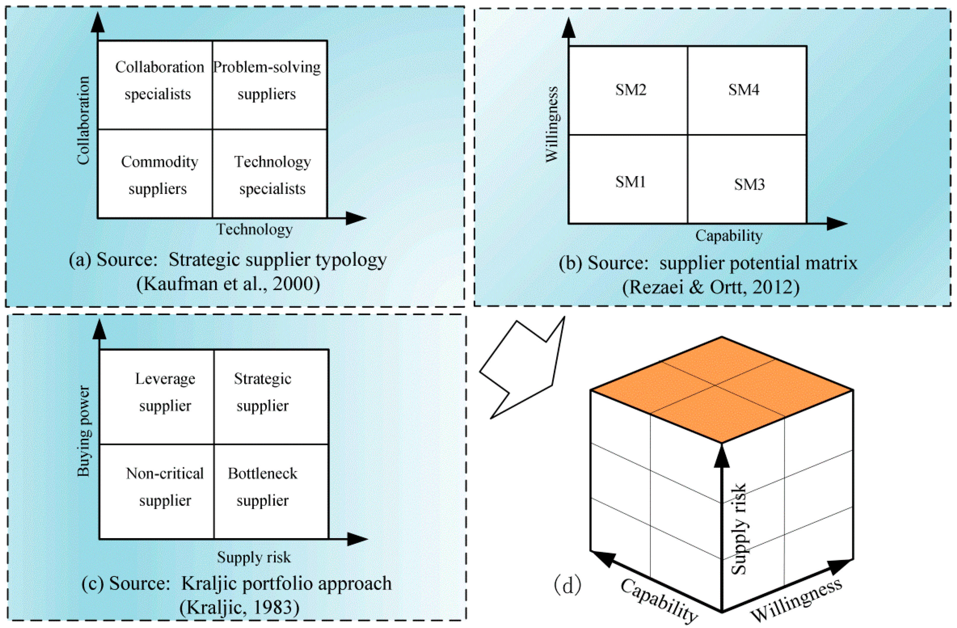
2.1. Motivation for Innovative Supplier C-W-R Evaluation

In the three dimensions of innovative supplier evaluation, there are many previous studies on the two dimensions of supplier capability and supplier willingness [34,35]. As depicted in Figure 1a, Kaufman et al. [21] segmented suppliers based on two dimensions of collaboration and technology. Then suppliers can be categorized into four groups: problem-solving suppliers, technology specialists, collaboration specialists, and commodity suppliers. Similarly, as depicted in Figure 1b, Rezaei and Ortt [34] segmented suppliers from two main dimensions of capability and willingness. However, supply risk has not yet been a major consideration in innovative supplier literature, but it should not be ignored as it is one of the most critical influences on the collaborative innovation performance especially in uncertain environments [27,48]. Since innovative components cannot be purchased directly from the display shelf, but need to be developed by both buyer and supplier [49], this requires long-term intense interaction on both sides. Thus, selecting the right innovative supplier is an important strategic decision that involves great risk [27]. For instance, as depicted in Figure 1c, Kraljic [16] considered supply risk as a variable in the purchasing portfolio model. According to this characteristic of selecting suppliers for key technical components, it is necessary to add a dimension of supply risk into the consideration of buyer–supplier collaborative innovation. Therefore, as depicted in Figure 1d, the scope of innovative supplier evaluation in this paper includes three dimensions: the supplier capability (C), the supplier willingness (W) and the supply risk (R).

2.2. Considering Supply Risk in Co-Development from a Multiproximity Perspective

The scope of supply risk varies by industry, company and even department, which is similar to prior studies investigating risk definitions, so supply risk is a multifaceted concept [27,48].

The power battery is the most critical technologically innovative component, accounting for about 30–40% of the entire production cost of NEVs [11], the cooperative development of new products between power battery suppliers and NEV manufacturers is of great significance to reduce vehicle cost. The cooperative development of new products is, however, a high-risk business, with unproven production techniques, unclear product requirements, huge up-front costs, and unreliable demand forecasts, therefore, it is necessary to premeditate the supply risk of the relationship between buyer and supplier, then the NEV manufacturer can potentially mitigate risks by working with suppliers to gain relevant expertise, knowledge, and capabilities. Therefore, supply risk is creatively considered in collaborative innovation from a multi-proximity perspective in this paper.

The French school of proximity dynamics believes that information sharing, knowledge transfer and technology acquisition between innovation subjects are affected by proximity factors, including geographical proximity, cognitive proximity, organizational proximity, social proximity, technological proximity and institutional proximity [28,50]. So supply risk in interorganizational co-developments can be defined as the geographical distance, technological distance, cognitive distance, social distance, organizational distance and institutional distance between supplier and buyer from the multi-proximity perspective. The concept of proximity refers to the types of interorganizational relationships that are expected to facilitate interactive learning and collaborative innovation [51]. Proximity may enhance absorptive capability [28] and decrease operational risk [49].

Over the past two decades, definitions of proximity have been variously framed [28,50]. Furthermore, there are some overlaps between the dimensions of different proximity concepts. For example, cognitive proximity and technological proximity are the commonalities of cognitive maps, the overlap between social proximity and relational proximity is organizational proximity [52]. In fact, physical distance is often considered a “black box” in collaborative innovation studies. As Grosjean said, “distance matters in itself, but is also a proxy for other determinants of familiarity” [52]. In this case, it is reasonable to measure supply risk in cooperative development between supplier and buyer from the multi-proximity perspective. In order to simplify the problem, this paper only consider four dimensions as the criteria to measure the amount of supply risk: geographical proximity, cognitive proximity, organizational proximity and social proximity.

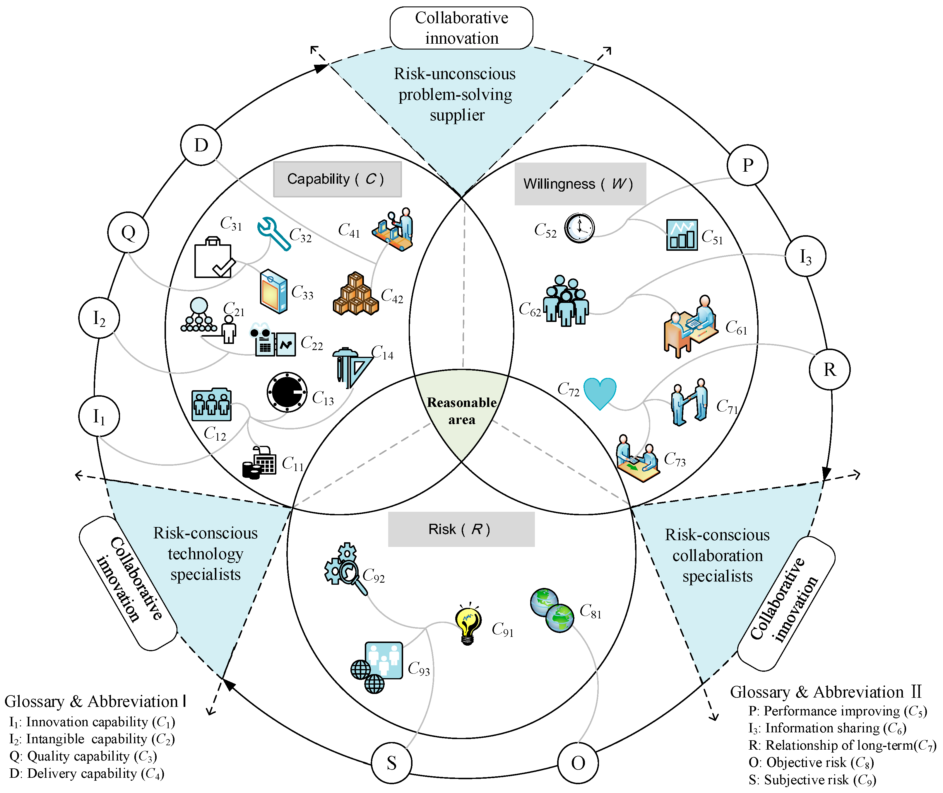
2.3. Innovative Supplier Evaluation C-W-R System

The selection of innovative suppliers should focus on whether suppliers have innovation potential, which is driven and defined by the supplier selection criteria. We now define innovative suppliers as those that have high capability and willingness to make an innovative contribution to a buying enterprise where the supply risk is as low as possible [34,35,50]. Therefore, we employ three dimensions (i.e., capability, willingness and risk) to assess the suppliers’ potential for a particular buyer.

The C-W-R evaluation is explained in the following:

• The capability of supplier (C) is defined as that a supplier could be capable of contributing innovative value for the buyers through their own complex skills and knowledge base [34,35].
• The willingness of supplier (W) is defined as a supplier that has confidence, commitment and motivation to make an innovative contribution to a buying enterprise [34,35].
• The risk of supply (R) is defined as the geographical proximity, cognitive proximity, organizational proximity and social proximity between the supplier and the buyer from a multi-proximity perspective. Proximity may decrease the cost of collaborative innovation contributing to the high probability of innovation [28,50].

As shown in Figure 2, from the NEV manufacturers’ standpoint, in order to conduct a comprehensive evaluation of the power battery innovative suppliers, only the three bubble intersection of capability (C), willingness (W) and risk (R) is considered reasonable and effective.

• If only the capability and the willingness of supplier are considered, the buying enterprise does not take supply risk into account, although a problem-solving supplier may be selected, risk-unconscious also has adverse consequences. Ignoring the proximity of the relationship between the supplier and the buyer may lead to excessive time and costs of co-development, which would impose a heavy burden on both sides of the supplier−buyer cooperative development.
• If only the capability of the supplier and the risk of supply are considered, this indicates that the supplier does not have strong willingness to be involved in cooperative development, the supplier selected belongs to a risk-conscious technology specialist. In this case, it is more likely to lead to problems in lack of trust between buyer and supplier and ineffective goal setting, which will in turn negatively affect innovation performance ensured by suppliers.
• If only the willingness of the supplier and the risk of supply are considered, the supplier would not have the capability to be involved in cooperative development, the supplier selected belongs to a risk-conscious collaboration specialist, which may result in choosing a supplier with the wrong capabilities [26], and in turn lead to lower innovation outcomes.

3. Evaluation Methodology

This section elaborates on the process of BWM-PT-VIKOR method integrating fuzzy linguistic sets.

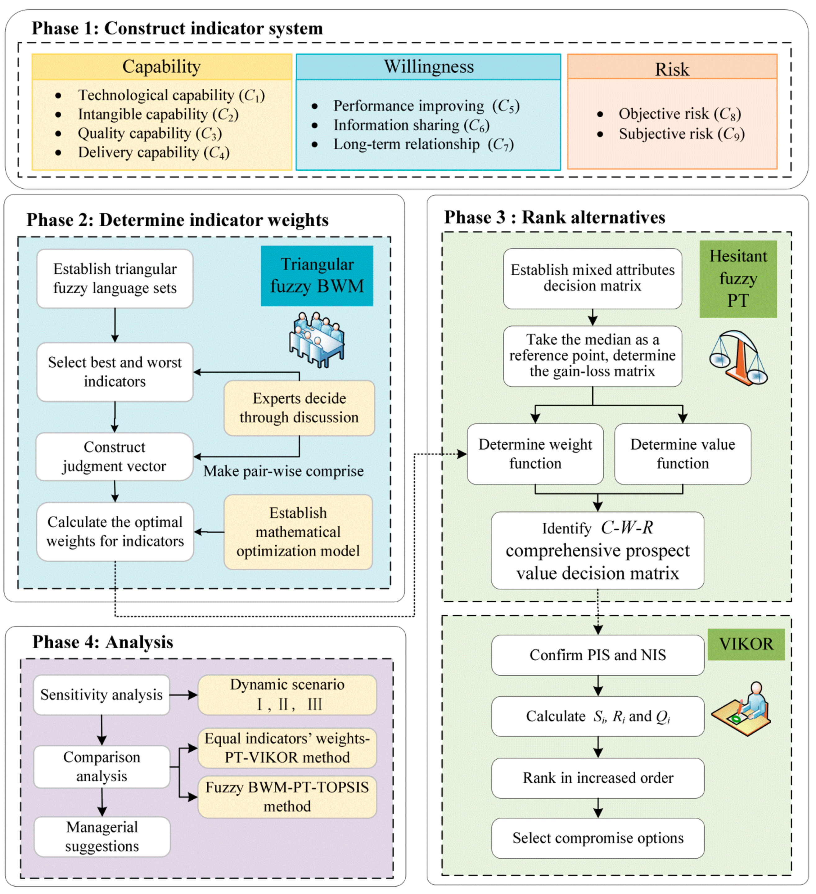
3.1. General Framework

The general framework of a hybrid BWM-PT-VIKOR method integrating fuzzy linguistic judgement is visually described in Figure 3. This method is divided into four phases: in phase 1, DMs construct the indicator system, determine alternative suppliers, and collect data by using the crisp values and hesitant fuzzy (HF) linguistic judgements; in phase 2, DMs determine weights of indicators by using fuzzy best-worst method (BWM); subsequently in phase 3, DMs need to identify a C-W-R comprehensive prospect value decision matrix, and then the VIKOR method is implemented to rank alternatives and select the compromise innovative supplier; finally in phase 4, sensitivity analysis and comparison analysis are implemented, and managerial suggestions are also presented.

3.2. C-W-R Evaluation Indicator System

On the basis of the innovative supplier definitions introduced in Section 2.1, the C-W-R evaluation indicator systems consist of 3 subsystems: the capability of supplier (denoted as C), the willingness of supplier (denoted as W) and the risk of supply (denoted as R). “C” subsystem has four factors: technical capability (denoted as C₁), intangible capability (denoted as C₂), organizational capability (denoted as C₃) and delivery capability (denoted as C₄); “W” subsystem has three factors: performance improving (denoted as C₅), information sharing (denoted as C₆) and long-term relationship (denoted as C₇); “R” subsystem has two factors: objective risk (denoted as C₈) and subjective risk (denoted as C₉). Selection of indicators is largely on the basis of previous studies about supplier selection indicators, unique characteristics of innovative supplier, and some important principles:

• Principle of consensus. Indicators need to be consistent with the logic of previous research and evaluation systems.
• Principle of representation. Indicators can represent precisely the C-W-R conditions of innovative supplier in cooperation development.
• Principle of integrity. The indicator system should not only reflect the features of innovative supplier, but also reflect the relationship of buyer−supplier collaborative innovation from the multi-proximity perspective, represented by the dimensions of supply risk.
• Principle of comparability. To make the evaluation results comparable to indicators selected by different suppliers, the concepts and calculation methods of indicators should be standardized.

Based on the above description, the C-W-R evaluation indicator system and the sources of criteria are shown in

Table 2. Criteria for innovative supplier selection.

Dimension	Criterion	Indicator	Source
Capability of supplier (C)	Technological capability (C1)	R&D expenditure input intensity (C11)	Schiele (2006) [24], Upadhyay (2012) [25]
		Relative share of R&D employees (C12)	Schiele (2006) [24], Upadhyay (2012) [25]
		Number of patents applying (C13)	Schiele (2006) [24]
		Design capability (C14)	Rezaei et al. (2015) [35]
	Intangible capability (C2)	Reputation and position in industry (C21)	Rezaei et al. (2015) [35], Choi et al. (1996) [53]
		Performance history—power battery installed capacity (C22)	Weber et al. (1991) [17], Rezaei et al. (2015) [35]
	Quality capability (C3)	Quality of product (C31)	Rezaei et al. (2015) [35], Dickson (1966) [15]
		Reliability of product (C32)	Rezaei et al. (2012) [34]
		Specific energy density of existing product (C33)	Zeng et al. (2020) [9]
	Delivery capability (C4)	Delivery satisfaction (C41)	Rezaei et al. (2015) [35], Kannan et al. (2002) [54]
		Available production capacity (C42)	Dickson (1966) [15], Weber et al. (1991) [17]
Willingness of supplier (W)	Performance improving (C5)	Commitment to continuous improvement in product and process (C51)	Rezaei et al. (2012) [34], Rezaei et al. (2015) [35], Kannan et al. (2002) [54]
		Supplier’s effort in promoting “just-in-time” principles (C52)	Rezaei et al. (2015) [35], Kannan et al. (2002) [54]
	Information sharing (C6)	Honest and frequent communications (C61)	Rezaei et al. (2015) [35], Kannan et al. (2002) [54]
		Relationship closeness (C62)	Kaufman et al. (2000) [21], Rezaei et al. (2012) [27]
	Long-term relationship (C7)	Long-term commitment (C71)	Rezaei et al. (2015) [35], Choi et al. (1996) [53]
		Mutual respect and honesty (C72)	Rezaei et al. (2012) [34], Rezaei et al. (2015) [35]
		Commitment to quality (C73)	Rezaei et al. (2015) [35], Kannan et al. (2002) [54]
Risk of supply (R)	Objective risk (C8)	Geographical proximity (C81)	Dickson (1966) [15], Schiele (2006) [24], Knoben (2006) [28], Boschma (2005) [50], Davids (2018) [51]
	Subjective risk (C9)	Cognitive proximity (C91)	Boschma (2005) [50], Davids (2018) [51]
		Organizational proximity (C92)	Boschma (2005) [50], Davids (2018) [51]
		Social proximity (C93)	Boschma (2005) [50], Davids (2018) [51]

Note: shaded areas indicate quantitative indicators.

.

3.2.1. Capability of Supplier (C) Subsystem

Capability of supplier indicates that the supplier possesses compound capability to design new products or make changes in existing products and is willing to use it in a buyer−supplier collaborative innovation [34]. There are 4 criteria and 11 indicators in this subsystem.

Technological capability (denoted as C₁) includes 4 indicators as follows:

R&D expenditure input intensity (denoted as C₁₁) is used to reflect the enterprise’s financial support for R&D activities, which is mathematically defined as:

$$C_{11}=\frac{\mathrm{R}\&\mathrm{D} \mathrm{expenditure}}{\mathrm{Sales} \mathrm{revenue}}$$

(1)

Relative share of R&D employees (denoted as C₁₂) is defined as the number of personnel engaged in research and development activities (N_R&D) divided by the total number of personnel in the corporation (N):

$$C_{12=}\frac{N_{\mathrm{R}\&\mathrm{D}}}{N}$$

(2)

Number of patents applying (denoted as C₁₃) refers to the number of achievements of scientific and technological development projects submitted by an enterprise for patent application, which is used to reflect the prevalence of independent innovation activities carried out by the enterprise.

Design capability (denoted as C₁₄) indicates the enterprise possesses the ability to control design-related issues.

Intangible capability (denoted as C₂) includes two indicators as follows: reputation and position in industry (denoted as C₂₁), which represents the company’s reputation for integrity [35] and the position of business in the market. Performance history (denoted as C₂₂) of a supplier may be captured in the supplier’s “delivery” or “quality” performance, which is the track record of business data. In this study, it is expressed by the number of power batteries installed capability which refers to the number of power batteries (single cells) actually installed into the machine (using power battery equipment), this indicator reflects the market share held by the enterprise.

Quality capability (denoted as C₃) can serve as a reflection of the ability of each supplier to meet quality specifications consistently [16], which includes three indicators as follows:

Quality (denoted as C₃₁) indicates the ability of a supplier to meet quality standards. Although reliability may be believed as a product property, buying managers identify the reliability of product (denoted as C₃₂) with the general supplier dependability [35].

Specific energy density of existing product (denoted as C₃₃) is defined as the amount of electrical energy released per unit mass of the battery, which is an important indicator of power battery performance. The endurance of NEVs mainly relies on the power battery performance, which is directly proportional to the available electricity and inversely proportional to the source energy consumption rate [9]. Under assurance of safety, with the same source energy consumption rate, battery pack volume and weight, the single maximum distance per trip of a NEV mainly depends on the energy density of the power battery.

Delivery capability (denoted as C₄) indicates the ability of a supplier to meet specified delivery schedules and quantities [17], which includes two indicators as follows:

Delivery satisfaction (denoted as C₄₁) implies that suppliers have the ability to provide fast, timely, efficient and customized services and effectively manage buyers’ complaints.

Production capacity is an important parameter to reflect the processing capacity of an enterprise, and it can also reflect the production scale of an enterprise. Available production capacity (denoted as C₄₂) implies the power of an enterprise making use of production facilities and processing in absolute numbers.

3.2.2. Willingness of Supplier (W) Subsystem

Willingness of supplier reflects a willingness to improve performance, and a willingness to maintain and develop the relationship with the buyer according to the definition of willingness proposed by Rezaei & Ortt (2012) [34]. There are three criteria and seven indicators in this subsystem.

Willingness for performance improvement (denoted as C₅) refers to the supplier’s endeavor in regard to self-improvement [35]. For suppliers, the best way to show their commitment to continuous improvement in product and process (denoted as C₅₁) is to provide better products or services. Then in the context of an uncertain environment, it is critical for supplier’s effort in promoting “just-in-time” principles (denoted as C₅₂) [54].

Willingness to information share (denoted as C₆) is an important criterion of a supplier’s willingness to maintain and develop the relationship with the buyer. Besides, a successful relationship requires trust and commitment [21,27]. It includes two indicators as follows: honest and frequent communications (C₆₁) and relationship closeness (denoted as C₆₂).

Long-term relationship (denoted as C₇) is defined as the supplier’s abiding desire to maintain a valuable relationship with the buyer [34]. For a supplier, the belief of keeping close contact with the buyer is so important that best effort should be ensured to maintain it to create a willingness for a long-term relationship with the buyer [35]. Therefore, three indicators are selected, including long-term commitment (denoted as C₇₁), mutual respect and honesty (denoted as C₇₂) and commitment to quality (denoted as C₇₃).

3.2.3. Risk of Supply (R) Subsystem

From a multi-proximity perspective, the risk of supply in interorganizational cooperative development is defined as the geographical proximity, technological proximity, cognitive proximity, social proximity, organizational proximity and institutional proximity between supplier and buyer. Because of the overlap between the different dimensions of proximity, two criteria and four indicators are selected in this subsystem.

From the view of the objective and subjective information sources, the risk of supply includes objective risk (denoted as C₈) and subjective risk (denoted as C₉). Objective risk is a distance that can be quantified, so geographical proximity (denoted as C₈₁) is defined as the distance in connection with the means of vehicle (travel time) [28]. Let T_train denote the travel time by high-speed railway from the supplier’s city to the buyer’s city, which is defined as

C₈₁ = T_train

(3)

Subjective risk (denoted as C₉) includes the following three indicators:

Cognitive proximity (denoted as C₉₁) on the enterprise level commonly refers to the similarities in the cognitive and cultural focus of the enterprise, including shared values, perspectives, knowledge base, norms of conduct and technological capabilities [29]. Since supplier and buyer are heterogeneous enterprises in the upstream and downstream of the supply chain, the higher the cognitive proximity values between them, the lower the supply risk.

Organizational proximity (denoted as C₉₂) implies sharing relationships within or between organizations, and it is conducive to collaborative innovation [28]. This dimension of proximity is in line with common principles in organizations [29]. The higher the organizational proximity values between the buyer and supplier, the lower the supply risk.

Social proximity (denoted as C₉₃) is defined as subjects that fall within the same area of relations [50]. When the buyer and the supplier are socially embedded, the probability of knowledge transfer and innovation will be greater [54]. Relations between the buyer and the supplier are socially constructed when they embrace mutual trust, common experience, and friendship [55]. The higher the social proximity values between the buyer and supplier, the lower the supply risk.

3.3. Hybrid BWM-PT-VIKOR Method Integrating Fuzzy Linguistic Sets

This section states the evaluation methodology in detail.

3.3.1. Triangular Fuzzy BWM to Determine Indicator Weight

The evaluators are experts with rich experience in the NEV field, who use triangular fuzzy linguistic terms to judge the importance of innovative supplier indicators, for triangular fuzzy linguistic terms can express human thoughts more accurately than traditional monolingual terms [42].

As shown in

Table 3. Fuzzy linguistic variable transformation rules.

Linguistic Terms	Membership Functions
Equally important (EqI)	(1,1,1)
Slightly important (SlI)	(2/3,1,3/2)
Medium important (MeI)	(3/2,2,5/2)
Very important (VeI)	(5/2,3,7/2)
Extremely important (ExI)	(7/2,4,9/2)

, these linguistic terms represent referential importance degrees. According to the principles of the BWM method, the evaluators use these triangular fuzzy linguistic terms integrating BWM method to make judgements, comparing with a best indicator to all the others, and then all the others to a worst indicator.

To convert the triangular fuzzy numbers to crisp values, the graded mean integration (denoted as GM ($\tilde{\xi }$)) is used to represent the triangular fuzzy number (denoted as $\tilde{\xi }$) [42], which is conducted as the following model:

$$GM(\tilde{\xi })=\frac{l+4\times c+u}{6}$$

(4)

where $\tilde{\xi }=\left( l , c , u \right)$, l, c, u represent the lower limit, the most likely value, and upper limit of the judged object, respectively.

For convenience, assume there are m indicators (denoted as C_j, j = 1, 2, …, m). According to the above presentation, there are four key steps of the proposed triangular fuzzy BWM.

Step 1. Determine decision criteria set {C₁, C₂, …, C_m} to evaluate alternatives. Select the best criterion C_B and the worst criterion C_W in the criteria set.

Step 2. Construct a fuzzy Best-to-Others vector:

$${\tilde{A}}_B = ({\tilde{a}}_{B1},{\tilde{a}}_{B2},{\tilde{a}}_{B3},\cdots ,{\tilde{a}}_{Bm})$$

(5)

where ${\tilde{a}}_{Bj}$ represents the fuzzy preference of the best criterion $C_B$ over criterion j,$j=1,2,\cdots , m$; ${\tilde{a}}_{Bj}=(l_{Bj},c_{Bj},u_{Bj})$ is represented by a triangular fuzzy number, it can be known that ${\tilde{a}}_{BB}=(1,1,1)$.

Step 3. Construct a fuzzy Others-to-Worst vector:

$${\tilde{A}}_{\mathrm{W}}= {({\tilde{a}}_{1W},{\tilde{a}}_{2W},{\tilde{a}}_{3W},\cdots ,{\tilde{a}}_{mW})}^T$$

(6)

where ${\tilde{a}}_{jw}$ indicates the fuzzy preference of the jth indicator over the worst indicator $C_w$; ${\tilde{a}}_{jw}=(l_{jw},c_{jw},u_{jw})$ is represented by a fuzzy number, it is clear that ${\tilde{a}}_{ww}=(1,1,1)$.

Step 4. Evaluate the optimal weights $({\tilde{\omega }}_1^{*},{\tilde{\omega }}_2^{*},\cdots ,{\tilde{\omega }}_m^{*})$.

The optimal weight for a criterion is the one where, for each pair of ${\tilde{\omega }}_B/{\tilde{\omega }}_j$ and ${\tilde{\omega }}_j/{\tilde{\omega }}_{\mathrm{w}}$, we have ${\tilde{\omega }}_B/{\tilde{\omega }}_j={\tilde{a}}_{Bj}$ and ${\tilde{\omega }}_j/{\tilde{\omega }}_w={\tilde{a}}_{jw}$. To satisfy these conditions for all j, we should find a solution where the maximum absolute differences of $\left|{\tilde{\omega }}_B/{\tilde{\omega }}_j-{\tilde{a}}_{Bj}\right|$ and $\left|{\tilde{\omega }}_j/{\tilde{\omega }}_w-{\tilde{a}}_{jw}\right|$ for all j are minimized. Let ${\tilde{\omega }}_B=(l_B^{\omega },c_B^{\omega },u_B^{\omega })$, ${\tilde{\omega }}_j=(l_j^{\omega },c_j^{\omega },u_j^{\omega })$, ${\tilde{\omega }}_{\mathrm{w}}=(l_w^{\omega },c_w^{\omega },u_w^{\omega })$, $\tilde{\xi }=(l_{}^{\omega },c_{}^{\omega },u_{}^{\omega })$, ${\tilde{\xi }}^{*}=(t^{*},t^{*},t^{*})$, $t^{*}\le l^{\omega }$, considering the non-negativity and sum condition for the weights, the constrained optimization problem could be attained as follows:

$$\begin{array}{l}\min {\xi }^{*}\\ s.t.\{\begin{array}{c}\left|\frac{(l_B^{\omega },c_B^{\omega },u_B^{\omega })}{(l_j^{\omega },c_j^{\omega },u_j^{\omega })}-(l_{Bj}^{},c_{Bj}^{},u_{Bj}^{})\right|\le \{t^{*},t^{*},t^{*}\}\hfill \\ \left|\frac{(l_j^{\omega },c_j^{\omega },u_j^{\omega })}{(l_W^{\omega },c_W^{\omega },u_W^{\omega })}-(l_{jW}^{},c_{jW}^{},u_{jW}^{})\right|\le \{t^{*},t^{*},t^{*}\}\hfill \\ {\displaystyle \sum _{j=1}^{n}GM({\tilde{\omega }}_j)=1}\hfill \\ \begin{array}{l}{l}_j^{\omega }\le c_j^{\omega }\le u_j^{\omega }\hfill \\ l_j^{\omega }\ge 0\hfill \\ j=1,\cdots ,m\hfill \end{array}\hfill \end{array}\end{array}$$

(7)

Solution of the above equations provides the optimal fuzzy weight of indicator $({\tilde{\omega }}_1^{*},{\tilde{\omega }}_2^{*},\cdots ,{\tilde{\omega }}_{\mathrm{m}}^{*})$.

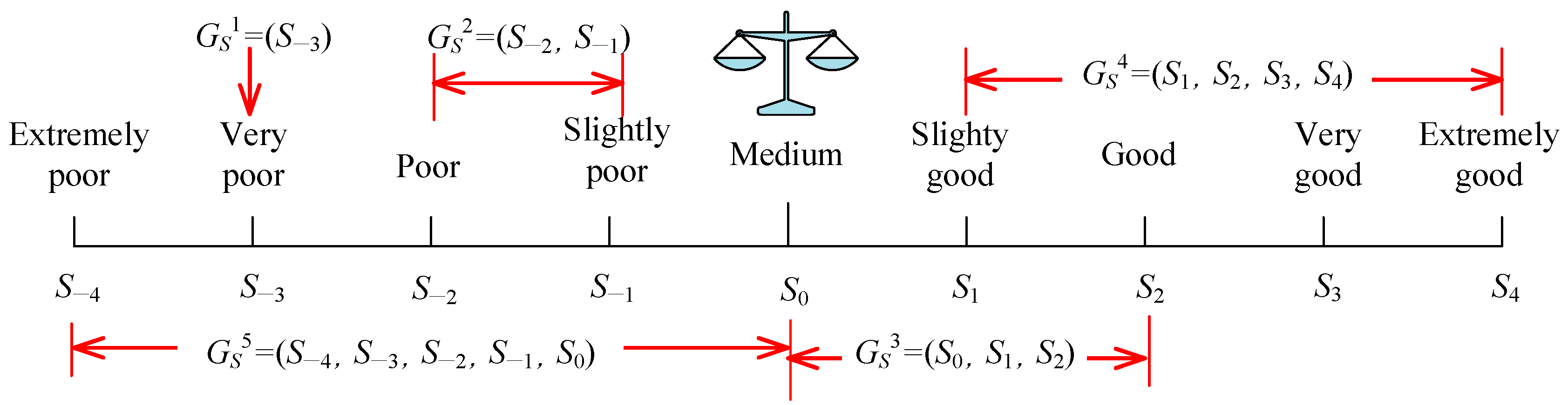
3.3.2. Extended PT-VIKOR Integrating Hesitant Fuzzy Linguistic Sets for Ranking Alternatives

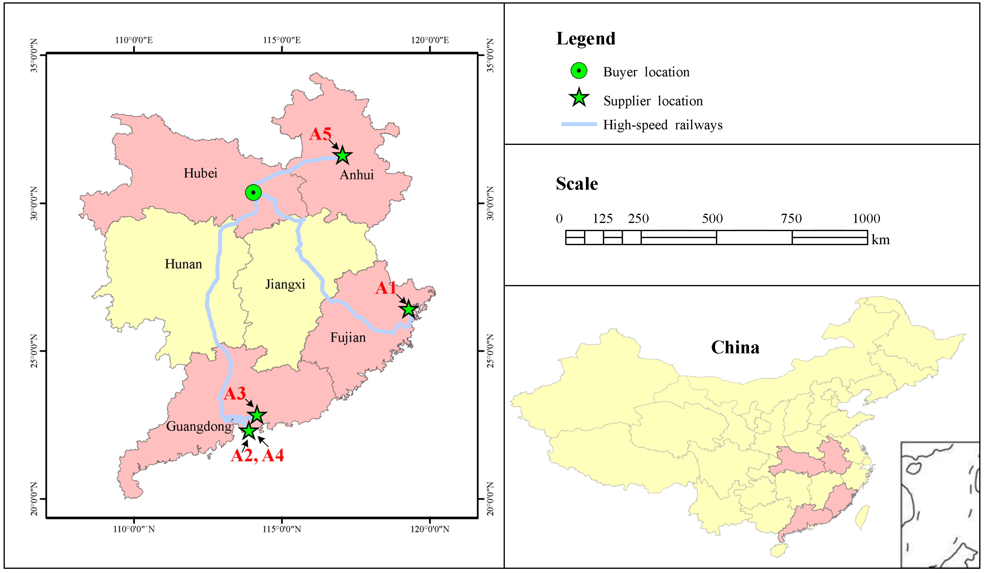
To conform to the reality of the MCDM problem, hesitant fuzzy linguistic sets are employed to represent the expert assessment values of the C-W-R qualitative indicators, since this judgement method is of flexibility and capability of avoiding information loss to the best extent possible [43].

Let S = {$S_{\alpha }$|α = −τ, …, −1, 0, 1, …, τ} be a symmetrical linguistic term set [42,43], when 9-scale is adopted symmetrically: $S = \left\{S_{-4},S_{-3},S_{-2},S_{-1},S_0,S_1,S_2,S_3,S_4\right\}$ = {extremely poor, very poor, poor, slightly poor, medium, slightly good, good, very good, extremely good}, the linguistic variable G_S^x can be interpreted as a fuzzy restriction label.

For example, for indicator “mutual respect and honesty”, the linguistic information attained by using hesitant fuzzy linguistic judgements might be: φ₁ = extremely poor, φ₂ = between poor and slightly poor, φ₃ = between medium and good, probably slightly good, φ₄ = greater than slightly good, φ₅ = not exceed medium. As shown in Figure 4, the above linguistic information can be denoted as G_S¹ = (S₋₃), G_S² = (S₋₂, S₋₁), G_S³ = (S₀, S₁, S₂), G_S⁴ = (S₁, S₂, S₃, S₄), G_S⁵ = (S₋₄, S₋₃, S₋₂, S₋₁, S₀).

To ensure comparability, it is requisite to extend the shorter G_S^x to the same length [45]. The extension rule is $\overline{h} = \eta h^{+} +\left( 1 - \eta \right) h{ }^{–}$, where η (0 ≤ η ≤ 1) is the parameter determined based on the experts’ attitudes [45], and h⁺ and h⁻ are respectively the maximal and the minimal values in G_S^x. In this paper, η = 0.5, which means experts take neutral attitudes [46]. Extended examples can be seen in

Table 4. Extended examples of hesitant fuzzy judgements.

Original Judgements	Extensions
GS1 = (S−3)	(S−3, S−3, S−3, S−3, S−3)
GS2 = (S−2, S−1)	(S−2, S−1.5, S−1.5, S−1.5, S−1)
GS3 = (S0, S1, S2)	(S0, S1, S1, S1, S2)
GS4 = (S1, S2, S3, S4)	(S1, S2, S2.5, S3, S4)
GS5 = (S−4, S−3, S−2, S−1, S0)	(S−4, S−3, S−2, S−1, S0)

.

There are seven steps of the extended PT-VIKOR integrating hesitant fuzzy linguistic sets method for ranking alternatives.

Step 1. Construct the mixed attribute matrix N and normalize matrix.

A1 … Ap … Am

$$N=\begin{array}{c}{C}_{11}\\ C_{12}\\ ⋮\\ C_{nm}\end{array}\left[\begin{array}{c}{g}_{11}\\ g_{21}\\ ⋮\\ G_S{}_{n1}\end{array}\begin{array}{c}\cdots \\ \cdots \\ \cdots \\ \cdots \end{array}\begin{array}{c}{g}_{1p}\\ g_{2p}\\ ⋮\\ G_S{}_{np}\end{array}\begin{array}{c}\cdots \\ \cdots \\ \ddots \\ \cdots \end{array}\begin{array}{c}{g}_{1m}\\ g_{2m}\\ ⋮\\ G_S{}_{nm}\end{array}\right]$$

(8)

In the above decision matrix, $g_{ij}$ represents the crisp indicator and $G_S{}_{ij}$ denotes the hesitant fuzzy indicator. Let $J_C$ and $J_H$ respectively denote the crisp indicator set and the hesitant fuzzy indicator set. For benefit-indicator, it gives

$${\mathrm{g}}_{ij}^{\prime }=\left\{\frac{g_i{}_j-\min \left\{g_i{}_j\right\}}{\max \left\{g_i{}_j\right\}-\min \left\{g_i{}_j\right\}}|i=1,2,\cdots ,m,j\in J_C\right\}$$

(9)

For cost-indicator, it gives

$${\mathrm{g}}_{ij}^{\prime }=\left\{\frac{\max \left\{g_i{}_j\right\}-g_i{}_j}{\max \left\{g_i{}_j\right\}-\min \left\{g_i{}_j\right\}}|i=1,2,\cdots ,m,j\in J_C\right\}$$

(10)

Step 2. Take the median as the reference point and determine the Gain-loss matrix.

For measuring the closeness degrees and deviation of two different but equal-length hesitant fuzzy sets, distance and similarity measures are commonly used tools widely [47]. In this paper, Hamming distance is employed to measure hesitant fuzzy set $G_S{}_{ij}$ to the median hesitant fuzzy set $G_S^{\mathrm{medium}}$.

$$d\left(G_S{}_{ij},G_S^{\mathrm{medium}}\right)=\frac{1}{L}{\displaystyle \sum _{l=1}^L\frac{\left|{\delta }_l^1-{\delta }_l^2\right|}{2\tau +1}},i=1,2,\cdots ,m,j=p,p+1,\cdots ,n,j\in J_H$$

(11)

where $G_S{}_{ij}={\cup }_S{{}_{{\delta }_l^1}}_{\in G_S{}_{ij}}\{s_{{\delta }_l^1}|l=1,\cdots ,L\}$, $G_S^{\mathrm{medium}}={\cup }_S{{}_{{\delta }_l^2}}_{\in G_S^{\mathrm{medium}}}\{s_{{\delta }_l^2}|l=1,\cdots ,L\}$, L is the number of linguistic terms and 1 ≤ L ≤ 9 in this paper.

For the indicators that have crisp values, ${\mathrm{g}}_{{}_j}^{\mathrm{medium}}$ donates the median value, the generation of $d\left({\mathrm{g}}_{ij},{\mathrm{g}}_{{}_j}^{\mathrm{medium}}\right)$ are given below:

$$d\left({\mathrm{g}}_{ij},{\mathrm{g}}_{{}_j}^{\mathrm{medium}}\right)=\left|{\mathrm{g}}_{ij}-{\mathrm{g}}_{{}_j}^{\mathrm{medium}}\right|,i=1,2,\cdots ,m,j=1,2,\cdots ,p-1,j\in J_C$$

(12)

Step 3. Determine the weight function and the value function, and then calculate the prospect value of each indicator.

Considering comparison rules of the two hesitant fuzzy linguistic term sets [41], the value functions of linguistic indicators are determined in the following:

$$v(x_{ij})=\{\begin{array}{cc}-\lambda {(d(G_S{}_{ij},G_S^{\mathrm{medium}}))}^{\beta }\hfill & {\mathrm{g}}_{ij}<{\mathrm{g}}_{{}_j}^{\mathrm{medium}} \mathrm{or} G_S{}_{ij}\prec G_S^{\mathrm{medium}}\hfill \\ 0\hfill & {\mathrm{g}}_{ij}={\mathrm{g}}_{{}_j}^{\mathrm{medium}} \mathrm{or} G_S{}_{ij}\cong G_S^{\mathrm{medium}}\hfill \\ {(d(G_S{}_{ij},G_S^{\mathrm{medium}}))}^{\alpha }\hfill & {\mathrm{g}}_{ij}>{\mathrm{g}}_{{}_j}^{\mathrm{medium}} \mathrm{or} G_S{}_{ij}\succ G_S^{\mathrm{medium}}\hfill \end{array}$$

(13)

where α and β are adjustable coefficients satisfying the constraints 0 ≤ α, β ≤ 1, λ depicts loss aversion satisfying generally λ > 1, and α = β = 0.88, λ = 2.25 in this paper [41].

On the basis of the definition of PT, indicators’ weights are determined by using the following equation:

$$w(p_{ij})=\{\begin{array}{c}\frac{p_{Ij}^{\delta }}{{\left[p_{Ij}^{\delta }+{(1-p_{Ij}^{})}^{\delta }\right]}^{\raisebox{1ex}{$1$}\!\left/ \!\raisebox{-1ex}{$\delta $}\right.}}{ \mathrm{g}}_{ij}{<\mathrm{g}}_{{}_j}^{\mathrm{medium}} \mathrm{or} G_S{}_{ij}\prec G_S^{\mathrm{medium}}\\ \frac{p_{Ij}^{\gamma }}{{\left[p_{Ij}^{\gamma }+{(1-p_{Ij}^{})}^{\gamma }\right]}^{\raisebox{1ex}{$1$}\!\left/ \!\raisebox{-1ex}{$\gamma $}\right.}}{ \mathrm{g}}_{ij}>{\mathrm{g}}_{{}_j}^{\mathrm{medium}} \mathrm{or} G_S{}_{ij}\succ G_S^{\mathrm{medium}}\end{array}$$

(14)

where γ and δ represent the risk attitude coefficients with gains and losses expectations, respectively, generally, γ takes 0.61 and δ takes 0.69 [38].

Determine the prospect values of the indicators as follows:

$$V(x_{ij})=v(x_{ij})·w(p_{ij})$$

(15)

Step 4. Calculate the composite prospect value of C-W-R, construct the C-W-R prospect decision matrix, and determine the positive ideal solution (PIS) and the negative ideal solution (NIS) respectively by Equations (16) and (17):

$$V_i^{*}=\{\max V_{i1},\max V_{i2},\cdots ,\max V_{i\mathrm{n}}\}$$

(16)

$$V_i^{-}=\{\min V_{i1},\min V_{i2},\cdots ,\min V_{i\mathrm{n}}\}$$

(17)

Step 5. Calculate the values of group utility S_j and individual regret R_j by Equations (18) and (19):

$$S_i={\displaystyle \sum _{i=1}\frac{{\omega }_j^c(V_i^{*}-V_{ij})}{(V_i^{*}-V^{-})}}$$

(18)

$$R_i=\underset{i}{\max }\frac{{\omega }_j^c(V_i^{*}-V_{ij})}{(V_i^{*}-V^{-})}$$

(19)

where ${\omega }_j^c$ is the weight of indicator j.

Step 6. Calculate the value of Q_i (i = 1, 2, …, n) by Equation (20):

$$Q_i=\frac{v(S_i-S^{-})}{S^{*}-S^{-}}+\frac{(1-v)(R_i-R^{-})}{R^{*}-R^{-}}$$

(20)

where S^∗ = max S_i, S⁻ = min S_i, R^∗ = max R_i, R⁻ = min R_i and ν is introduced as weight of the strategy of “the majority of criteria”, without loss of generality, ν takes 0.5 in this paper.

Step 7. Rank the alternatives, sorting by the values S_i, R_i and Q_i in ascending order, and determine the compromise solution.

A compromise solution (alternatives Aa, a =1, 2, …, r) which has the smallest value of Q_a (a = 1, 2, …, r) (i.e., ranking first in the list) can be determined if the following two conditions are satisfied [41]:

Condition 1. “Acceptable advantage”:

$$Q_{a^{\prime }}-Q_a\ge \frac{1}{r-1}$$

(21)

where Q_a’ (a’ = 1, 2, …, r) is in the second position for Q_i (i = 1, 2, …, r) in the ranking list.

Condition 2. “Acceptable stability in decision making”: If alternative Aa ranks first based on Q_a, then it should also have the best performance based on S_a and R_a.

If condition 1 is not satisfied, we can get the compromise solutions through $Q_{a\prime }-Q_a<1/(r-1)$, where i, a = 1, 2, …, r, I ≠ a; if condition 2 is not satisfied, the alternatives that rank first and second are both the compromise solutions.

4. Case Study

In this section, the power battery supplier selection for NEVs is taken for case study, and the results are presented in the following.

4.1. Case Description

The development of NEVs is a strategic intersection of national energy security, energy conservation and emission reduction, environmental governance and even the development of emerging industries and the upgrading of traditional industries [1]. Especially led by innovation-driven strategy, many automobile manufacturers and supporting enterprises are committed to launching their own NEV competitive products. However, the power battery, as the most critical technologically innovative component of NEVs, is the feeble section and the main obstacle of the industrialization of NEVs.

To improve the performance of the power battery, H Company prepared to install a Battery Cooperative Research and Development Center in Hubei province (see Figure 5). H Company, a leader in the mainland’s NEV industry, is at the core of the supply chain with a well-organized network of suppliers and is now listed in Hong Kong. On the basis of the specifications for automotive power storage batteries, according to the preliminary examination results of the bidding enterprises, five alternative suppliers namely A1, A2, A3, A4 and A5 were picked out. To better select the optimal innovative supplier(s) to establish a strategic partnership for collaborative innovation, a review conference was held in Wuhan, Hubei province. Based on the evaluation, this paper proposes some managerial suggestions to help H Company to select the problem-solving innovative supplier(s) for obtaining buyer–supplier collaborative innovation performance under the conditions of considering the supply risk.

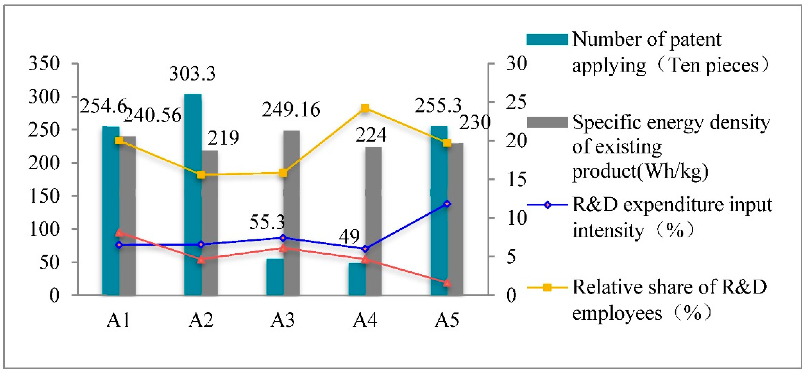
4.2. Data Collection and Processing

Considering the different data types, 22 indicators fall into two categories in this evaluation system. The first category includes R&D expenditure input intensity (C₁₁), relative share of R&D employees (C₁₂), number of patents applying (C₁₃), performance history—power battery installed base (C₂₂), specific energy density of existing product (C₃₃), available production capacity (C₄₂) and geographical proximity (C₈₁), because their accurate values can be attained using the technical schemes, annual reports of listed companies and the bidding documents.

The second category is the one with qualitative indicators, which are difficult to directly obtain accurate values. To better handle hesitancy and fuzziness in the process of expert evaluation, a more efficient and applicable way may be to employ linguistic judgements rather than exact numeric values. This study uses hesitant fuzzy linguistic judgements to reduce information loss and state the judgement results [46]. Experts pick the appropriate linguistic values (extremely poor, very poor, poor, slightly poor, medium, slightly good, good, very good, and extremely good) according to product introductions, the financial statements, bidding documents, industry reports and relevant case information, the original data of the five alternative suppliers is shown in

Table A1. Original data of the five alternative suppliers.

	A1	A2	A3	A4	A5
C11 (%)	6.53	6.59	7.44	6.03	11.86
C12 (%)	20.03	15.62	15.85	24.23	19.73
C13 (Piece)	2546	3033	553	490	2553
C14	between good and very good	greater than good	between slightly good and good	between medium and good	between slightly good and very good
C21	greater than good	greater than good	between medium and slightly good	between medium and slightly good	between medium and good
C22 (Gwh/year)	32.31	10.78	1.84	0.65	3.22
C31	between good and very good	between good and very good	medium	between medium and slightly good	between slightly good and very good
C32	greater than good	between good and very good	medium	medium	between slightly good and good
C33 (Wh/kg)	240.56	219	249.16	224	230
C41	between good and very good	greater than good	between medium and good	between medium and slightly good	between slightly good and good
C42 (Gwh/year)	35	30	12	4	14
C51	greater than very good	greater than good	between slightly good and good	between slightly good and good	between good and very good
C52	greater than good	greater than very good	between slightly good and good	between slightly good and good	greater than very good
C61	greater than good	greater than good	between good and very good	between good and very good	greater than good
C62	greater than good	greater than good	between good and very good	between good and very good	greater than good
C71	greater than good	between good and very good	between slightly good and very good	between slightly good and very good	greater than good
C72	greater than very good	greater than good	between good and very good	between good and very good	greater than good
C73	greater than good	between good and very good	between slightly good and very good	between slightly good and very good	greater than good
C81 (Hours)	8.15	4.67	6.14	4.67	1.64
C91	greater than good	between slightly good and very good	between medium and slightly good	between medium and slightly good	greater than good
C92	between slightly good and very good	greater than good	between medium and slightly good	between medium and slightly good	between medium and good
C93	between good and very good	greater than good	between medium and slightly good	between slightly poor and slightly good	between medium and good

of Appendix A, the normalized decision matrix is shown in

Table 5. Normalized decision matrix.

	A1	A2	A3	A4	A5
C11	0.086	0.096	0.242	0.000	1.000
C12	0.512	0.000	0.027	1.000	0.477
C13	0.809	1.000	0.025	0.000	0.811
C14	(S2, S2.5, S3)	(S2, S3, S4)	(S1, S1.5, S2)	(S0, S1, S2)	(S1, S2, S3)
C21	(S2, S3, S4)	(S2, S3, S4)	(S0, S0.5, S1)	(S0, S0.5, S1)	(S0, S1, S2)
C22	1.000	0.320	0.038	0.000	0.081
C31	(S2, S2.5, S3)	(S2, S2.5, S3)	(S0, S0, S0)	(S0, S0.5, S1)	(S1, S2, S3)
C32	(S2, S3, S4)	(S2, S2.5, S3)	(S0, S0, S0)	(S0, S0, S0)	(S1, S1.5, S2)
C33	0.715	0.000	1.000	0.166	0.365
C41	(S2, S2.5, S3)	(S2, S3, S4)	(S0, S1, S2)	(S0, S0.5, S1)	(S1, S1.5, S2)
C42	1.000	0.839	0.258	0.000	0.323
C51	(S3, S3.5, S4)	(S2, S3, S4)	(S1, S1.5, S2)	(S1, S1.5, S2)	(S2, S2.5, S3)
C52	(S2, S3, S4)	(S3, S3.5, S4)	(S1, S1.5, S2)	(S1, S1.5, S2)	(S3, S3.5, S4)
C61	(S3, S3.5, S4)	(S2, S3, S4)	(S2, S2.5, S3)	(S2, S2.5, S3)	(S3, S3.5, S4)
C62	(S3, S3.5, S4)	(S2, S3, S4)	(S2, S2.5, S3)	(S2, S2.5, S3)	(S3, S3.5, S4)
C71	(S2, S3, S4)	(S2, S2.5, S3)	(S1, S2, S3)	(S1, S2, S3)	(S2, S3, S4)
C72	(S3, S3.5, S4)	(S2, S3, S4)	(S2, S2.5, S3)	(S2, S2.5, S3)	(S3, S3.5, S4)
C73	(S2, S3, S4)	(S2, S2.5, S3)	(S1, S2, S3)	(S1, S2, S3)	(S2, S3, S4)
C81	0.000	0.535	0.309	0.535	1.000
C91	(S2, S3, S4)	(S1, S2, S3)	(S0, S0.5, S1)	(S0, S0.5, S1)	(S3, S3.5, S4)
C92	(S1, S2, S3)	(S2, S3, S4)	(S0, S0.5, S1)	(S0, S0.5, S1)	(S0, S1, S2)
C93	(S2, S2.5, S3)	(S2, S3, S4)	(S0, S0.5, S1)	(S-1, S0, S1)	(S0, S1, S2)

, and detailed data processing are shown in

Table A2. Normalized decision matrix for J_C.

	A1	A2	A3	A4	A5
C11	0.0858	0.0961	0.2419	0.0000	1.0000
C12	0.5122	0.0000	0.0267	1.0000	0.4774
C13	0.8085	1.0000	0.0248	0.0000	0.8112
C22	1.0000	0.3200	0.0376	0.0000	0.0812
C33	0.7149	0.0000	1.0000	0.1658	0.3647
C42	1.0000	0.8387	0.2581	0.0000	0.3226
C81	0.0000	0.5346	0.3088	0.5346	1.0000

,

Table A3. Conversion of hesitant fuzzy linguistic judgement decision matrix for J_H.

	A1	A2	A3	A4	A5
C14	(S2, S3)	(S2, S3, S4)	(S1, S2)	(S0, S1, S2)	(S1, S2, S3)
C21	(S2, S3, S4)	(S2, S3, S4)	(S0, S1)	(S0, S1)	(S0, S1, S2)
C31	(S2, S3)	(S2, S3)	(S0)	(S0, S1)	(S1, S2, S3)
C32	(S2, S3, S4)	(S2, S3)	(S0)	(S0)	(S1, S2)
C41	(S2, S3)	(S2, S4)	(S0, S1, S2)	(S0, S1)	(S1, S2)
C51	(S3, S4)	(S2, S4)	(S1, S2)	(S1, S2)	(S2, S3)
C52	(S2, S3, S4)	(S3, S4)	(S1, S2)	(S1, S2)	(S3, S4)
C61	(S3, S4)	(S2, S3, S4)	(S2, S3)	(S2, S3)	(S3, S4)
C62	(S3, S4)	(S2, S3, S4)	(S2, S3)	(S2, S3)	(S3, S4)
C71	(S2, S3, S4)	(S2, S3)	(S1, S2, S3)	(S1, S2, S3)	(S2, S3, S4)
C72	(S3, S4)	(S2, S3, S4)	(S2, S3)	(S2, S3)	(S3, S4)
C73	(S2, S3, S4)	(S2, S3)	(S1, S2, S3)	(S1, S2, S3)	(S2, S3, S4)
C91	(S2, S3, S4)	(S1, S2, S 3)	(S0, S1)	(S0, S1)	(S3, S4)
C92	(S1, S2, S3)	(S2, S3, S4)	(S0, S1)	(S0, S1)	(S0, S1, S2)
C93	(S2, S3)	(S2, S3, S4)	(S0, S1)	(S−1, S0, S1)	(S0, S1, S2)

and

Table A4. Extended hesitant fuzzy numbers decision matrix for J_H.

	A1	A2	A3	A4	A5
C14	(S2, S2.5, S3)	(S2, S3, S4)	(S1, S1.5, S2)	(S0, S1, S2)	(S1, S2, S3)
C21	(S2, S3, S4)	(S2, S3, S4)	(S0, S0.5, S1)	(S0, S0.5, S1)	(S0, S1, S2)
C31	(S2, S2.5, S3)	(S2, S2.5, S3)	(S0, S0, S0)	(S0, S0.5, S1)	(S1, S2, S3)
C32	(S2, S3, S4)	(S2, S2.5, S3)	(S0, S0, S0)	(S0, S0, S0)	(S1, S1.5, S2)
C41	(S2, S2.5, S3)	(S2, S3, S4)	(S0, S1, S2)	(S0, S0.5, S1)	(S1, S1.5, S2)
C51	(S3, S3.5, S4)	(S2, S3, S4)	(S1, S1.5, S2)	(S1, S1.5, S2)	(S2, S2.5, S3)
C52	(S2, S3, S4)	(S3, S3.5, S4)	(S1, S1.5, S2)	(S1, S1.5, S2)	(S3, S3.5, S4)
C61	(S3, S3.5, S4)	(S2, S3, S4)	(S2, S2.5, S3)	(S2, S2.5, S3)	(S3, S3.5, S4)
C62	(S3, S3.5, S4)	(S2, S3, S4)	(S2, S2.5, S3)	(S2, S2.5, S3)	(S3, S3.5, S4)
C71	(S2, S3, S4)	(S2, S2.5, S3)	(S1, S2, S3)	(S1, S2, S3)	(S2, S3, S4)
C72	(S3, S3.5, S4)	(S2, S3, S4)	(S2, S2.5, S3)	(S2, S2.5, S3)	(S3, S3.5, S4)
C73	(S2, S3, S4)	(S2, S2.5, S3)	(S1, S2, S3)	(S1, S2, S3)	(S2, S3, S4)
C91	(S2, S3, S4)	(S1, S2, S3)	(S0, S0.5, S1)	(S0, S0.5, S1)	(S3, S3.5, S4)
C92	(S1, S2, S3)	(S2, S3, S4)	(S0, S0.5, S1)	(S0, S0.5, S1)	(S0, S1, S2)
C93	(S2, S2.5, S3)	(S2, S3, S4)	(S0, S0.5, S1)	(S-1, S0, S1)	(S0, S1, S2)

of Appendix A.

4.3. Results Interpretation

This section interprets the results of the calculation using C-W-R evaluation methodology.

4.3.1. Fuzzy BWM Results for Weight of Each Indicator

Through the analysis of all 22 indicators, experts reach an agreement through discussion that C₁₁ is the best indicator and C₉₃ is the worst indicator. Compare the best indicator with all other indicators, and similarly other indicators with the worst indicator using the corresponding triangular fuzzy language judgments. Based on this, the final crisp weights are determined using model (7) and Equation (4) with Lingo11, which is shown as follows, and the detailed data processing are shown in

Table A5. Triangular fuzzy rating of the best indicator compared with each indicator.

Indicator	C11	C12	C13	C14	C21
Best indicator C11	EqI (1, 1, 1)	EqI (1, 1, 1)	SlI (2/3, 1, 3/2)	SlI (2/3, 1, 3/2)	SlI (2/3, 1, 3/2)
Indicator	C22	C31	C32	C33	C41
Best indicator C11	MeI (3/2, 2, 5/2)	SlI (2/3, 1, 3/2)	SlI (2/3, 1, 3/2)	EqI (1, 1, 1)	VeI (5/2, 3, 7/2)
Indicator	C42	C51	C52	C61	C62
Best indicator C11	VeI (5/2, 3, 7/2)	VeI (5/2, 3, 7/2)	VeI (5/2, 3, 7/2)	EqI (1, 1, 1)	EqI (1, 1, 1)
Indicator	C71	C72	C73	C81	C91
Best indicator C11	SlI (2/3, 1, 3/2)	EqI (1, 1, 1)	SlI (2/3, 1, 3/2)	ExI (7/2, 4, 9/2)	VeI (5/2, 3, 7/2)
Indicator	C92	C93
Best indicator C11	ExI (7/2, 4, 9/2)	ExI (7/2, 4, 9/2)

and

Table A6. Triangular Fuzzy ratings of all indicators compared with the worst indicator.

Indicator	Worst Indicator C93	Indicator	Worst Indicator C93	Indicator	Worst Indicator C93
C11	ExI (7/2, 4, 9/2)	C33	ExI (7/2, 4, 9/2)	C72	ExI (7/2, 4, 9/2)
C12	ExI (7/2, 4, 9/2)	C41	VeI (5/2, 3, 7/2)	C73	VeI (5/2, 3, 7/2)
C13	VeI (5/2, 3, 7/2)	C42	VeI (5/2, 3, 7/2)	C81	VeI (5/2, 3, 7/2)
C14	VeI (5/2, 3, 7/2)	C51	VeI (5/2, 3, 7/2)	C91	VeI (5/2, 3, 7/2)
C21	VeI (5/2, 3, 7/2)	C52	MeI (3/2, 2, 5/2)	C92	EqI (1, 1, 1)
C22	MeI (3/2, 2, 5/2)	C61	ExI (7/2, 4, 9/2)	C93	EqI (1, 1, 1)
C31	VeI (5/2, 3, 7/2)	C62	ExI (7/2, 4, 9/2)
C32	VeI (5/2, 3, 7/2)	C71	VeI (5/2, 3, 7/2)

of Appendix A.

$w\left(p_{ij}\right)$ = {0.080, 0.056, 0.047, 0.052, 0.052, 0.029, 0.052, 0.054, 0.061, 0.037, 0.032, 0.032, 0.040, 0.061, 0.056, 0.052, 0.053, 0.052, 0.029, 0.032, 0.026, 0.016}.

4.3.2. Consistency Ratio Checking

To ensure pairwise comparisons’ validity, consistency ratio (CR) should be considered. According to consistency index (CI) for fuzzy BWM [42], ${\tilde{a}}_{BW}$ is selected as (7/2, 4, 9/2) in this paper, for this case, the CI value is 8.04, and that ${\xi }^{\ast }=1.172,$ so the CR is $\raisebox{1ex}{$1.172$}\!\left/ \!\raisebox{-1ex}{$8.04$}\right. = 0.146$, which means a high level of consistency in this case since the CR value 0.146 is far less than 1 and close to zero.

4.3.3. C-W-R Evaluation Results with PT-VIKOR

After obtaining the indicators’ weights, the subsequent evaluation calculation will be carried out with PT-VIKOR method.

(1)

Determine the C-W-R comprehensive prospect value decision matrix.

Based on Equations (11) and (12), we obtain the gain-loss matrix as shown in

Table 6. Gain-loss matrix.

	A1	A2	A3	A4	A5
C11	−0.010	0.000	0.146	−0.096	0.904
C12	0.035	−0.477	−0.451	0.523	0.000
C13	0.000	0.192	−0.784	−0.809	0.003
C14	0.056	0.111	−0.056	−0.111	0.000
C21	0.222	0.222	−0.056	−0.056	0.000
C22	0.919	0.239	−0.044	−0.081	0.000
C31	0.056	0.056	−0.222	−0.167	0.000
C32	0.167	0.111	−0.167	−0.167	0.000
C33	0.350	−0.365	0.635	−0.199	0.000
C41	0.111	0.167	−0.056	−0.111	0.000
C42	0.677	0.516	−0.065	−0.323	0.000
C51	0.111	0.056	−0.111	−0.111	0.000
C52	0.000	0.056	−0.167	−0.167	0.056
C61	0.056	0.000	−0.056	−0.056	0.056
C62	0.056	0.000	−0.056	−0.056	0.056
C71	0.056	0.000	−0.056	−0.056	0.056
C72	0.056	0.000	−0.056	−0.056	0.056
C73	0.056	0.000	−0.056	−0.056	0.056
C81	−0.535	0.000	−0.226	0.000	0.465
C91	0.111	0.000	−0.167	−0.167	0.167
C92	0.111	0.222	−0.056	−0.056	0.000
C93	0.167	0.222	−0.056	−0.111	0.000

.

According to the weight function definition of PT, when DMs are in the profit situation, based on Equation (14), we have

$w^{+}\left(p_{ij}\right)$ = {0.167, 0.140, 0.127, 0.134, 0.134, 0.099, 0.134, 0.137, 0.146, 0.113, 0.105, 0.105, 0.117, 0.146, 0.140, 0.134, 0.136, 0.134, 0.098, 0.105, 0.093, 0.071}.

When DMs are in the loss situation, based on Equation (14), we obtain

$w^{-}\left(p_{ij}\right)$ = {0.149, 0.120, 0.107, 0.114, 0.114, 0.079, 0.114, 0.117, 0.126, 0.093, 0.085, 0.085, 0.097, 0.126, 0.120, 0.114, 0.116, 0.114, 0.078, 0.084, 0.074, 0.053}.

According to Equation (15), the prospect value matrix and the C-W-R comprehensive prospect value decision matrix could be obtained as depicted in

Table 7. The C-W-R comprehensive prospect value decision matrix.

	A1	A2	A3	A4	A5
C	0.422	0.062	−0.208	−0.311	0.263
W	0.152	0.107	0.000	0.000	0.146
R	−0.026	0.079	−0.042	0.000	0.107

, and the detailed data processing are shown in

Table A7. Value function matrix.

	A1	A2	A3	A4	A5
C11	−0.0401	0.0000	0.1837	−0.2864	0.9149
C12	0.0521	−1.1738	−1.1156	0.5649	0.0000
C13	0.0000	0.2335	−1.8157	−1.8661	0.0057
C14	0.0786	0.1446	−0.1768	−0.3254	0.0000
C21	0.2662	0.2662	−0.1768	−0.1768	0.0000
C22	0.9282	0.2836	−0.1429	−0.2469	0.0000
C31	0.0786	0.0786	−0.5989	−0.4650	0.0000
C32	0.2066	0.1446	−0.4650	−0.4650	0.0000
C33	0.3971	−0.9262	0.6708	−0.5432	0.0000
C41	0.1446	0.2066	−0.1768	−0.3254	0.0000
C42	0.7098	0.5587	−0.2016	−0.8314	0.0000
C51	0.1446	0.0786	−0.3254	−0.3254	0.0000
C52	0.0000	0.0786	−0.4650	−0.4650	0.0786
C61	0.0786	0.0000	−0.1768	−0.1768	0.0786
C62	0.0786	0.0000	−0.1768	−0.1768	0.0786
C71	0.0786	0.0000	−0.1768	−0.1768	0.0786
C72	0.0786	0.0000	−0.1768	−0.1768	0.0786
C73	0.0786	0.0000	−0.1768	−0.1768	0.0786
C81	−1.2967	0.0000	−0.6074	0.0000	0.5101
C91	0.1446	0.0000	−0.4650	−0.4650	0.2066
C92	0.1446	0.2662	−0.1768	−0.1768	0.0000
C93	0.2066	0.2662	−0.1768	−0.3254	0.0000

and

Table A8. Prospect value matrix with median as reference point.

	A1	A2	A3	A4	A5
C11	−0.0060	0.0000	0.0306	−0.0425	0.1526
C12	0.0073	−0.1409	−0.1339	0.0790	0.0000
C13	0.0000	0.0297	−0.1939	−0.1993	0.0007
C14	0.0105	0.0194	−0.0201	−0.0370	0.0000
C21	0.0356	0.0356	−0.0201	−0.0201	0.0000
C22	0.0919	0.0281	−0.0113	−0.0195	0.0000
C31	0.0105	0.0105	−0.0681	−0.0528	0.0000
C32	0.0283	0.0198	−0.0543	−0.0543	0.0000
C33	0.0579	−0.1168	0.0978	−0.0685	0.0000
C41	0.0163	0.0233	−0.0164	−0.0301	0.0000
C42	0.0746	0.0587	−0.0171	−0.0706	0.0000
C51	0.0152	0.0083	−0.0276	−0.0276	0.0000
C52	0.0000	0.0092	−0.0451	−0.0451	0.0092
C61	0.0115	0.0000	−0.0223	−0.0223	0.0115
C62	0.0110	0.0000	−0.0212	−0.0212	0.0110
C71	0.0105	0.0000	−0.0201	−0.0201	0.0105
C72	0.0107	0.0000	−0.0205	−0.0205	0.0107
C73	0.0105	0.0000	−0.0201	−0.0201	0.0105
C81	−0.1015	0.0000	−0.0475	0.0000	0.0501
C91	0.0151	0.0000	−0.0392	−0.0392	0.0216
C92	0.0135	0.0248	−0.0130	−0.0130	0.0000
C93	0.0146	0.0188	−0.0093	−0.0172	0.0000

of Appendix A.

(2)

Rank the alternatives with VIKOR method.

According to Equations (16) and (17), the PIS and NIS with VIKOR method can be determined. Subsequently, we can determine the group utility of alternative Ai (denoted as S_i, i = 1, 2, …, 5) and the individual regret of alternative Ai (denoted as R_i, i = 1, 2, …, 5) using Equations (18) and (19). Then, without loss of generality, v can be set as 0.5 and the value of Q_i (i = 1, 2, …, 5) can be obtained using Equation (20), shown in

Table 8. The values of S_i, R_i, Q_i.

Alternative	Si	Ri	Qi
A1	0.091	0.091	0.000
A2	0.393	0.271	0.367
A3	0.923	0.474	0.889
A4	0.971	0.551	1.000
A5	0.133	0.119	0.055

.

Finally, rank the alternatives based on sorting by the values S_i, R_i and Q_i in ascending order. The results show three ranking lists as follows: S₁ < S₅ < S₂ < S₃ < S₄; R₁ < R₅ < R₂ < R₃ < R₄; Q₁ < Q₅ < Q₂ < Q₃ < Q₄.

Meanwhile, Q₅ − Q₁ = 0.055 < 1/(5 − 1), it does not satisfy the first condition described in Section 3.3, and yet Q₂ − Q₁ = 0.367 > 1/(5 − 1). Therefore, A1 and A5 are the compromise alternatives.

(3)

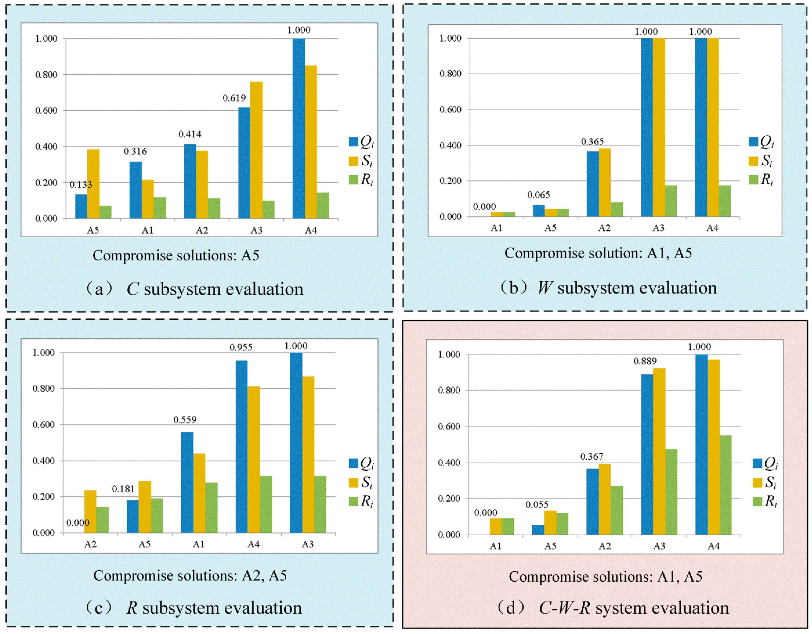
Rank the alternatives from subsystems.

Besides the whole system evaluation mentioned above, the evaluations on the three subsystems (i.e., C subsystem, W subsystem and R subsystem) are also conducted to show the performance of each alternative from different perspectives, the evaluation results are shown in Figure 6.

It can be seen from Figure 6a that A5 is the compromise solution in C subsystem evaluation, which indicates that in terms of supplier capability dimension, A5 has the strongest capability to participate in the cooperative development project. However, in Figure 6b W subsystem evaluation, A1 and A5 are the compromise solution, which indicates that in terms of the supplier willingness dimension, A1 and A5 have the stronger desire to establish a strategic partnership with the buyer. Yet, A2 and A5 are the compromise solutions in Figure 6c R subsystem evaluation, which indicates that in terms of supply risk dimension, the supply risks of A2 and A5 are relatively small, in other words, A2 and A5 are closer to the buyer. Finally, in Figure 6d C-W-R system evaluation, A1 and A5 are the compromise solutions. It can be noted that the main reason leading to the difference lies in the different weights of the three subsystems, the weight of C subsystem is 0.551, W subsystem is 0.347, and R subsystem is 0.102. Due to the large proportion of C and W subsystems, they have greater influence on the final evaluation result.

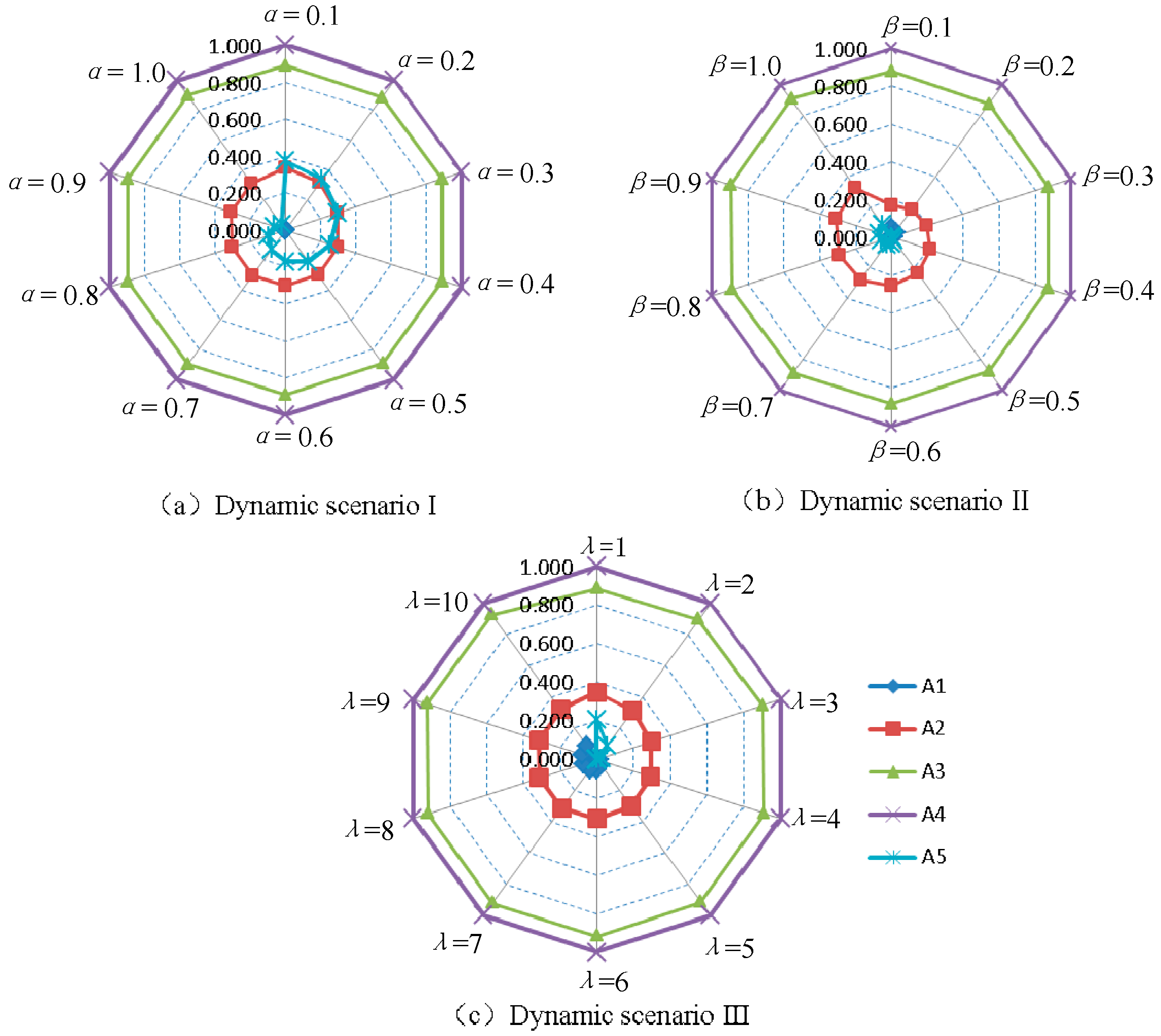
4.4. Sensitivity Analysis

In the process of MCDM, risk preference attitudes of DMs vary with each individual. To examine and verify the proposed framework’s validity and robustness, the coefficient set representing risk preferences (α, β, λ) is selected to conduct sensitivity analyses.

In the value function of PT, α represents the convexity in the gain situation and β denotes the concavity in the loss situation, α and β are adjustable coefficients satisfying the constraints 0 ≤ α, β ≤ 1, and λ describes loss aversion satisfying λ > 1 [41].

To analyze the effect of DMs’ risk attitudes on the results, there are three dynamic scenarios which are constructed by adjusting one risk parameter at a time:

• Dynamic scenario I: adjusting α from 0 to 1 and keeping β, λ constant.
• Dynamic scenario II: adjusting β from 0 to 1 and keeping α, λ constant.
• Dynamic scenario III: adjusting λ from 1 to 10 and keeping α β constant.

The results of dynamic scenario I are shown in Figure 7a, with α increasing, the Q₅ value of A5 shows a downward trend, while Q₁ value of A1 is always 0 (i.e., the optimal value) and Q₄ value of A4 is always 1 (i.e., the worst value), respectively. When α exceeds 0.4, A5 owns a smaller Q₅ value than 1/(5 − 1) and it comes to rank second, primarily because the risk of A5 is greater than that of A2 when DMs consider the gains expectations.

In dynamic scenario II as presented in Figure 7b, with β increasing, the Q₁ value of A1 shows a declining trend, the corresponding values of A2 and A5 show rising trends, while Q₄ value of A4 is always 1 (i.e., the worst value). It is worth noting that when β ≤ 0.4, the Q₅ value of alternative supplier A5 is very close to zero while when β ≥ 0.4, the Q₁ value of alternative supplier A1 is very close to zero, which implies that DMs’ psychological features towards risk seeking influences the results of alternative selections.

Figure 7c depicts the results of dynamic scenario III, since the characteristic of loss aversion effect is that the pain in the face of loss is much more than the pleasure in the face of gain, the parameter λ works in reality. In the beginning, when λ = 1, the ranking of alternatives is Q₁ < Q₅ < Q₂< Q₃ < Q₄. As λ increases, the alternative supplier A5 shows the decrease tendency in the Q₅ value, but Q₄ value of A4 is always 1 (i.e., the worst value), and while the corresponding value of A1 increase slightly. When λ = 4, Q₅ = 0 and Q₅ < Q₁, the ranking of alternatives becomes Q₅ < Q₁ < Q₂< Q₃ < Q₄, which implies that when λ increases, DMs focus more on the alternatives’ losses than the gains.

Based on the above analysis, although the Q_i values of alternative suppliers change as α, β, λ fluctuate in numerical values, Q₄ value of A4 is always 1 in most cases while the corresponding values of A1 and A5 are relatively sensitive.

4.5. Comparison Analysis

Generally, indicator weights are important in the process of decision making. To the authors’ best knowledge, previous studies rarely consider adopting triangular fuzzy judgements to convey importance comparisons in the field of supplier selection. However, it is worth noting in practice, it is difficult for experts to give an exact crisp value for the importance of indicators due to their knowledge background and cognitive style. Therefore, the triangular fuzzy linguistic judgements are integrated with BWM method in this study for determining different indicator weights. As shown in

Table 9. Results and comparison analysis.

	Fuzzy BWM-PT-VIKOR Method		Equal Indicators’ Weights-PT-VIKOR Method		Fuzzy BWM-PT-TOPSIS Method
	Qi1	Ranking	Qi2	Ranking	Li	Ranking
A1	0.000	1	0.093	2	0.968	1
A2	0.367	3	0.329	3	0.512	3
A3	0.889	4	0.899	4	0.138	4
A4	1.000	5	1.000	5	0.010	5
A5	0.055	2	0.000	1	0.786	2
Selected supplier(s)	A1, A5		A1, A5		A1

, comparison results of the proposed fuzzy BWM-PT-VIKOR method and the conventional equal indicators’ weights-PT-VIKOR method are obvious, the rankings of A1 and A5 change while the others remain unchanged. One of the reasons is that the fuzzy BWM method considers the experts judgments on the indicators’ importance degrees, while the different importance information cannot be reflected in the equal indicators’ weights method.

In addition, Technique for Order Preference by Similarity to Ideal Solution (TOPSIS) is also an MCDM technique with broad adoption as VIKOR [31], so a comparison analysis between fuzzy BWM-PT-TOPSIS method and the proposed method is also conducted. As shown in Table 9, the rankings of five alternatives remain unchanged while the selection results are different. In this perspective, A1 is the only best alternative with fuzzy BWM-PT-TOPSIS method while A1 and A5 are compromise alternatives with the proposed method in this paper, which imply that the proposed method is an effective MCDM tool. Particularly in the situations where the DMs are not able, or do not know to express preferences at the beginning of system design, the obtained compromise solutions could be the base of negotiation, involving the DMs’ preference by criteria weights.

To sum up, the proposed fuzzy BWM-PT-VIKOR method is an effective and reliable approach in MCDM problems. This method considers both aspects of the different weights of indicators and the DMs’ psychological features, so it can be employed to obtain better and more comprehensive results in real-world collaborative negotiation applications.

4.6. Managerial Suggestions

Although alternative suppliers A1 and A5 as compromise solutions performed better overall than the others, they were not perfect. Some important problems were highlighted through the indicator values in the C-W-R evaluation system and three other sub-evaluation systems. Firstly, from the perspective of the supplier capability dimension, A1 still left a lot of room for improvement. For example, as presented in Figure 8, A1 had 2546 patent applications, which was much less than those of A2 with 3033 and A5 with 2553. What is more, R&D expenditure input intensity in A1 was less than that of A2, A3, and A5, relative share of R&D employees in A1 was also less than that of A4. This implies that A1’s innovation capability still needed to be strengthened. In addition, as an important performance indicator of the power battery, the specific energy density of existing product in A1 was up to 240.56 Wh/kg, lower than A3 with 249.16 Wh/kg, and this shows that A1’s quality capability needed to be improved. Secondly, from the perspective of supplier willingness dimension, A5 had a relatively lower willingness than A1 to participate in the buyer−supplier cooperative development project, so H Company should make clear the reason for A5’s low willingness and endeavor to win preferred customer status. Thirdly, from the perspective of supply risk dimension, A1 had higher risk than A2 and A5, as depicted in Figure 8, it takes longer train hours from A1 (than all others) to H Company.

Based on the above analysis, some managerial suggestions were put forward for guiding H Company to select the innovative power battery suppliers who had highest potential to contribute to the buyer−supplier collaborative innovation.

(1) A1, as the first compromise supplier, still needs to improve its own capability constantly. For instance, through increasing R&D expenditure input intensity, employing more R&D employees and applying more patent numbers to improve the R&D capability, thereby improving the product quality of technological innovation, one of the core performance indexes of power batteries, specific energy density will be improved in the future product. From the perspective of reducing the supply risk dimension, because A1 is geographically distant from H Company, A1 could set up NEV power battery R&D centers and production bases around H Company to facilitate better communication and cooperation with H Company [24].

(2) A5, as the second compromise supplier, has strong capability while lower willingness to cooperate with H Company than A1. It is worthy of special attention from the standpoint of H Company. Two-way communication between A5 and H Company should be strengthened which would be conducive to combining their common interests, and then enhance mutual trust in business relationships [23]. In a word, H Company should take initiatives in driving supplier commitment to gain preferred customer status [55].

(3) A2, not included in the compromise suppliers, but still has its own advantages from the perspective of the supply risk dimension. According to the results of R subsystem evaluation, A2 ranks first and is one of the compromise suppliers, which implies that A2 has the lowest supply risk to cooperate with H Company. Therefore, H Company could pay close attention to A2 as a potential supplier and help it improve its own capability and willingness to cooperate with H Company through some measures, such as knowledge transfer [28], supplier incentives, etc., [35].

(4) A3 and A4, they are always in the bottom two whether from comparison analysis in Table 9, evaluation results from four perspectives in Figure 6, or sensitivity experiments in Figure 7. This indicates that both A3 and A4 do not perform well in terms of supplier capacity, supplier willingness and supply risk. Therefore, H Company can give up considering these two suppliers.

(5) H Company, as a manufacturer of NEVs and the purchaser of power batteries, should try its best to improve its own capability and develop long-term ties with capable suppliers to establish a competitive advantage in the field of NEVs [19]. Firstly, H Company can take initiatives from the buyer’s standpoint in inspiring supplier commitment to obtain a priority customer status and win the willingness of capable suppliers. Secondly, H Company should pay close attention to potential innovative suppliers and help them improve their own capability and willingness to collaborate [34]. Thirdly, H Company could reduce supply risks from the perspective of supplier development and management, such as supplier assessment and feedback [34], closing the cognitive gap [33], knowledge transfer [28], supplier incentives [35], so as to establish an innovation alliance between NEV manufacturer and the power battery suppliers for obtaining product competitive advantage in the field of NEVs.

5. Conclusions and Future Research Orientation

The main viewpoint of this paper is that NEV manufacturers and power battery suppliers should carry out cooperative development and collaborative innovation together. Therefore, a novel decision framework is proposed from the perspective of collaborative innovation for guiding on NEV manufacturers to select the innovative suppliers who have highest potential to contribute to the buyer’s innovation.

In this study, the main contributions are listed as follows: (1) a C-W-R comprehensive evaluation system with consideration of supply risk from the perspective of multi-proximity, which is closely bound up with the collaborative innovation level while only considered from geographical proximity in the previous supplier selection research, is established for innovative supplier selection. (2) Hesitant fuzzy symmetrical linguistic judgement is employed to evaluate the qualitative criteria in the indicator system, which fully depicts hesitation and fuzziness in decision-making processes. (3) The VIKOR symmetrical technique is proposed, integrating prospect theory to rank alternative suppliers. In this method, a comprehensive prospect value decision matrix with consideration of the DMs’ risk attitude is more in line with the actual process of decision-making, and the VIKOR method utilized to select compromise solution(s) but not the only optimal solution is more applicable to the situation of negotiation decision. (4) A case study was carried out in NEV manufacturers of China to certify the practicality of the evaluation methodology. Using the proposed decision framework, the five-power battery alternative suppliers A1, A2, A3, A4 and A5 received collaborative innovation potential ranking of I, III, IV, V, II. Furthermore, a comparison analysis with equal indicator weights-PT-VIKOR method and fuzzy BWM-PT-TOPSIS method was carried out to certify the validity and efficiency of the proposed framework. Finally, based on the case study, some concrete managerial suggestions were put forward from NEV manufacturers’ standpoint to identify power battery innovative suppliers who had the highest potential to contribute to the NEV manufacturers’ innovation and achieve long-term cooperative development.

The evaluation methodology proposed in this paper not only can be employed to conduct supplier selection evaluation, but also could be adapted to other MCDM problems. Besides, for the decision-making problem of cooperative development between NEV manufacturers and suppliers, since the DMs’ risk attitude varies with different individuals, introducing deep learning methods and multiagent modeling to simulate the DMs’ risk preferences could present the dynamic evolution characteristics of the model, which will be a vital research orientation in the future.

References

1. Li, W.; Long, R.; Chen, H. Consumers’ evaluation of national new energy vehicle policy in China: An analysis based on a four-paradigm model. Energy Policy 2016, 99, 33–41. [Google Scholar] [CrossRef]
2. Kendall, M. Fuel cell development for New Energy Vehicles (NEVs) and clean air in China. Prog. Nat. Sci. Mater. Int. 2018, 28, 113–120. [Google Scholar] [CrossRef]
3. Gong, H.; Wang, M.; Wang, H. New energy vehicles in China: Policies, demonstration and progress. Mitig. Adapt. Strat. Glob. Chang. 2013, 18, 207–228. [Google Scholar] [CrossRef]
4. Kimble, C.; Wang, H. China’s new energy vehicles: Value and innovation. J. Bus. Strategy 2013, 34, 13–20. [Google Scholar] [CrossRef] [Green Version]
5. China’s Production and Sales of New Energy Vehicles Ranked First in the World for Five Consecutive Years 2020. Available online: http://www.gov.cn/xinwen/2020-10/09/content_5549829.htm (accessed on 10 October 2020). (In Chinese)
6. The National Power Battery Innovation Center Was Established 2016. Available online: http://www.gov.cn/xinwen/2016-06/30/content_5087182.htm (accessed on 1 July 2020). (In Chinese)
7. Wang, X.; Song, Y.; Xia, W.; Liu, H.; Yang, S. Promoting the development of the new energy automobile industry in China: Technology selection and evaluation perspective. J. Renew. Sustain. Energy 2018, 10, 045901. [Google Scholar] [CrossRef]
8. Zhao, H.; Guo, S.; Zhao, H. Comprehensive assessment for battery energy storage systems based on fuzzy-MCDM considering risk preferences. Energy 2019, 168, 450–461. [Google Scholar] [CrossRef]
9. Zeng, Z.; Liu, X.; Jiang, X.; Liu, Z.; Peng, Z.; Feng, X.; Chen, W.; Xia, D.; Ai, X.; Yang, H.; et al. Enabling an intrinsically safe and high-energy-density 4.5 V-class Li-ion battery with nonflammable electrolyte. InfoMat 2020, 2, 984–992. [Google Scholar] [CrossRef]
10. Huth, C.; Kieckhäfer, K.; Spengler, T.S. Make-or-buy strategies for electric vehicle batteries—A simulation-based analysis. Technol. Forecast. Soc. Chang. 2015, 99, 22–34. [Google Scholar] [CrossRef]
11. Fan, Z.P.; Chen, Z.; Zhao, X. Battery outsourcing decision and product choice strategy of an electric vehicle manufacturer. Int. Trans. Oper. Res. 2020. [Google Scholar] [CrossRef]
12. Luzzini, D.; Amann, M.; Caniato, F.; Essig, M. The path of innovation: Purchasing and supplier involvement into new product development. Ind. Mark. Manag. 2015, 47, 109–120. [Google Scholar] [CrossRef]
13. Le, M.; Merminod, V.; Yager, M. Collaborative practices in new product development projects involving suppliers. Prod. Plan. Control 2020, 31, 308–321. [Google Scholar] [CrossRef]
14. Wang, C.N.; Viet, V.T.H.; Ho, T.P.; Nguyen, T.V.; Nguyen, T.V. Multi-Criteria Decision Model for the Selection of Suppliers in the Textile Industry. Symmetry 2020, 12, 979. [Google Scholar] [CrossRef]
15. Dickson, G. An analysis of vendor selection systems and decisions. J. Purch. 1966, 2, 5–17. [Google Scholar] [CrossRef]
16. Kraljic, P. Purchasing must become supply management. Harv. Bus. Rev. 1983, 61, 109–117. [Google Scholar]
17. Weber, C.; Current, J.; Benton, W. Vendor selection criteria and methods. Eur. J. Oper. Res. 1991, 50, 2–18. [Google Scholar] [CrossRef]
18. Hoetker, G. How much you know versus how well I know you: Selecting a supplier for a technically innovative component. Strateg. Manag. J. 2005, 26, 75–96. [Google Scholar] [CrossRef]
19. Meksavang, P.; Shi, H.; Lin, S.; Liu, H. An extended picture fuzzy VIKOR approach for sustainable supplier management and its application in the beef industry. Symmetry 2019, 11, 468. [Google Scholar] [CrossRef] [Green Version]
20. Sinha, A.; Anand, A. Development of sustainable supplier selection index for new product development using multi criteria decision making. J. Clean. Prod. 2018, 197, 1587–1596. [Google Scholar] [CrossRef]
21. Kaufman, A.; Wood, C.; Theyel, G. Collaboration and technology linkages: A strategic supplier typology. Strateg. Manag. J. 2000, 21, 649–663. [Google Scholar] [CrossRef]
22. Govindan, K.; Rajendran, S.; Sarkis, J.; Murugesan, P. Multi criteria decision making approaches for green supplier evaluation and selection: A literature review. J. Clean. Prod. 2015, 98, 66–83. [Google Scholar] [CrossRef]
23. Pulles, J.; Veldman, J.; Schiele, H. Identifying innovative suppliers in business networks: An empirical study. Ind. Mark. Manag. 2014, 43, 409–418. [Google Scholar] [CrossRef]
24. Schiele, H. How to distinguish innovative suppliers? Identifying innovative suppliers as new task for purchasing. Ind. Mark. Manag. 2006, 35, 925–935. [Google Scholar] [CrossRef] [Green Version]
25. Upadhyay, A.; Baglieri, E. Innovative supplier selection: Key success factors. Int. J. Innov. Bus. 2012, 1, 336–344. Available online: http://sure.sunderland.ac.uk/id/eprint/3951 (accessed on 8 August 2020).
26. Rese, M. Successful and sustainable business partnerships: How to select the right partners. Ind. Mark. Manag. 2006, 35, 72–82. [Google Scholar] [CrossRef]
27. Zsidisin, G.A. A grounded definition of supply risk. J. Purch. Supply Manag. 2003, 9, 217–224. [Google Scholar] [CrossRef]
28. Knoben, J.; Oerlemans, L. Proximity and inter organizational collaboration: A literature review. Int. J. Manag. Rev. 2006, 8, 71–89. [Google Scholar] [CrossRef] [Green Version]
29. Nooteboom, B.; Haverbeke, W.V.; Duysters, G.; Gilsing, V.; Oord, A. Optimal cognitive distance and absorptive capacity. Res. Policy 2007, 36, 1016–1034. [Google Scholar] [CrossRef] [Green Version]
30. Opricovic, S.; Tzeng, G. Compromise solution by MCDM methods: A comparative analysis of VIKOR and TOPSIS. Eur. J. Oper. Res. 2004, 156, 445–455. [Google Scholar] [CrossRef]
31. Opricovic, S.; Tzeng, G. Extended VIKOR method in comparison with outranking methods. Eur. J. Oper. Res. 2007, 178, 514–529. [Google Scholar] [CrossRef]
32. Rezaei, J. Best-worst multi-criteria decision-making method. Omega 2015, 53, 49–57. [Google Scholar] [CrossRef]
33. Rezaei, J. Best-worst multi-criteria decision-making method: Some properties and a linear model. Omega 2016, 64, 126–130. [Google Scholar] [CrossRef]
34. Rezaei, J.; Ortt, R. A multi-variable approach to supplier segmentation. Int. J. Prod. Res. 2012, 50, 4593–4611. [Google Scholar] [CrossRef] [Green Version]
35. Rezaei, J.; Wang, J.; Tavasszy, L. Linking supplier development to supplier segmentation using Best Worst Method. Expert Syst. Appl. 2015, 42, 9152–9164. [Google Scholar] [CrossRef]
36. Garg, C.P.; Sharma, A. Sustainable outsourcing partner selection and evaluation using an integrated BWM–VIKOR framework. Environ. Dev. Sustain. 2020, 22, 1529–1557. [Google Scholar] [CrossRef]
37. Kahneman, D.; Tversky, A. Prospect theory: An analysis of decision under risk. In Handbook of the Fundamentals of Financial Decision Making; World Scientific: Singapore, 2013; pp. 99–127. [Google Scholar] [CrossRef] [Green Version]
38. Tversky, A.; Kahneman, D. Advances in prospect theory: Cumulative representation of uncertainty. J. Risk Uncertain. 1992, 5, 297–323. [Google Scholar] [CrossRef]
39. Wu, Y.; Ke, Y.; Xu, C.; Li, L. An integrated decision-making model for sustainable photovoltaic module supplier selection based on combined weight and cumulative prospect theory. Energy 2019, 181, 1235–1251. [Google Scholar] [CrossRef]
40. Wu, Y.; Xu, C.; Zhang, T. Evaluation of renewable power sources using a fuzzy MCDM based on cumulative prospect theory: A case in China. Energy 2018, 147, 1227–1239. [Google Scholar] [CrossRef]
41. Qin, J.; Liu, X.; Pedrycz, W. An extended VIKOR method based on prospect theory for multiple attribute decision making under interval type-2 fuzzy environment. Knowl.-Based Syst. 2015, 86, 116–130. [Google Scholar] [CrossRef]
42. Tu, Y.; Chen, K.; Wang, H.; Li, Z. Regional water resources security evaluation based on a hybrid fuzzy BWM-TOPSIS method. Int. J. Environ. Res. Public Health 2020, 17, 4987. [Google Scholar] [CrossRef]
43. Li, Z.; Zhang, Q.; Liao, H. Efficient-equitable-ecological evaluation of regional water resource coordination considering both visible and virtual water. Omega 2019, 83, 223–235. [Google Scholar] [CrossRef]
44. Liu, Y.; Li, L.; Tu, Y.; Mei, Y. Fuzzy TOPSIS-EW Method with Multi-Granularity Linguistic Assessment Information for Emergency Logistics Performance Evaluation. Symmetry 2020, 12, 1331. [Google Scholar] [CrossRef]
45. Guo, S.; Zhao, H. Fuzzy best-worst multi-criteria decision-making method and its applications. Knowl.-Based Syst. 2017, 121, 23–31. [Google Scholar] [CrossRef]
46. Liao, H.; Xu, Z.; Zeng, X. Hesitant fuzzy linguistic VIKOR method and its application in qualitative multiple criteria decision making. IEEE Trans. Fuzzy Syst. 2014, 23, 1343–1355. [Google Scholar] [CrossRef]
47. Liao, H.; Xu, Z.; Zeng, X. Distance and similarity measures for hesitant fuzzy linguistic term sets and their application in multi-criteria decision making. Inf. Sci. 2014, 271, 125–142. [Google Scholar] [CrossRef]
48. Harland, C.; Brenchley, R.; Walker, H. Risk in supply networks. J. Purch. Supply Manag. 2003, 9, 51–62. [Google Scholar] [CrossRef]
49. Guertler, B.; Spinler, S. When does operational risk cause supply chain enterprises to tip? A simulation of intra-organizational dynamics. Omega 2015, 57, 54–69. [Google Scholar] [CrossRef]
50. Boschma, R. Proximity and innovation: A critical assessment. Reg. Stud. 2005, 39, 61–74. [Google Scholar] [CrossRef]
51. Davids, M.; Frenken, K. Proximity, knowledge base and the innovation process: Towards an integrated framework. Reg. Stud. 2018, 52, 23–34. [Google Scholar] [CrossRef] [Green Version]
52. Caragliu, A.; Nijkamp, P. Space and knowledge spillovers in European regions: The impact of different forms of proximity on spatial knowledge diffusion. J. Econ. Geogr. 2016, 16, 749–774. [Google Scholar] [CrossRef]
53. Choi, T.Y.; Hartley, J.L. An exploration of supplier selection practices across the supply chain. J. Oper. Manag. 1996, 14, 333–343. [Google Scholar] [CrossRef]
54. Kannan, V.R.; Tan, K.C. Supplier selection and assessment: Their impact on business performance. J. Supply Chain Manag. 2002, 38, 11–21. [Google Scholar] [CrossRef] [Green Version]
55. Patrucco, A.; Moretto, A.; Luzzini, D.; Glasy, A. Obtaining supplier commitment: Antecedents and performance outcomes. Int. J. Prod. Econ. 2020, 220, 107449. [Google Scholar] [CrossRef]
Figure 1. (a) Nomenclature of suppliers; (b) “Capability” and “Willingness” dimensions; (c) Exacted “Supply risk” dimension; (d) Three dimensions of innovative supplier evaluation.
Symmetry 13 00143 g001
Figure 2. Innovative supplier evaluation C-W-R system.
Symmetry 13 00143 g002
Figure 3. Framework of BWM-PT-VIKOR method integrating fuzzy linguistic judgement.
Symmetry 13 00143 g003
Figure 4. Examples of hesitant fuzzy linguistic judgements.
Symmetry 13 00143 g004
Figure 5. Location of the study enterprises.
Symmetry 13 00143 g005
Figure 6. Evaluation results from four perspectives.
Symmetry 13 00143 g006
Figure 7. Spider diagrams of sensitivity analysis.
Symmetry 13 00143 g007
Figure 8. Situations of some indicators.
Symmetry 13 00143 g008