Symmetry, Transactions, and the Mechanism of Wave Function Collapse

Abstract

The Transactional Interpretation of quantum mechanics exploits the intrinsic time-symmetry of wave mechanics to interpret the $\psi$ and $\psi$* wave functions present in all wave mechanics calculations as representing retarded and advanced waves moving in opposite time directions that form a quantum “handshake” or transaction. This handshake is a 4D standing-wave that builds up across space-time to transfer the conserved quantities of energy, momentum, and angular momentum in an interaction. Here, we derive a two-atom quantum formalism describing a transaction. We show that the bi-directional electromagnetic coupling between atoms can be factored into a matched pair of vector potential Green’s functions: one retarded and one advanced, and that this combination uniquely enforces the conservation of energy in a transaction. Thus factored, the single-electron wave functions of electromagnetically-coupled atoms can be analyzed using Schrödinger’s original wave mechanics. The technique generalizes to any number of electromagnetically coupled single-electron states—no higher-dimensional space is needed. Using this technique, we show a worked example of the transfer of energy from a hydrogen atom in an excited state to a nearby hydrogen atom in its ground state. It is seen that the initial exchange creates a dynamically unstable situation that avalanches to the completed transaction, demonstrating that wave function collapse, considered mysterious in the literature, can be implemented with solutions of Schrödinger’s original wave mechanics, coupled by this unique combination of retarded/advanced vector potentials, without the introduction of any additional mechanism or formalism. We also analyze a simplified version of the photon-splitting and Freedman–Clauser three-electron experiments and show that their results can be predicted by this formalism.

1. Introduction

Quantum mechanics (QM) was never properly finished. Instead, it was left in an exceedingly unsatisfactory state by its founders. Many attempts by highly qualified individuals to improve the situation have failed to produce any consensus about either (a) the precise nature of the problem, or (b) what a better form of QM might look like.

At the most basic level, a simple observation illustrates the central conceptual problem:

An excited atom somewhere in the universe transfers all of its excitation energy to another single atom, independent of the presence of the vast number of alternative atoms that could have received all or part of the energy. The obvious “photon-as-particle” interpretation of this situation has a one-way symmetry: The excited source atom is depicted as emitting a particle, a photon of electromagnetic energy that is somehow oscillating with angular frequency $\omega$ while moving in a particular direction. The photon is depicted as carrying a quantum of energy $\hslash \omega$, a momentum $\hslash \omega /c$, and an angular momentum ℏ through space, until it is later absorbed by some unexcited atom. The emission and absorption are treated as independent isolated events without internal structure. It is insisted that the only real and meaningful quantities describing this process are probabilities, since these are measurable. The necessarily abrupt change in the quantum wave function of the system when the photon arrives (and an observer potentially gains information) is called “wave function collapse” and is considered to be a mysterious process that the founders of QM found it necessary to “put in by hand” without providing any mechanism. [The missing mechanism behind wave function collapse is sometimes called “the measurement problem”, particularly by acolytes of Heisenberg’s knowledge interpretation. In our view, measurement requires wave function collapse but does not cause it.] [Side comments will be put in square brackets]

Referring to statistical quantum theory, which is reputed to apply only to ensembles of similar systems, Albert Einstein [1] had this to say:

“I do not believe that this fundamental concept will provide a useful basis for the whole of physics.”

“I am, in fact, firmly convinced that the essentially statistical character of contemporary quantum theory is solely to be ascribed to the fact that this [theory] operates with an incomplete description of physical systems.”

“One arrives at very implausible theoretical conceptions, if one attempts to maintain the thesis that the statistical quantum theory is in principle capable of producing a complete description of an individual physical system …”

“Roughly stated, the conclusion is this: Within the framework of statistical quantum theory, there is no such thing as a complete description of the individual system. More cautiously, it might be put as follows: The attempt to conceive the quantum-theoretical description as the complete description of the individual systems leads to unnatural theoretical interpretations, which become immediately unnecessary if one accepts the interpretation that the description refers to ensembles of systems and not to individual systems. In that case, the whole ’egg-walking’ performed in order to avoid the ’physically real’ becomes superfluous. There exists, however, a simple psychological reason for the fact that this most nearly obvious interpretation is being shunned—for, if the statistical quantum theory does not pretend to describe the individual system (and its development in time) completely, it appears unavoidable to look elsewhere for a complete description of the individual system. In doing so, it would be clear from the very beginning that the elements of such a description are not contained within the conceptual scheme of the statistical quantum theory. With this. one would admit that, in principle, this scheme could not serve as the basis of theoretical physics. Assuming the success of efforts to accomplish a complete physical description, the statistical quantum theory would, within the framework of future physics, take an approximately analogous position to the statistical mechanics within the framework of classical mechanics. I am rather firmly convinced that the development of theoretical physics will be of this type, but the path will be lengthy and difficult.”

“If it should be possible to move forward to a complete description, it is likely that the laws would represent relations among all the conceptual elements of this description which, per se, have nothing to do with statistics.”

In what follows we put forth a simple approach to describing the individual system (and its development in time), which Einstein believed was missing from statistical quantum theory and which must be present before any theory of physics could be considered to be complete.

The way forward was suggested by the phenomenon of entanglement. Over the past few decades, many increasingly exquisite Einstein–Podolsky–Rosen [2] (EPR) experiments [3,4,5,6,7,8,9,10,11] have demonstrated that multi-body quantum systems with separated components that are subject to conservation laws exhibit a property called “quantum entanglement” [12]: Their component wave functions are inextricably locked together, and they display a nonlocal correlated behavior enforced over an arbitrary interval of space-time without any hint of an underlying mechanism or any show of respect for our cherished classical “arrow of time”. Entanglement is the most mysterious of the many so-called “quantum mysteries”.

It has thus become clear that the quantum transfer of energy must have quite a different symmetry from that implied by this simple “photon-as-particle” interpretation. Within the framework of statistical QM, the intrinsic symmetry of the energy transfer and the mechanisms behind wave function collapse and entanglement have been greatly clarified by the Transactional Interpretation of quantum mechanics (TI), developed over several decades by one of us and recently described in some detail in the book The Quantum Handshake [12]. [We note that Ruth Kastner has extended her “probabilist” variant of the TI, which embraces the Heisenberg/probability view and characterizes transactions as events in many-dimensional Hilbert space, into the quantum-relativistic domain [13,14] and has used it to extend and enhance the “decoherence” approach to quantum interpretation [15].

This paper begins with a tutorial review of the TI approach to a credible photon mechanism developed in the book Collective Electrodynamics [16], followed by a deeper dive into the electrodynamics of the quantum handshake, and finally includes descriptions of several historic experiments that have excluded entire classes of theories. We conclude that the approach described here has not been excluded by any experiment to date.

1.1. Wheeler–Feynman Electrodynamics

The Transactional Interpretation was inspired by classical time-symmetric Wheeler–Feynman electrodynamics [17,18] (WFE), sometimes called “absorber theory”. Basically, WFE assumes that electrodynamics must be time-symmetric, with equally valid retarded waves (that arrive after they are emitted) and advanced waves (that arrive before they are emitted). WFE describes a “handshake” process accounting for emission recoil in which the emission of a retarded wave stimulates a future absorber to produce an advanced wave that arrives back at the emitter at the instant of emission. WFE is based on electrodynamic time symmetry and has been shown to be completely interchangeable with conventional classical electrodynamics in its predictions.

WFE asserts that the breaking of the intrinsic time-symmetry to produce the electromagnetic arrow of time, i.e., the observed dominance of retarded radiation and absence of advanced radiation in the universe, arises from the presence of more absorption in the future than in the past. In an expanding universe, that assertion is questionable. One of us has suggested an alternative cosmological explanation [19], which employs advanced-wave termination and reflection from the singularity of the Big Bang.

1.2. The Transactional Interpretation of Quantum Mechanics

The Transactional Interpretation of quantum mechanics [12] takes the concept of a WFE handshake from the classical regime into the quantum realm of photons and massive particles. The retarded and advanced waves of WFE become the quantum wave functions $\psi$ and $\psi$*. Note that the complex conjugation of $\psi$* is in effect the application of the Wigner time-reversal operator, thus representing an advanced wave function that carries negative energy from the present to the past.

Let us here clarify what an interpretation of quantum mechanics actually is. An interpretation serves the function of explaining and clarifying the formalism and procedures of its theory. In our view, the mathematics is (and should be) exclusively contained in the formalism itself. The interpretation should not introduce additional variant formalism. [We note, however, that this principle is violated by the Bohm–de Broglie “interpretation” with its “quantum potentials” and uncertainty-principle-violating trajectories, by the Ghirardi–Rimini–Weber “interpretation” with its nonlinear stochastic term, and by many other so-called interpretations that take the questionable liberty of modifying the standard QM formalism. In that sense, these are alternative variant quantum theories, not interpretations at all.]

The present work is a calculation describing the formation of a transaction that was inspired by the Transactional Interpretation but has not previously been a part of it. In Section 12 below, we discuss how the TI is impacted by this work. We use Schrödinger’s original wave mechanics formalism with the inclusion of retarded and advanced electromagnetic four-potentials to describe and illuminate the processes of transaction formation and the collapse of the wave function. We show that this approach can provide a detailed mathematical description of a “quantum-jump” in which what seems to be a photon is emitted by one hydrogen atom in an excited state and excites another hydrogen atom initially in its ground state. Thus, the mysterious process of wave function collapse becomes just a phenomenon involving an exchange of advanced/retarded electromagnetic waves between atomic wave functions described by the Schrödinger formalism.

As illustrated schematically in Figure 1, the process described involves the initial existence in each atom of a very small admixture of the wave function for the opposite state, thereby forming two-component states in both atoms. This causes them to become weak dipole radiators oscillating at the same difference-frequency ${\omega }_0$. The interaction that follows, characterized by a retarded-advanced exchange of 4-vector potentials, leads to an exponential build-up of a transaction, resulting in the complete transfer of one photon worth of energy $\hslash {\omega }_0$ from one atom to the other. This process is described in more detail below.

2. Physical Mechanism of the Transfer

The standard formalism of QM consists of a set of arbitrary rules, conventionally viewed as dealing only with probabilities. When illuminated by the TI, that formalism hints at an underlying physical mechanism that might be understood, in the usual sense of the concept understood. The first glimpse of such an understanding, and of the physical nature of the transactional symmetry, was suggested by Gilbert N. Lewis in 1926 [20,21], the same year he gave electromagnetic energy transfer the name “photon”:

“It is generally assumed that a radiating body emits light in every direction, quite regardless of whether there are near or distant objects which may ultimately absorb that light; in other words that it radiates ’into space’…”

“I am going to make the contrary assumption that an atom never emits light except to another atom…”

“I propose to eliminate the idea of mere emission of light and substitute the idea of transmission, or a process of exchange of energy between two definite atoms… Both atoms must play coordinate and symmetrical parts in the process of exchange…”

“In a pure geometry it would surprise us to find that a true theorem becomes false when the page upon which the figure is drawn is turned upside down. A dissymmetry alien to the pure geometry of relativity has been introduced by our notion of causality.”

In what follows, we demonstrate that the pair of coupled Schrödinger equations describing the two atoms, as coupled by a relativistically correct description of the electromagnetic field, exhibit a unique solution. This solution has exactly the symmetry of the TI and thus provides a physically understandable mechanism for the experimentally observed behavior: Both atoms, in the words of Lewis, “play coordinate and symmetrical parts in the process of exchange”.

The solution gives a smooth transition in each of the atomic wave functions, brought to abrupt closure by the highly nonlinear increase in coupling as the transition proceeds. The origin of statistical behavior and “quantum randomness” can be understood in terms of the random distribution of wave-function amplitudes and phases provided by the perturbations of the many other potential recipient atoms; no “hidden variables” are required. Although much remains to be done, these findings might be viewed as a next step towards a physical understanding of the process of quantum energy transfer.

We will close by indicating the deep, fundamental questions that we have not addressed, and that must be understood before anything like a complete physical understanding of QM is in hand.

3. Quantum States

In 1926, Schrödinger, seeking a wave-equation description of a quantum system with mass, adopted Planck’s notion that energy was somehow proportional to frequency together with deBroglie’s idea that momentum was the propagation vector of a wave and crafted his wave equation for the time evolution of the wave function $\Psi$ [22]:

$$-\frac{\hslash }{2mi}{\nabla }^2\Psi +\frac{qV}{i\hslash }\Psi =\frac{\partial \Psi }{\partial t}.$$

(1)

Here, V is the electrical potential, m is the electron mass, and q is the (negative) charge on the electron. Thus, what is the meaning of the wave function $\Psi$ that is being characterized? In modern treatments, $\Psi$ is called a “probability amplitude”, which has only a probabilistic interpretation. In what follows, however, we return to Schrödinger’s original vision, which provides a detailed physical picture of the wave function and how it interacts with other charges:

“The hypothesis that we have to admit is very simple, namely that the square of the absolute value of Ψ is proportional to an electric density, which causes emission of light according to the laws of ordinary electrodynamics.”

That vision has inspired generations of talented conceptual thinkers to invent solutions to technical problems using Schrödinger’s approach. Foremost among these was Ed Jaynes who, with a number of students and collaborators, attacked a host of quantum problems in this manner [23,24,25,26,27,28,29,30]. A great deal of physical understanding was obtained, in particular concerning lasers and the coherent optics made possible by them. The theory evolved rapidly and had an enabling role in the explosive progress of that field. Indeed, the continued rapid technical progress into the present is due, in no small part, to the understanding gained through application of the Jaynes way of thinking. A detailed review of the progress up to 1972 was reported in a conference that year [30]. By then this class of theory was called neoclassical (NCT) because of its use of Maxwell’s equations. While there was no question about the utility of NCT in the conceptualization and technical realization of amazing quantum-optics devices and their application, there was a deep concern about whether it could possibly be correct at the fundamental level—maybe it was just a clever bunch of hacks. The tension over this concern was a major focus of the 1972 Third Rochester Conference on Coherence and Quantum Optics [31], and several experiments testing NCT predictions were discussed there by Jaynes [30].

He ended his presentation this way:

“We have not commented on the beautiful experiment reported here by Clauser [32], which opens up an entirely new area of fundamental importance to the issues facing us…”

“What it seems to boil down to is this: a perfectly harmless looking experimental fact (nonoccurence of coincidences at 90°), which amounts to determining a single experimental point—and with a statistical measurement of unimpressive statistical accuracy—can, at a single stroke, throw out a whole infinite class of alternative theories of electrodynamics, namely all local causal theories.”

“…if the experimental result is confirmed by others, then this will surely go down as one of the most incredible intellectual achievements in the history of science, and my own work will lie in ruins.”

The experiment he was alluding to was that of Freedman and Clauser [6], and in particular to their observaton of an essentially zero coincidence rate with crossed polarizers. The Freedman–Clauser experiment (see Section 13.3 below), with its use of entangled photon pairs, was the vanguard of an entire new direction in quantum physics that now goes under the rubric of Tests of Bell’s Inequality [3,4] and/or EPR experiments [6,7,8,9,10,11]. Both the historic EPR experiment and its analysis have been repeated many times with ever-increasing precision, and always with the same outcome: a difinitive violaton of Bell’s inequalities. Local causal theories were dead! [Much of the literature on violations of Bell’s inequalities in EPR experiments has unfortunately emphasized the refutation of local hidden-variable theories. In our view, this is a regrettable historical accident attributable to Bell. Nonlocal hidden-variable theories have been shown to be compatible with EPR results. It is locality that has been refuted. Entangled systems exhibit correlations that can only be accomodated by quantum nonlocality. The TI supplies the mechanism for that nonlocality.]

In fact, it was the manifest quantum nonlocality evident in the early EPR experiments of the 1970s that led to the synthesis of the transactional interpretation in the 1980s [19,33,34], designed to compactly explain entanglement and nonlocality. This in turn led to the search for an underlying transaction mechanism, as reported in 2000 in Collective Electrodynamics [16]. As we detail below, the quantum handshake, as mediated by advanced/retarded electromagnetic four-potentials, provides the effective non-locality so evident in modern versions of these EPR experiments. In Section 13, we analyze the Freedman–Clauser experiment in detail and show that their result is a natural outcome of our approach. Jaynes’ work does not lie in ruins—all that it needed for survival was the non-local quantum handshake! What follows is an extension and modification of NCT using a different non-Maxwellian form of E&M [16] and including our non-local Transactional approach. We illustrate the approach with the simplest possible physical arrangements, described with the major goal of conceptual understanding rather than exhaustion. Obviously, much more work needs to be done, which we point out where appropriate.

Atoms

We will begin by visualizing the electron as Schrödinger and Jaynes did: as having a smooth charge distribution in three-dimensional space, whose density is given by ${\Psi }^{*}\Psi$. There is no need for statistics and probabilities at any point in these calculations, and none of the quantities have statistical meaning. The probabilistic outcome of quantum experiments has the same origin as it does in all other experiments—random perturbations beyond the control of the experimenter. We return to the topic of probability after we have established the nature of the transaction.

For a local region of positive potential V, for example near a positive proton, the negative electron’s wave function has a local potential energy ($qV$) minimum in which the electron’s wave function can form local bound states. The spatial shape of the wave function amplitude is a trade-off between getting close to the proton, which lowers its potential energy, and bunching together too much, which increases its ${\nabla }^2$ “kinetic energy.” Equation (1) is simply a mathematical expression of this trade-off, a statement of the physical relation between mass, energy, and momentum in the form of a wave equation.

A discrete set of states called eigenstates are standing-wave solutions of Equation (1) and have the form $\Psi =R{e}^{-i\omega t}$, where R and V are functions of only the spatial coordinates, and the angular frequency $\omega$ is itself independent of time. For the hydrogen atom, the potential $V={ϵ}_0{q}_p/r$, where $q_p$ is the positive charge on the nucleus, equal in magnitude to the electron charge q. Two of the lowest-energy solutions to Equation (1) with this potential are:

$$\begin{array}{cc}\hfill {\Psi }_{100}& =\frac{e^{-r}}{\sqrt{\pi }}{e}^{-i{\omega }_{1}t}{\Psi }_{210}=\frac{r{e}^{-r/2}cos\left(\theta \right)}{4\sqrt{6\pi }}{e}^{-i{\omega }_{2}t},\hfill \end{array}$$

(2)

where the dimensionless radial coordinate r is the radial distance divided by the Bohr radius $a_0$:

$$\begin{array}{c}\hfill a_0\equiv \frac{4\pi {ϵ}_0{\hslash }^2}{m{q}^2}=0.0529\mathrm{nm},\end{array}$$

(3)

and $\theta$ is the azimuthal angle from the North Pole ($+z$ axis) of the spherical coordinate system.

The spatial “shape” of the two lowest energy eigenstates for the hydrogen atom is shown in Figure 2. Here, we focus on the excited-state wave function ${\Psi }_{210}$ that has no angular momentum projection on the z-axis. For the moment, we set aside the wave functions ${\Psi }_{21\pm 1}$, which have $+1$ and $-1$ angular momentum z-axis projections. Because, for any single eigenstate, the electron density is ${\Psi }^{*}\Psi =R{e}^{i\omega t}R{e}^{-i\omega t}=R^2$, the charge density is not a function of time, so none of the other properties of the wave function change with time. The individual eigenstates are thus stationary states. The lowest energy bound eigenstate for a given form of potential minimum is called its ground state, shown on the left in Figure 3. The corresponding charge densities are shown in Figure 4.

In 1926, Schrödinger had already derived the energies and wave functions for the stationary solutions of his equation for the hydrogen atom. His physical insight that the absolute square ${\Psi }^{*}\Psi$ of the wave function was the electron density had enabled him to work out the energy shifts of these levels caused by external applied electric and magnetic fields, the expected strengths of the transitions between pairs of energy levels, and the polarization of light from certain transitions.

These predictions could be compared directly with experimental data, which had been previously observed but not understood. He reported that these calculations were:

“…not at all difficult, but very tedious. In spite of their tediousness, it is rather fascinating to see all the well-known but not understood “rules” come out one after the other as the result of familiar elementary and absolutely cogent analysis, like e.g. the fact that ${\int }_0^{2\pi }cosm\varphi cosn\varphi d\varphi$ vanishes unless $n=m$. Once the hypothesis about ${\Psi }^{*}\Psi$ has been made, no accessory hypothesis is needed or is possible; none could help us if the “rules” did not come out correctly. However, fortunately they do [22,35].”

The Schrödinger/Jaynes approach enables us to describe continuous quantum transitions in an intuitively appealing way: We extend the electromagnetic coupling described in Collective Electrodynamics [16] to the wave function of a single electron, and require only the most rudimentary techniques of Schrödinger’s original quantum theory.

4. The Two-State System

The first two eigenstates of the Hydrogen atom, from Equation (2), form an ideal two-state system.

We refer to the 100 ground state as State 1, with wave function ${\Psi }_1$ and energy $E_1$, and to the 210 excited state as State 2, with wave function ${\Psi }_2$ and energy $E_2>E_1$:

$${\Psi }_1=R_1{e}^{-i{\omega }_{1}t}{\Psi }_2=R_2{e}^{-i{\omega }_{2}t},$$

(4)

where ${\omega }_1=E_1/\hslash$, ${\omega }_2=E_2/\hslash$, and $R_1$ and $R_2$ are real, time-independent functions of the space coordinates. The wave functions represent totally continuous matter waves, and all of the usual operations involving the wave function are methods for computing properties of this continuous distribution. The only particularly quantal assumption involved is that the wave function obeys a normalization condition:

$$\int {\Psi }^{*}\Psi d\mathrm{vol}=1,$$

(5)

where the integral is taken over the entire three-dimensional volume where $\Psi$ is non-vanishing. [Envelope functions like $R_1$ and $R_2$ generally die out exponentially with distance sufficiently far from the “region of interest,” such as an atom. Integrals like this one and those that follow in principle extend to infinity but in practice are taken out far enough that the part being neglected is within the tolerance of the calculation.].

Equation (5) ensures that the total charge will be a single electronic charge, and the total mass will be a single electronic mass.

By construction, the eigenstates of the Schrödinger equation are real and orthogonal:

$$\begin{array}{c}\hfill \int R_1{R}_{2}d\mathrm{vol}=0.\end{array}$$

(6)

The first moment $〈z〉$ of the electron distribution along the atom’s z-axis is:

$$〈z〉\equiv \int {\Psi }^{*}z\Psi d\mathrm{vol},$$

(7)

In statistical treatments, $〈z〉$ would be called the “expectation value of z”, whereas for our continuous distribution it is called the “average value of z” or the “first moment of z.” The electron wave function is a wave packet and is subject to all the Fourier properties of one, as treated at some length in Ref. [12]. Statistical QM insisted that electrons were “point particles”, so one was no longer able to visualize how they could exhibit interference or other wave properties, so a set of rules was constructed to make the outcomes of statistical experiments come out right. Among these was the uncertainty principle, which simply restated the Fourier properties of an object described by waves in a statistical context. No statistical attributes are attached to any properties of the wave function in this treatment.

Equation (7) gives the position of the center of negative charge of the electron wave function relative to the positive charge on the nucleus. When multiplied by the electronic charge q, it is called the electric dipole moment $q〈z〉$ of the charge distribution of the atom:

$$q〈z〉=q\int {\Psi }^{*}z\Psi d\mathrm{vol}.$$

(8)

From Equations (7) and (4), the dipole moment for the ith eigenstate is:

$$q〈z_i〉=q\int {\Psi }_i^{*}z{\Psi }_{i}d\mathrm{vol}=q\int R_i^{*}z{R}_{i}d\mathrm{vol}=q\int R_i^{2}zd\mathrm{vol}.$$

(9)

Pure eigenstates of the system will have a definite parity, i.e., they will have wave functions with either even symmetry [$\Psi \left(z\right)=\Psi (-z)$], or odd symmetry [$\Psi \left(z\right)=-\Psi (-z)$]. For either symmetry, the integral over $R^{2}z$ vanishes, and the dipole moment is zero. We note that, even if the wave function did not have even or odd symmetry, the dipole moment, and all higher moments as well, would be independent of time. By their very nature, eigenstates are stationary states and can be visualized as standing-waves—none of their physical spatial attributes can be functions of time. In order to radiate electromagnetic energy, the charge distribution must change with time.

The notion of stationarity is the quantum answer to the original question about atoms depicted as electrons orbiting a central nucleus like a tiny Solar System:

Why doesn’t the electron orbiting the nucleus radiate its energy away?

In his 1917 book, The Electron, R.A. Millikan [36] anticipates the solution in his comment about the

”…apparent contradiction involved in the non-radiating electronic orbit—a contradiction which would disappear, however, if the negative electron itself, when inside the atom, were a ring of some sort, capable of expanding to various radii, and capable, only when freed from the atom, of assuming essentially the properties of a point charge.”

Millikan was the first researcher to directly observe and measure the quantized charge on the electron with his famous oil-drop experiment, for which he later received the Nobel prize. Ten years before the statistical quantum theory was put in place, he had clearly seen that a continuous, symmetric electronic charge distribution would not radiate, and that the real problem was the assumption of a point charge.

5. Transitions

The eigenstates of the system form a complete basis set, so any behavior of the system can be expressed by forming a linear combination (superposition) of its eigenstates.

The general form of such a superposition of our two chosen eigenstates is:

$$\Psi =a{e}^{i{\varphi }_a}{R}_1{e}^{-i{\omega }_{1}t}+b{e}^{i{\varphi }_b}{R}_2{e}^{-i{\omega }_{2}t},$$

(10)

where a and b are real amplitudes, and ${\varphi }_a$ and ${\varphi }_b$ are real constants that determine the phases of the oscillations ${\omega }_1$ and ${\omega }_2$.

Using ${\omega }_0={\omega }_2-{\omega }_1$ and $\varphi ={\varphi }_a-{\varphi }_b$, the charge density $\rho$ of the two-component-state wave function is:

$$\begin{array}{cc}\hfill \rho & =q{\Psi }^{*}\Psi \hfill \\ \hfill \frac{\rho }{q}& =\left(a{e}^{-i{\varphi }_a}{R}_1{e}^{i{\omega }_{1}t}+b{e}^{-i{\varphi }_b}{R}_2{e}^{i{\omega }_{2}t}\right)\left(a{e}^{i{\varphi }_a}{R}_1{e}^{-i{\omega }_{1}t}+b{e}^{i{\varphi }_b}{R}_2{e}^{-i{\omega }_{2}t}\right)\hfill \\ \hfill & =a^2{R}_1^2+b^2{R}_2^2+\left(a{e}^{-i{\varphi }_a}b{e}^{i{\varphi }_b}{e}^{-i{\omega }_{0}t}+b{e}^{-i{\varphi }_b}a{e}^{i{\varphi }_a}{e}^{i{\omega }_{0}t}\right)R_1{R}_2\hfill \\ \hfill & =a^2{R}_1^2+b^2{R}_2^2+ab\left(e^{i({\varphi }_b-{\varphi }_a)}{e}^{-i{\omega }_{0}t}+e^{i({\varphi }_a-{\varphi }_b)}{e}^{i{\omega }_{0}t}\right)R_1{R}_2\hfill \\ \hfill & =a^2{R}_1^2+b^2{R}_2^2+ab\left(e^{-i({\omega }_{0}t-\varphi )}+e^{i({\omega }_{0}t+\varphi )}\right)R_1{R}_2\hfill \\ \hfill & =a^2{R}_1^2+b^2{R}_2^2+2ab{R}_1{R}_{2}cos({\omega }_{0}t+\varphi ).\hfill \end{array}$$

(11)

Thus, the charge density of the two-component wave function is made up of the charge densities of the two separate wave functions, shown in Figure 4, plus a term proportional to the product of the two wave function amplitudes. It reduces to the individual charge density of the ground state when $a=1,b=0$ and to that of the excited state when $a=0,b=1$. The product term, shown in green in Figure 5, is the only non-stationary term; it oscillates at the transition frequency ${\omega }_0$. The integral of the total density shown in the right-hand plot is equal to 1 for any phase of the cosine term, since there is only one electron in this two-component state.

All the ${\Psi }^{*}\Psi$ plots represent the density of negative charge of the electron. The atom as a whole is neutral because of the equal positive charge on the nucleus. The dipole is formed when the center of charge of the electron wave function is displaced from the central positive charge of the nucleus.

The two-component wave function must be normalized, since it is the state of one electron:

$$\begin{array}{cc}\hfill & \int {\Psi }^{*}\Psi d\mathrm{vol}=1\hfill \\ \hfill & =\int \left(a{e}^{-i{\varphi }_a}{R}_1{e}^{i{\omega }_{1}t}+b{e}^{-i{\varphi }_b}{R}_2{e}^{i{\omega }_{2}t}\right)\hfill \\ \hfill & \left(a{e}^{i{\varphi }_a}{R}_1{e}^{-i{\omega }_{1}t}+b{e}^{i{\varphi }_b}{R}_2{e}^{-i{\omega }_{2}t}\right)d\mathrm{vol}\hfill \\ \hfill & =a^2\int R_1^{2}d\mathrm{vol}+b^2\int R_2^{2}d\mathrm{vol}\hfill \\ \hfill & +\left(a{e}^{-i{\varphi }_a}b{e}^{i{\varphi }_b}{e}^{-i{\omega }_{0}t}+b{e}^{-i{\varphi }_b}a{e}^{i{\varphi }_a}{e}^{i{\omega }_{0}t}\right)\int R_1{R}_{2}d\mathrm{vol}.\hfill \end{array}$$

(12)

Recognizing from Equations (5) and (6) that the individual eigenfunctions are normalized and orthogonal:

$$\begin{array}{c}\hfill \int R_1^{2}d\mathrm{vol}=1\int R_2^{2}d\mathrm{vol}=1\int R_1{R}_{2}d\mathrm{vol}=0.\end{array}$$

(13)

Equation (12) becomes

$$\begin{array}{cc}\hfill & \int {\Psi }^{*}\Psi d\mathrm{vol}=1=a^2+b^2.\hfill \end{array}$$

(14)

Thus, $a^2$ represents the fraction of the two-component wave function made up of the lower state ${\Psi }_1$, and $b^2$ represents the fraction made up of the upper state ${\Psi }_2$. The total energy E of a system whose wave function is a superposition of two eigenstates is:

$$E=a^2{E}_1+b^2{E}_2.$$

(15)

Using the normalization condition $a^2+b^2=1$ and solving Equation (15) for $b^2$, we obtain:

$$b^2=\frac{E-E_1}{E_2-E_1}.$$

(16)

In other words, $b^2$ is just the energy of the wave function, normalized to the transition energy, and using $E_1$ as its reference energy. Taking $E_1$ as our zero of energy and $E_0=E_2-E_1$, Equation (16) becomes:

$$E=E_0{b}^2\Rightarrow \frac{\partial E}{\partial t}=E_0\frac{\partial \left(b^2\right)}{\partial t}.$$

(17)

Defining:

$$d_{12}\equiv 2q\int R_1{R}_{2}zd\mathrm{vol}=2q{〈z〉}_{\max },$$

(18)

the dipole moment $q〈z〉$ of such a superposition can, from Equation (11), be written:

$$\begin{array}{c}\hfill q〈z〉=d_{12}abcos({\omega }_{0}t+\varphi ).\end{array}$$

(19)

The factor $d_{12}$ we call the dipole strength for the transition. When one R is an even function of z and the other is an odd function of z, as in the case of the 100 and 210 states of the hydrogen atom, then $d_{12}$ is nonzero, and the transition is said to be electric dipole allowed. When both $R_1$ and $R_2$ are either even or odd functions of z, $d_{12}=0$, and the transition is said to be electric dipole forbidden.

Even in this case, some other moment of the distribution generally will be nonzero, and the transition can proceed by magnetic dipole, magnetic quadrupole, or other higher-order moments.

For now, we will concentrate on transitions that are electric dipole allowed.

We have the time dependence of the electron dipole moment $q〈z〉$ from Equation (19), from which we can derive the velocity and acceleration of the charge:

$$\begin{array}{cc}\hfill q〈z〉& =d_{12}abcos({\omega }_{0}t+\varphi )\hfill \\ \hfill q\frac{\partial 〈z〉}{\partial t}& =-{\omega }_0{d}_{12}absin({\omega }_{0}t+\varphi )+d_{12}cos({\omega }_{0}t+\varphi )\frac{\partial \left(ab\right)}{\partial t}\hfill \\ \hfill & \approx -{\omega }_0{d}_{12}absin({\omega }_{0}t+\varphi )\hfill \\ \hfill q\frac{{\partial }^2〈z〉}{\partial t^2}& \approx -{\omega }_0^2{d}_{12}abcos({\omega }_{0}t+\varphi ),\hfill \end{array}$$

(20)

where the approximation arises because we will only consider situations where the coefficients a and b change slowly with time over a large number of cycles of the transition frequency: $\left(\frac{\partial \left(ab\right)}{\partial t}\ll ab{\omega }_0\right)$.

The motion of the electron mass density endows the electron with a momentum $\overrightarrow{p}$:

$$\begin{array}{c}\hfill \overrightarrow{p}=m\overrightarrow{v}\Rightarrow p_z=m\frac{\partial 〈z〉}{\partial t}\approx -\frac{m}{q}{\omega }_0{d}_{12}absin({\omega }_{0}t+\varphi ).\end{array}$$

(21)

6. Atom in an Applied Field

Schrödinger had a detailed physical picture of the wave function, and he gave an elegant derivation of the process underlying the change of atomic state mediated by electromagnetic coupling. [The original derivation in Ref. [38], p. 137, is not nearly as readable as that in Schrödinger’s second and third 1928 lectures [39], where the state transition is described in Section 9 starting at the bottom of page 31, for which the second lecture is preparatory. There he solved the problem more generally, including the effect of a slight detuning of the field frequency from the atom’s transition frequency.] Instead of directly tackling the transfer of energy between two atoms, he considered the response of a single atom to a small externally applied vector potential field $\overrightarrow{A}$. He found that the immediate effect of an applied vector potential is to change the momentum p of the electron wave function:

$$\begin{array}{cc}\hfill p_z& =m\frac{\partial 〈z〉}{\partial t}-q{A}_z\hfill \\ \hfill \frac{\partial p_z}{\partial t}& =m\frac{{\partial }^2〈z〉}{\partial t^2}-q\frac{\partial A_z}{\partial t}.\hfill \end{array}$$

(22)

Thus, the quantity $-q\frac{\partial A_z}{\partial t}$ acts as a force, causing an acceleration of the electron wave function.

This is the physical reason that $-\frac{\partial A_z}{\partial t}$ can be treated as an electric field${\mathcal{E}}_z$. [At a large distance from an overall charge-neutral charge distribution like an atom, the longitudinal gradient of the scalar potential just cancels the longitudinal component of $\partial \overrightarrow{A}/\partial t$, so what is left is $\overrightarrow{\mathcal{E}}=-\partial A_{\perp }/\partial t$, which is purely transverse.].

$${\mathcal{E}}_z=-\frac{\partial A_z}{\partial t}.$$

(23)

In the simplest case, the $q{A}_z$ term makes only a tiny perturbation to the momentum over a single cycle of the ${\omega }_0$ oscillation, so its effects will only be appreciable over many cycles.

We consider an additional simplification, where the frequency of the applied field is exactly equal to the transition frequency ${\omega }_0$ of the atom:

$$A_z=Acos\left({\omega }_{0}t\right)\Rightarrow -\frac{\partial A_z}{\partial t}={\mathcal{E}}_z={\omega }_{0}Asin\left({\omega }_{0}t\right).$$

(24)

In such evaluations, we need to be very careful to identify exactly which energy we are calculating:

The electric field is merely a bookkeeping device to keep track of the energy that an electron in one atom exchanges with another electron in another atom, in such a way that the total energy is conserved. We will evaluate how much energy a given electron gains from or loses to the field, recognizing that the negative of that energy represents work done by the electron on the source electron responsible for the field. The force on the electron is just $q{\mathcal{E}}_z$. Because ${\mathcal{E}}_z={\omega }_{0}Asin\left({\omega }_{0}t\right)$, for a stationary charge, the force is in the $+z$ direction as much as it is in the $-z$ direction, and, averaged over one cycle of the electric field, the work averages to zero. However, if the charge itself oscillates with the electric field, it will gain energy $\Delta E$ from the work done by the field on the electron over one cycle:

$$\begin{array}{cc}\hfill \frac{\Delta E}{\mathrm{cycle}}& =\int q{\mathcal{E}}_{z}dz={\int }_0^{2\pi /{\omega }_0}q{\mathcal{E}}_z\frac{\partial 〈z〉}{\partial t}dt,\hfill \end{array}$$

(25)

where $〈z〉$ is the z position of the electron center of charge from Equation (20).

When the electron is “coasting downhill” with the electric field, it gains energy and $\Delta E$ is positive. When the electron is moving “uphill” against the electric field, the electron loses energy and $\Delta E$ is negative.

As long as the energy gained or lost in each cycle is small compared with $E_0$, we can define a continuous power (rate of change of electron energy), which is understood to be an average over many cycles. The time required for one cycle is $2\pi /{\omega }_0$, so Equation (25) becomes:

$$\begin{array}{cc}\hfill \frac{\partial E}{\partial t}& =\frac{{\omega }_0\Delta E}{2\pi }=\frac{{\omega }_0}{2\pi }{\int }_0^{2\pi /{\omega }_0}q{\mathcal{E}}_z\frac{\partial 〈z〉}{\partial t}dt=\frac{1}{2\pi }{\int }_0^{2\pi }q{\mathcal{E}}_z\frac{\partial 〈z〉}{\partial t}d\left({\omega }_{0}t\right).\hfill \end{array}$$

(26)

7. Electromagnetic Coupling

Because our use of electromagnetism is conceptually quite different from that in traditional Maxwell treatments (including Jaynes’ NCT), we review here the foundations of that discipline from the present perspective. [A more detailed discussion from the present viewpoint is given in Mead, Collective Electrodynamics [16]. The standard treatment is given in Jackson, Classical Electrodynamics, 3rd Edition, Chapter 8 [40].] It is shown in Ref. [16] that electromagnetism is of totally quantum origin. We saw in Equation (22) that it is the vector potential $\overrightarrow{A}$ that appears as part of the momentum of the wave function, signifying the coupling of one wave function to one or more other wave functions. Thus, to stay in a totally quantum context, we must work with electromagnetic relations based on the vector potential and related quantities. The entire content of electromagnetism is contained in the relativistically-correct Riemann–Sommerfeld second-order differential equation:

$$\left({\nabla }^2-\frac{{\partial }^2}{\partial t^2}\right)\mathbf{A}=-{\mu }_0\mathbf{J},$$

(27)

where $\mathbf{A}=[\overrightarrow{A},V/c]$ is the four-potential and $\mathbf{J}=[\overrightarrow{J},c\rho ]$ is the four-current, $\overrightarrow{A}$ is the vector potential, V is the scalar potential, $\overrightarrow{J}$ is the physical current density (no displacement current), and $\rho$ is the physical charge density, all expressed in the same inertial frame.

Connection with the usual electric and magnetic field quantities $\overrightarrow{\mathcal{E}}$ and $\overrightarrow{B}$ is as follows:

$$\overrightarrow{\mathcal{E}}=-\nabla V-\frac{\partial \overrightarrow{A}}{\partial t}\overrightarrow{B}=\nabla \times \overrightarrow{A}.$$

(28)

Thus, once we have the four-potential $\mathbf{A}$, we can derive any electromagnetic relations we wish.

Equation (27) has a completely general Green’s Function solution for the four-potential $\mathbf{A}\left(t\right)$ at a point in space, from four-current density $\mathbf{J}(r,t)$ in volume elements dvol at at distance r from that point:

$$\begin{array}{cc}\hfill \mathbf{A}\left(t\right)& =\frac{{\mu }_0}{4\pi }\int {\left.\frac{\mathbf{J}(r,t^{\prime })}{r}\right|}^{t^{\prime }=t\pm \frac{r}{c}}d\mathrm{vol},\hfill \end{array}$$

(29)

where r is the distance from element dvol to the point where $\mathbf{A}$ is evaluated, assumed large compared to the size of the atomic wave functions, and c is the speed of light.

Equation (29) is the first fundamental equation of electromagnetic coupling: The vector potential, which will appear as part of an electron’s momentum, is simply the sum of all current elements on that electron’s light cone, each weighted inversely with its distance from that electron. The second-order nature of derivatives in Equation (27) does not favor any particular sign of space or time. Thus, the four-potential from a current element on the past light cone of the electron ($t-r/c$) will be “felt” by the electron at later time t, and is termed a retarded field. Conversely, the four-potential from a current element on the future light cone of the electron ($t+r/c$) will be “felt” by the electron at earlier time t, and is termed an advanced field. Historically, with rare exception, advanced fields have been discarded as non-physical because evidence for them has been explained in other ways. We shall see that modern quantum experiments provide overwhelming evidence for their active role in quantum entanglement.

Equation (29) can be expressed in terms of more familiar E&M quantities:

$$\begin{array}{cc}\hfill \overrightarrow{A}\left(t\right)& =\frac{{\mu }_0}{4\pi }\int {\left.\frac{\overrightarrow{J}(r,t^{\prime })}{r}\right|}^{t^{\prime }=t\pm \frac{r}{c}}d\mathrm{vol}V\left(t\right)=\frac{{\mu }_0{c}^2}{4\pi }\int {\left.\frac{\rho (r,t^{\prime })}{r}\right|}^{t^{\prime }=t\pm \frac{r}{c}}d\mathrm{vol}\hfill \end{array}$$

(30)

If the current density $\overrightarrow{J}$ is due to the movement of a small, unified “cloud” of charge, as is the case for the wave function of an atomic electron, and the motion of the wave function is non-relativistic, the $\overrightarrow{J}$ integral just becomes the movement of the center of charge relative to its average position at the nucleus:

$$\begin{array}{cc}\hfill \overrightarrow{A}\left(t\right)& \approx \frac{{\mu }_0}{4\pi }\int {\left.\frac{\rho \overrightarrow{v}(r,t^{\prime })}{r}\right|}^{t^{\prime }=t\pm \frac{r}{c}}d\mathrm{vol}\approx \frac{{\mu }_0}{4\pi }{\left.\frac{q\overrightarrow{v}(r,t^{\prime })}{r}\right|}^{t^{\prime }=t\pm \frac{r}{c}}\hfill \end{array}$$

(31)

If, as we have chosen previously, the motion is in the z direction,

$$\begin{array}{c}\hfill A_z\left(t\right)\approx \frac{q{\mu }_0}{4\pi r}{\left.\frac{\partial 〈z(r,t^{\prime })〉}{\partial t^{\prime }}\right|}^{t^{\prime }=t\pm \frac{r}{c}}\end{array}$$

(32)

If we use the current element as our origin of time, the signs are reversed:

$$\begin{array}{c}\hfill {\left.A_z\left(t^{\prime }\right)\right|}^{t^{\prime }=t\mp \frac{r}{c}}\approx \frac{q{\mu }_0}{4\pi r}\frac{\partial 〈z(r,t)〉}{\partial t}\end{array}$$

(33)

In this case, $t+r/c$ represents the retarded field and $t-r/c$ represents the advanced field.

We shall use these two forms for the simple examples presented below.

An important difference between standard Maxwell E&M practice and our use of the four-potential to couple atomic wave functions is highlighted by Wheeler and Feynman [17]:

“There is no such concept as ’the’ field, an independent entity with degrees of freedom of its own.”

The field has no degrees of freedom of its own. It is simply a convenient bookkeeping device for keeping track of the total effect of an arbitrary number of charges on a particular charge distribution in some region of space. The general form of interaction energy E is given by:

$$\begin{array}{cc}\hfill E& =\int (\overrightarrow{A}·\overrightarrow{J}+\rho V)d\mathrm{vol}\hfill \end{array}$$

(34)

Equation (34) is the second fundamental equation of electromagnetic coupling. The interaction described in Section 6 is a simplified case of this relation for a single atom. The energy minimum created by the positive nucleus is the V, and the $\rho$ is the charge distribution of the electron wave function. The $\overrightarrow{A}$ from a second atom is very small, and is assumed to not change the eigenfunctions.

From Equations (34) and (29), we see that, when applied to two atoms, what is being described is a way to factor a bi-directional connection between them so that each can be analyzed separately by Schrödinger’s equation as a one-electron problem, using the vector potential from the other as part of its energy.

The fact that the four-potential field from a charge is defined everywhere on its light cone does not imply that it is “radiating into space”, carrying energy with it. Energy is only transferred at the position of another charge. Since all charges are the finite charge densities of wave functions, there are no self-energy infinities in this formulation.

One widely-held viewpoint treats the “quantum vacuum” as being made up of an infinite number of quantum harmonic oscillators. The problem with this view is that each such oscillator would have a zero-point energy that would contribute to the energy density of space in any gravitational treatment of cosmology. Even when the energies of the oscillators are cut off at some high value, the contribution of this “dark energy” is 120 orders of magnitude larger than that needed to agree with astrophysical observations. Such a disagreement between theory and observation (called the “cosmological constant problem”), even after numerous attempts to reduce it, is many orders of magnitude worse than any other theory-vs-observation discrepancy in the history of science! However, somehow this viewpoint remains a central part of the standard model of particle physics and standard practice in QM.

Our approach does not suffer from this serious defect, since its vacuum has no degrees of freedom of its own. Where, then, is radiated energy going if an atom’s excitation decays and does not interact locally? The obvious candidate is the enormous continuum of states of matter in the early universe, source of the cosmic microwave background, to which atoms here and now are coupled by the quantum handshake. For independent discussions from the two of us, see Ref. [16], p. 94 and Ref. [19].

8. Two Coupled Atoms

The central point of this paper is to understand the photon mechanism by which energy is transferred from a single excited atom (atom $\alpha$) to another single atom (atom $\beta$) initially in its ground state.

We proceed with the simplest and most idealized case of two identical atoms, where:

(1)

Excited atom $\alpha$ will start in a state where $b\approx 1$ and a is very small, but never zero because of its ever-present random statistical interactions with a vast number of other atoms in the universe, and

(2)

Likewise, atom $\beta$ will start in a state where $a\approx 1$ and b is very small, but never zero for the same reason.

Thus, each atom starts in a two-component state that has an oscillating electrical current described by Equation (20):

$$\begin{array}{cc}\hfill q\frac{\partial 〈z_{\alpha }〉}{\partial t}& \approx -{\omega }_0{d}_{12}{a}_{\alpha }{b}_{\alpha }sin\left({\omega }_{0}t\right)\hfill \\ \hfill q\frac{\partial 〈z_{\beta }〉}{\partial t}& \approx -{\omega }_0{d}_{12}{a}_{\beta }{b}_{\beta }sin({\omega }_{0}t+\varphi ),\hfill \end{array}$$

(35)

where we have taken excited atom $\alpha$ as our reference for the phase of the oscillations (${\varphi }_{\alpha }=0$), and the approximation assumes that a and b are changing slowly on the scale of ${\omega }_0$.

Although that random starting point will contain small excitations of a wide range of phases, we simplify the problem by assuming the following:

All of the vector potential $A_{\beta }$ at atom $\alpha$ is supplied by atom $\beta$,

All of the vector potential $A_{\alpha }$ at atom $\beta$ is supplied by atom $\alpha$,

The dipole moments of both atoms are in the z direction,

The atoms are separated by a distance r in a direction orthogonal to z,

The vector potential at distance r from a small charge distribution oscillating in the z-direction is from Equation (32):

$$A_z\left(t\right)=\frac{q{\mu }_0}{4\pi r}{\left.\frac{\partial 〈z(r,t^{\prime })〉}{\partial t^{\prime }}\right|}^{t^{\prime }=t\pm \frac{r}{c}}.$$

(36)

Since all electron motions and fields are in the z direction, we can henceforth omit the z subscript.

When the distance r is small compared with the wavelength, i.e., $r\ll 2\pi c/{\omega }_0$, the delay $r/c$ can be neglected. Since atomic dimensions are of the order of ${10}^{-10}$ m and the wavelength is of the order of ${10}^{-7}$ m, this case can be accommodated. We shall find that the results we arrive at here are directly adaptable to the centrally important case in which the atoms are separated by an arbitrarily distance, which will be analyzed in Section 9. Using Equation (23) and (32), the vector potentials, and hence the electric fields, from the two atoms become:

$$\begin{array}{c}\hfill A_{\alpha }\approx \frac{q{\mu }_0}{4\pi r}\frac{\partial 〈z_{\alpha }〉}{\partial t}\Rightarrow {\mathcal{E}}_{\alpha }=-\frac{\partial A_{\alpha }}{\partial t}\approx -\frac{q{\mu }_0}{4\pi r}\frac{{\partial }^2〈z_{\alpha }〉}{\partial t^2}\\ \hfill A_{\beta }\approx \frac{q{\mu }_0}{4\pi r}\frac{\partial 〈z_{\beta }〉}{\partial t}\Rightarrow {\mathcal{E}}_{\beta }=-\frac{\partial A_{\beta }}{\partial t}\approx -\frac{q{\mu }_0}{4\pi r}\frac{{\partial }^2〈z_{\beta }〉}{\partial t^2}.\end{array}$$

(37)

When atom $\alpha$ is subject to electric field ${\mathcal{E}}_{\beta }$ and atom $\beta$ is subject to electric field ${\mathcal{E}}_{\alpha }$, the energy of both atoms will change with time in such a way that the total energy is conserved. Thus, the superposition amplitudes a and b of both atoms change with time, as described by Equation (17) and (26), from which:

$$\begin{array}{cc}\hfill \frac{\partial E_{\alpha }}{\partial t}& \approx \frac{1}{2\pi }{\int }_0^{2\pi }q{\mathcal{E}}_{\beta }\frac{\partial 〈z_{\alpha }〉}{\partial t}d\left({\omega }_{0}t\right)=-\frac{q^2{\mu }_0}{8{\pi }^{2}r}{\int }_0^{2\pi }\frac{{\partial }^2〈z_{\beta }〉}{\partial t^2}\frac{\partial 〈z_{\alpha }〉}{\partial t}d\left({\omega }_{0}t\right)\hfill \\ \hfill \frac{\partial E_{\beta }}{\partial t}& \approx \frac{1}{2\pi }{\int }_0^{2\pi }q{\mathcal{E}}_{\alpha }\frac{\partial 〈z_{\beta }〉}{\partial t}d\left({\omega }_{0}t\right)=-\frac{q^2{\mu }_0}{8{\pi }^{2}r}{\int }_0^{2\pi }\frac{{\partial }^2〈z_{\alpha }〉}{\partial t^2}\frac{\partial 〈z_{\beta }〉}{\partial t}d\left({\omega }_{0}t\right).\hfill \end{array}$$

(38)

From Equation (38), using the $〈z〉$ derivatives from Equation (20):

$$\begin{array}{cc}\hfill \frac{\partial E_{\alpha }}{\partial t}& \approx -\frac{{\mu }_0}{8{\pi }^{2}r}{\int }_0^{2\pi }\left(-{\omega }_0^2{d}_{12}{a}_{\beta }{b}_{\beta }cos({\omega }_{0}t+\varphi )\right)\left(-{\omega }_0{d}_{12}{a}_{\alpha }{b}_{\alpha }sin\left({\omega }_{0}t\right)d\left({\omega }_{0}t\right)\right)\hfill \\ \hfill & \approx -\frac{{\mu }_0{\omega }_0^3{d}_{12}^2{a}_{\beta }{b}_{\beta }{a}_{\alpha }{b}_{\alpha }}{8{\pi }^{2}r}{\int }_0^{2\pi }cos({\omega }_{0}t+\varphi )sin\left({\omega }_{0}t\right)d\left({\omega }_{0}t\right)=\frac{{\mu }_0{\omega }_0^3{d}_{12}^2{a}_{\beta }{b}_{\beta }{a}_{\alpha }{b}_{\alpha }}{8\pi r}sin\left(\varphi \right)\hfill \\ \hfill \frac{\partial E_{\beta }}{\partial t}& \approx -\frac{{\mu }_0}{8{\pi }^{2}r}{\int }_0^{2\pi }\left(-{\omega }_0^2{d}_{12}{a}_{\alpha }{b}_{\alpha }cos\left({\omega }_{0}t\right)\right)\left(-{\omega }_0{d}_{12}{a}_{\beta }{b}_{\beta }sin({\omega }_{0}t+\varphi )d\left({\omega }_{0}t\right)\right)\hfill \\ \hfill & \approx -\frac{{\mu }_0{\omega }_0^3{d}_{12}^2{a}_{\alpha }{b}_{\alpha }{a}_{\beta }{b}_{\beta }}{8{\pi }^{2}r}{\int }_0^{2\pi }cos\left({\omega }_{0}t\right)sin({\omega }_{0}t+\varphi )d\left({\omega }_{0}t\right)=-\frac{{\mu }_0{\omega }_0^3{d}_{12}^2{a}_{\alpha }{b}_{\alpha }{a}_{\beta }{b}_{\beta }}{8\pi r}sin\left(\varphi \right).\hfill \end{array}$$

(39)

These equations describe energy transfer between the two atoms in either direction, depending on the sign of $sin\left(\varphi \right)$. For transfer from atom $\alpha$ to atom $\beta$, $\partial E_{\alpha }/\partial t$ is negative. Since this transaction dominated all competing potential transfers, its amplitude will be maximum, so $sin\left(\varphi \right)=-1$.

If the starting state had been atom $\beta$ in the excited ($b\approx 1$) state, the $sin\left(\varphi \right)=+1$ choice would have been appropriate:

$$\mathrm{Using}:sin\left(\varphi \right)=-1\mathrm{and}{P}_{\alpha \beta }\equiv \frac{{\mu }_0{\omega }_0^3{d}_{12}^2}{8\pi r},$$

(40)

This rate of transferred energy is calculated for two isolated atoms suspended in space. We have no experimental data whatsoever for such a situation. All optical experiments are done with some optical system between the two atoms. Even the simplest such arrangement couples the two atoms orders of magnitude better than the simple $1/r$ dependence in Equation (40) would indicate. We take up the enhancement due to an intervening optical system in Section 10. Any such enhancement merely provides a constant multiplier in $P_{\alpha \beta }$. In any case, Equation (39) becomes:

$$\begin{array}{c}\hfill \frac{\partial E_{\alpha }}{\partial t}=E_0\frac{\partial b_{\alpha }^2}{\partial t}=-P_{\alpha \beta }{a}_{\beta }{b}_{\beta }{a}_{\alpha }{b}_{\alpha }\frac{\partial E_{\beta }}{\partial t}=E_0\frac{\partial b_{\beta }^2}{\partial t}=P_{\alpha \beta }{a}_{\alpha }{b}_{\alpha }{a}_{\beta }{b}_{\beta }.\end{array}$$

(41)

Remembering that our total starting energy was $E_0$ that $b^2$ is the energy of the electron in units of $E_0$ referred to the ground state, that energy is conserved by the two atoms during the transfer, and that the wave functions are normalized:

$$\begin{array}{cc}\hfill E_0\left(b_{\alpha }^2+b_{\beta }^2\right)=E_0\Rightarrow b_{\alpha }^2+b_{\beta }^2=1\Rightarrow b_{\beta }& =\sqrt{1-b_{\alpha }^2}\hfill \\ \hfill a_{\alpha }^2+b_{\alpha }^2=1\Rightarrow a_{\alpha }& =\sqrt{1-b_{\alpha }^2}=b_{\beta }\hfill \\ \hfill a_{\beta }^2+b_{\beta }^2=1\Rightarrow a_{\beta }& =\sqrt{1-b_{\beta }^2}=b_{\alpha },\hfill \end{array}$$

(42)

after which substitutions Equation (41) becomes:

$$\begin{array}{c}\hfill \frac{\partial \left(b_{\alpha }^2\right)}{\partial t}=b_{\alpha }^2\left(1-b_{\alpha }^2\right)/\tau ,\mathrm{where}\mathrm{the}\mathrm{transition}\mathrm{time}\mathrm{scale}\mathrm{is}\tau \equiv \frac{E_0}{P_{\alpha \beta }}.\end{array}$$

(43)

This has the solution plotted in Figure 6:

$$\begin{array}{c}\hfill b_{\alpha }^2=a_{\beta }^2=\frac{1}{e^{t/\tau }+1}{a}_{\alpha }^2=b_{\beta }^2=\frac{1}{e^{-t/\tau }+1}.\end{array}$$

(44)

Note that this waveform is that of an individual interaction and has no probabilistic meaning. It was the subject of many intense discussions about NCT in general, including a quite detailed one in [30]. We refrain from such discussion here because the dependence of the dipole moment with superposition makeup is not the only nonlinearity in the problem. The self-focusing nature of the matched advanced/retarded electromagnetic solutions, described in Section 11, may be an even larger nonlinearity in many cases. Although its time dependence is much more difficult to estimate, it will almost certainly make the individual quantum transition much more abrupt.

The direction and magnitude of the entire energy-transfer process is governed by the relative phase $\varphi$ of the electric field and the electron motion in both atoms: When the electron motion of either atom is in phase with the field, the field transfers energy to the electron, and the field is said to excite the atom. When the the electron motion has opposite phase from the field, the electron transfers energy “to the field”, and the process is called stimulated emission.

Therefore, for the photon transaction to proceed the field from atom $\alpha$ must have a phase such that it “excites” atom $\beta$, while the field from atom $\beta$ must have a phase such that it absorbs energy and “de-excites” atom $\alpha$. In the above example, that unique combination occurs when $sin\left(\varphi \right)=-1$.

This dependence on phase makes a transaction exquisitely sensitive to the frequency match between atoms $\alpha$ and $\beta$. The frequency ${\omega }_0\approx {10}^{16}/$ s, so for transitions in the nanosecond range, a mismatch of one part in ${10}^7$ can cause a transaction to fail.

Competition between Recipient Atoms

As discussed at the end of Section 7, the bi-directional vector potential coupling has allowed us to analyze the problem of two coupled atoms, which looks like a two-electron problem, as two coupled one-electron problems, and therefore is treatable using Schrödinger’s wave mechanics. The approach generalizes, so we can now examine the important three-atom case of a single excited atom $\alpha$ that is equally coupled to two ground-state atoms $\beta 1$ and $\beta 2$. Recipient atoms $\beta 1$ and $\beta 2$ have the same level spacing as source atom $\alpha$. For atom $\beta 1$, this corresponds to transition frequency ${\omega }_0$, and we assume a relative phase of $sin\left(\varphi \right)=-1$. However, atom $\beta 2$ is moving and has a slightly Doppler-shifted transition frequency ${\omega }_0+\Delta \omega$. We assume that $\beta 2$ has the same structure and intial phase as $\beta 1$ at time $t=0$. Thence, Equation (41), with the transition time scale $\tau \equiv E_0/P_{0\beta 1}=E_0/P_{0\beta 2}$, becomes:

$$\begin{array}{c}\hfill \tau \frac{\partial b_{\beta 1}^2}{\partial t}=a_{\alpha }{b}_{\alpha }\left(a_{\beta 1}{b}_{\beta 1}\right)\tau \frac{\partial b_{\beta 2}^2}{\partial t}=a_{\alpha }{b}_{\alpha }\left(a_{\beta 2}{b}_{\beta 2}cos(\Delta \omega t)\right)\tau \frac{\partial b_{\alpha }^2}{\partial t}=-a_{\alpha }{b}_{\alpha }\left(a_{\beta 1}{b}_{\beta 1}+a_{\beta 2}{b}_{\beta 2}cos(\Delta \omega t)\right)\end{array}$$

(45)

As with Equation (42), wave functions are normalized and energy is conserved:

$$\begin{array}{c}\hfill a_{\alpha }^2+b_{\alpha }^2=1a_{\beta 1}^2+b_{\beta 1}^2=1a_{\beta 2}^2+b_{\beta 2}^2=1b_{\alpha }^2+b_{\beta 1}^2+b_{\beta 2}^2=1.\end{array}$$

(46)

After these substitutions, we obtain two simultaneous differential equations in $b_{\beta }^{2}1$ and $b_{\beta }^{2}2$:

$$\begin{array}{cc}\hfill \tau \frac{\partial b_{\beta 1}^2}{\partial t}& =\sqrt{b_{\beta 1}^2\left(1-b_{\beta 1}^2\right)\left(1-b_{\beta 1}^2-b_{\beta 2}^2\right)\left(b_{\beta 1}^2+b_{\beta 2}^2\right)}\hfill \\ \hfill \tau \frac{\partial b_{\beta 2}^2}{\partial t}& =\sqrt{b_{\beta 2}^2\left(1-b_{\beta 2}^2\right)\left(1-b_{\beta 1}^2-b_{\beta 2}^2\right)\left(b_{\beta 1}^2+b_{\beta 2}^2\right)}cos(\Delta \omega t)\hfill \end{array}$$

(47)

The solutions of Equation (47) are shown in Figure 7 for two very small values of $\Delta \omega$:

Here, again the transaction time scale $\tau$ is not to be confused with the time scale for initiating a transaction after atom $\alpha$ is excited, which is a question of probability. We make no pretense here of deriving probability results for a random population of atoms, but, from these results, we can imagine what one might look like: The random starting point for the transaction involving one excited atom will contain small excitations of a wide range of phases. Equation (43) is a highly nonlinear equation—the amplitude of each of those excitations will initially grow exponentially at a rate proportional to its own phase match. Thus, the excitation of a random recipient atom that happens to have $sin\left(\varphi \right)\approx -1$ will win in the race and become the dominant partner in the coordinated oscillation of both atoms. Thus, we have conceptualized the source of the intrinsic randomness within quantum mechanics, an aspect of statistical QM that has been considered mysterious since its inception in the 1920s.

Each wave function will thus evolve its motion to follow the applied field to its maximum resonant coupling and we can take $sin\left(\varphi \right)=-1$ in these expressions, which we have done in Equation (41), Figure 6 and Equation (45). [What we have not done is to derive the full second-order nature of phase locking in this arrangement. That analysis is rendered much more difficult by the potentially huge amplification due to the self-focusing nature of the bi-directional electromagnetic coupling described in Section 10. Thus, a full derivation remains open to future generations.]

From the TI point of view, all three atoms start in stable states, with each having extremely small admixtures of the other state, so that they have very small dipole moments oscillating with angular frequency ${\omega }_0\approx (E_2-E_1)/\hslash$. We assume that in source atom $\alpha$ this admixture creates an initial positive-energy offer wave that interacts with the small dipole moments of absorber atoms $\beta 1$ and $\beta 2$ to transfer positive energy, and that in atoms $\beta 1$ and $\beta 2$ this admixture creates initial negative-energy confirmation waves to the excited emitter atom $\alpha$ that interact with the small dipole moment of emitter atom $\alpha$ to transfer negative energy, as shown schematically in Figure 1. As a result of the mixed-energy superposition of states as shown in Figure 5, all three atoms oscillate with very nearly the same frequency ${\omega }_0$ and act as coupled dipole resonators.

Energy transferred from source atom $\alpha$ to both recipient atoms $\beta 1$ and $\beta 2$ causes an increase in both minority states of the superposition, thus increasing the dipole moment of all three states, thereby increasing the coupling and, hence, the initial rate of energy transfer. This behavior is self-reinforcing for any atom that can stay in phase, giving the transition its initial exponential character. In the usual case, only one atom is sufficiently well frequency matched to stay in phase for the entire duration of the transition, the unfortunate runner-up is rudely driven out of the competition, and the winner drives the transaction to its conclusion, as shown in the left panel of Figure 7.

In the presence of near-equal competition, one competitor either loses out to a competing transaction, or, in case of a tie, results in a “split-photon”, as shown in the right panel of Figure 7. That situation represents an intermediate state with actively oscillating dipole moments, as discussed above, in which the two confirmation waves, in the phase at the source, can precipitate the de-excitation of an additional excited atom to create a final HBT four-atom event.

The universe is full of similar atoms, all with slightly different transition frequencies due to random velocities. There are also random perturbation by waves from other systems that can randomly drive the exponential instability in either direction. This random environment is the source of the intrinsic randomness in quantum processes. Ruth Kastner [41] attributes intrinsic randomness to “spontaneous symmetry breaking”, which could split a “tie” in the absence of environmental factors.

We note here that the probability of the transition must depend on two things: the strength of the electromagnetic coupling between the two states, and the degree to which the wave functions of the initial states are superposed. The magnitude of the latter must depend on the environment, in which many other atoms are “chattering” and inducing state-mixing perturbations. The more potential partner atoms there are per unit energy, the greater the probability of a perfect match. Thus, we see the emergence of Fermi’s “Golden Rule” [42], the assertion that a transition probability in a coupled quantum system depends on the strength of the coupling and the density of states present to which the transition can proceed. The emergence of Fermi’s Golden Rule is an unexpected gift delivered to us by the logic of the present formalism.

It is certainly not obvious a priori that the Schrödinger recipe for the vector potential in the momentum (Equation (21)), together with the radiation law from a charge in motion (Equation (33)), would conspire to enable the composition of the superposed states of two electromagnetically coupled wave functions to reinforce in such a way that, from the asymmetrical starting state, the energy of one excited atom could explosively and completely transfer to the unexcited atom, as shown in Figure 6 and Figure 7.

If nature had worked a slightly different way, an interaction between those atoms might have resulted in a different phase, and no full transaction would have been possible. The fact that transfer of energy between two atoms has this nonlinear, self-reinforcing character makes possible arrangements like a laser, where many atoms in various states of excitation participate in a glorious dance, all participating at exactly the same frequency and locked in phase.

Why do the signs come out that way? No one has the slightest idea, but the behavior is so remarkable that it has been given a name: Photons are classified as bosons, meaning that they behave that way!

That remarkable behavior is not due to any “particle-like” quantization of the electromagnetic field. Quantization of the photon energy is a result of the discrete nature of electron states in atoms.

The movement of an electron in a superposed state couples to another such electron electromagnetically. It is essential that this electromagnetic coupling is bi-directional in space-time to conserve energy in the transaction. The statistical QM formulation needed some mechanism to finalize a transaction and did not recognize the inherent nonlinear positive-feedback that nature built into a pair of coupled wave functions. Therefore, the founders had to put in wave-function collapse “by hand”, and it has mystified the field ever since. The NCT formulations did understand the inherent nonlinear positive-feedback that nature built into a pair of coupled wave functions, but postulated a unidirectional “Maxwell” treatment of the electromagnetic field that did not conserve energy, as we now discuss.

9. Two Atoms at a Distance

We saw that for two atoms to exchange energy, the vector potential A field at atom $\beta$ must come from atom $\alpha$, the A field at atom $\alpha$ must come from atom $\beta$, and the oscillations must stay in coherent phase, with a particular phase relation during the entire transition. This phase relation must be maintained even when the two atoms are an arbitrary distance apart. This is the problem we now address.

To be definite, we consider the case where the two atoms are separated along the x-axis, atom $\alpha$ at $x=0$ in the excited state and atom $\beta$ at $x=r$ in its ground state, so their separation r is orthogonal to the z-directed current in the atoms. The “light travel time” from atom $\alpha$ to atom $\beta$ is thus $\Delta t=r/c$. What is observed is that the energy radiated by atom $\alpha$ at time t is absorbed by atom $\beta$ at time $t^{\prime }=t+\Delta t$:

$$\begin{array}{cc}\hfill {\left.\frac{\partial E_{\beta }(r,t^{\prime })}{\partial t^{\prime }}\right|}^{t^{\prime }=t+\Delta t}& =-\frac{\partial E_{\alpha }(0,t)}{\partial t}\hfill \end{array}$$

(48)

This behavior is familiar from the behavior of a “particle”, which carries its own degrees of freedom with it: It leaves $x=0$ at time t and arrives at $x=r$ at time $t^{\prime }=t+\Delta t$ after traveling at velocity c. Thus, Lewis’s “photon” became widely accepted as just another particle, with degrees of freedom of its own. We shall see that this assumption violates a wide range of experimental findings.

For atom $\beta$, Equation (38) becomes:

$$\begin{array}{cc}\hfill \frac{\partial E_{\beta }(r,t^{\prime })}{\partial t^{\prime }}& =\frac{1}{2\pi }{\int }_0^{2\pi }-q{\mathcal{E}}_{\alpha }(r,t^{\prime })\frac{\partial 〈z_{\beta }(r,t^{\prime })〉}{\partial t^{\prime }}d\left(t^{\prime }\right)\mathrm{where}{t}^{\prime }=t+\Delta t\hfill \end{array}$$

(49)

The retarded field from atom $\alpha$ interacts with the motion of the electron in atom $\beta$. The only difference from our zero-delay solution is that the energy transfer has its time origin shifted by $\Delta t=r/c$.

This result has required that we choose a positive sign for the $\mp r/c$ in Equation (33). By doing that, we are building in an “arrow of time”, a preferred time direction, in the otherwise even-handed formulation. In particular, we are assuming that the retarded solution transfers positive energy. So far, everything is familiar and consistent with commonly held Maxwell notions: A retarded solution carrying energy with it. However, we saw that the source atom required a matched vector potential to lose energy.

The standard picture leaves no way for atom α to lose energy to atom β. It does not conserve energy!

When energy is transferred between two atoms spaced apart on the x-axis, the field amplitude must be “coordinate and symmetrical” as Lewis described. The field ${\mathcal{E}}_{\alpha }(x=r)$ at the second atom due to the current in the first must be exactly equal in magnitude to the the field ${\mathcal{E}}_{\beta }(x=0)$ at the first atom due to the current in the second, but separated in time by $\Delta t$: For atom $\alpha$, Equation (38) becomes

$$\begin{array}{cc}\hfill \frac{\partial E_{\alpha }(0,t)}{\partial t}& ={\int }_0^{2\pi }-q{\mathcal{E}}_{\beta }(0,t)\frac{\partial 〈z_{\alpha }〉}{\partial t}dt\hfill \end{array}$$

(50)

Thus, the field ${\mathcal{E}}_{\beta }$ from atom $\beta$, which arises from the motion of its electron at time $t^{\prime }=t+\Delta t$, must arrive at atom $\alpha$ at time t, earlier than its motion by $\Delta t$. The only field that fulfills this condition is the advanced field from atom $\beta$, signified by choosing a negative sign for the $\mp r/c$ in Equation (33). That choice uniquely satisfies the requirement for conservation of energy. It also builds complementary “arrows of time” into the formulation—we assume that the advanced solution transfers negative energy to the past and the retarded solution transfers positive energy to the future. These two assumptions create a new non-local “handshake” symmetry that is not expressed in conventional Maxwell E&M.

Once these choices for the $\mp r/c$ in Equation (33) are made, the resulting equations for each of the energy derivatives in Equation (39) are unchanged when $t^{\prime }=t+\Delta t$ is substituted for t in the expression for $\partial E_{\beta }/\partial t$. Thus, each transition proceeds in the local time frame of its atom—for all the world (except for amplitude) as if the other atom were local to it. This “locality on the light cone” is the meaning of Lewis’ comment:

“In a pure geometry it would surprise us to find that a true theorem becomes false when the page upon which the figure is drawn is turned upside down. A dissymmetry alien to the pure geometry of relativity has been introduced by our notion of causality.”

The dissymmetry that concerned Lewis has been eliminated.

This conclusion is completely consistent with the 1909 formulation of Einstein [43], who was critical of the common practice of simply ignoring the advanced solutions for electromagnetic propagation:

“I regard the equations containing retarded functions, in contrast to Mr. Ritz, as merely auxiliary mathematical forms. The reason I see myself compelled to take this view is first of all that those forms do not subsume the energy principle, while I believe that we should adhere to the strict validity of the energy principle until we have found important reasons for renouncing this guiding star.”

After defining the retarded solution as $f_1$, and the advanced solution as $f_2$, he elaborates:

“Setting $f(x,y,z,t)=f_1$ amounts to calculating the electromagnetic effect at the point $x,y,z$ from those motions and configurations of the electric quantities that took place prior to the time point $t.$ "Setting $f(x,y,z,t)=f_2,$ one determines the electromagnetic effects from the motions and configurations that take place after the time point $t.$”

“In the first case the electric field is calculated from the totality of the processes producing it,

and in the second case from the totality of the processes absorbing it…

Both kinds of representation can always be used, regardless of how distant the absorbing bodies are imagined to be.”

The choice of advanced or retarded solution cannot be made a priori: It depends upon the boundary conditions of the particular problem at hand. The quantum exchange of energy between two atoms just happens to require one advanced solution carrying negative energy and one retarded solution carrying positive energy to satisfy its boundary conditions at the two atoms, which then guarantees the conservation of energy.

Thus, the even-handed time symmetry of Wheeler–Feynman electrodynamics [17,18] and of the Transactional Interpretation of quantum mechanics [12], as most simply personified in the two-atom photon transaction considered here, arises from the symmetry of the electromagnetic propagation equations, with boundary conditions imposed by the solution of the Schrödinger equation for the electron in each of the two atoms, as foreseen by Schrödinger. We see that the missing ingredients in previous failed attempts, by Schrödinger and others, to derive wave function collapse from the wave mechanics formalism were that advanced waves were not explicitly used as a part of the process.

To keep in touch with experimental reality, we return to our two H atoms spaced a distance r apart. We can estimate the "transition time” $\tau$ from Equations (41) and (40):

$$\begin{array}{c}\hfill \frac{\partial E_{\beta }}{\partial t}=P_{\alpha \beta }{a}_{\alpha }{b}_{\alpha }{a}_{\beta }{b}_{\beta }=\frac{{\mu }_0{\omega }_0^3{d}_{12}^2}{8\pi r}{a}_{\alpha }{b}_{\alpha }{a}_{\beta }{b}_{\beta }.\end{array}$$

(51)

From the green curve in Figure 5, we can estimate the dipole strength, which is q times the “length” between the positive and negative “charge lumps”, say $d_{12}\approx 3q{a}_0$. At the steepest part of the transition, all the a and b terms will be $1/\sqrt{2}$, so

$$\begin{array}{c}\hfill {\left.\frac{\partial E_{\beta }}{\partial t}\right|}_{\max }\approx \frac{{\mu }_0{\omega }_0^3{\left(3q{a}_0\right)}^2}{32\pi r}.\end{array}$$

(52)

From any treatment of the hydrogen spectrum, we obtain, for the 210→100 transition:

$$E_0=\hslash {\omega }_0=\frac{9q^2}{128\pi {ϵ}_0{a}_0}$$

(53)

so the transition time will be:

$$\begin{array}{c}\hfill {\tau }_{12}\approx \frac{E_0}{{\left.\frac{\partial E_{\beta }}{\partial t}\right|}_{\max }}\approx \frac{r}{4a_0^3{\omega }_0^3{ϵ}_0{\mu }_0}=\frac{r{c}^2}{4a_0^3{\omega }_0^3}\approx r\times 0.04\frac{\sec }{\mathrm{m}},\end{array}$$

(54)

Thus, if the assumption of the $1/r$ dependence of the vector potential (r dependence of the transition time) were the whole picture, it would take $1/25$ of a second for a transaction to complete if the atoms were suspended one meter apart. Such a long transition time would allow the excited atom’s energy to be frittered away by the many possible competitive paths, thus making any modern optical experiment virtually impossible, so no experiments are done that way! In real experiments, atoms are coupled by some optical system, composed of lenses, mirrors, and the like. That optical system will have some solid angle containing paths from one atom to the other. The effect of the optical system is to replace the $1/r$ dependence with Solid Angle/$\lambda$, as described in Section 10. Thus, the 0.04 s transition given by Equation (54) for two isolated atoms 1 m apart becomes $2\times {10}^{-9}$ s when a 1 steradian optical system is used.

Once again, we caution that the time estimated here is the time course of the single transaction after a handshake is formed, which must not be confused with the probabilistic time for a transaction to be initiated after excitation of the source atom.

10. Paths of Interaction

We have developed a simple conceptual understanding of how a single quantum $\hslash {\omega }_0$ of energy is transferred from one isolated atom to another by way of a “photon” transaction. Real experiments with such transactions measure the statistics of many such events as functions of intensity, polarization, time delay, and other variables. Much has been discovered in the process, some results quite surprising, as described for the Freeman–Clauser experiment in Section 13. Thus, the time has come for us to discuss, at a conceptual level, where the probabilities come from. In the wonderful little book QED [44], our Caltech colleague the late Richard Feynman gives a synopsis of the method by which light propagating along multiple paths initiates a transaction, which he calls an event:

“Grand Principle: The probability of an event is equal to the square of the length of an arrow called the ’probability amplitude.’…”

“General Rule for drawing arrows if an event can happen in alternative ways: Draw an arrow for each way, and then combine the arrows (’add’ them) by hooking the head of one to the tail of the next.”

“A ’final arrow’ is then drawn from the tail of the first arrow to the head of the last one.”

“The final arrow is the one whose square gives the probability of the entire event."

Feynman’s “arrow” is familiar to every electrical engineer as a phasor, introduced in 1894 by Steinmetz [45,46] as an easy way to visualize and quantify phase relations in alternating-current systems. In physics, the technique is known as the sum over histories and led to Feynman path integrals. His “probability amplitude” is the amplitude of our vector potential, whose square is the probability of a photon.

Feynman then illustrates his Grand Principle with simple examples how a source of light S at one point in space and time influences a receptor of that light P at another point in space and time, as shown in Figure 8. It is somewhat unnerving to many people to learn from these examples that the resultant intensity is dependent on every possible path from S to P. We strongly recommend that little book to everyone. That discussion, as well as what follows, details the behavior of highly coherent electromagnetic radiation with a well-defined, highly stable frequency $\omega$ and wavelength $\lambda$.

Of course, we have all been taught that light travels in straight lines which spread out as they radiate from the source, and so the resultant intensity decreases as $1/r^2$, where r is the distance from the source S. However, if the light intensity at P depends on all of the paths, how can this $1/r^2$ dependence come about? Well, let’s follow Feynman’s QED logic: [If the reader does not have a copy of QED handy, there is a condensed version in Chapter I-26 of the Feynman Lectures on Physics at https://www.feynmanlectures.caltech.edu/I_26.html].

We can see from the “seahorse” phasor diagram at the right of Figure 8 that the vast majority of the length of the resultant arrow is contributed by paths very close to the straight line S-M-P. Thus, let’s make a rough estimate of how many paths there are near enough to “count.” We can see from the diagram that, once the little arrows are plus or minus ${90}^{\circ }$ from the phase of the straight line, additional paths just cause the resultant to wind around in a tighter and tighter circle, making no net progress. Thus, the uppermost and lowermost paths that “count” are about a quarter wavelength longer than the straight line. Let’s use r for the straight-line distance S-P, $\lambda$ for the wavelength, and y for the vertical distance where the path intersects the midline above M. Then, Pythagoras tells us that the length $l/2$ of either segment of the path is

$$\begin{array}{c}\hfill \frac{l}{2}=\sqrt{{\left(\frac{r}{2}\right)}^2+y^2}\end{array}$$

(55)

Therefore, the entire path length l is

$$\begin{array}{c}\hfill l=\sqrt{r^2+4y^2}=r\sqrt{1+4\frac{y^2}{r^2}}\end{array}$$

(56)

We are particularly interested in atoms at a large distance from each other, and will guess that this means that y is very small compared to r, so all the paths involved are very close to the straight line. We can check that assumption later. Since $y^2/r^2\ll 1$, we can expand the square root:

$$\begin{array}{c}\hfill l\approx r\left(1+2\frac{y^2}{r^2}\right)=r+2\left(\frac{y^2}{r}\right)\end{array}$$

(57)

Thus, the outermost path that contributes is $2y^2/r$ longer than the straight line path. We already decided that maximum extra length of a contributing path would be about a quarter wavelength:

$$\begin{array}{c}\hfill 2\left(\frac{y^2}{r}\right)\approx \frac{\lambda }{4}\Rightarrow {\left(\frac{y}{r}\right)}^2\approx \frac{\lambda }{8r}\end{array}$$

(58)

We can now check our assumption that $y^2/r^2\ll 1$. If $r=1$ m and our $210\to 100$ transition has $\lambda \approx {10}^{-7}$ m, then $y^2/r^2\approx {10}^{-8}$, so our assumption is already very good, and gets better rapidly as r gets larger.

How do we estimate the number of paths from S to P? Well, no matter how we choose the path spacing radiating out equally in all directions from S, the number of paths that “count” will be proportional to the solid angle subtended by the outermost such paths. Paths outside that “bundle” will have phases that cancel out as Feynman describes. The angle of the uppermost path is $y/r$. Paths also radiate out perpendicular to the page to the same extent, so the total number that “count” goes as the solid angle $=\pi {(y/r)}^2$. Feynman tells us that the resultant amplitude A is proportional to the total number of paths that “count,” so we conclude from Equation (58):

$$\begin{array}{c}\hfill A\propto \mathrm{Solid}\mathrm{Angle}=\pi {\left(\frac{y}{r}\right)}^2\approx \frac{\pi \lambda }{8r}\end{array}$$

(59)

Thus, this is the fundamental origin of the $1/r$ law for amplitudes.

The intensity is proportional to the square of the amplitude, and therefore goes like $1/r^2$, as we all learned in school. Thus, instead of lines of energy radiating out into space in all directions, Feynman’s view of the world encourages us to visualize the source of electromagnetic waves as “connected” to each potential receiver by all the paths that arrive at that receiver in phase. Just to convince us that all this “path” stuff is real, Feynman gives numerous fascinating examples where the $1/r^2$ law doesn’t work at all. Our favorite is shown in Figure 9:

The piece of glass does not alter the amplitude of any individual path very much—it might lose a few percent due to reflection at the surfaces. However, it slows down the speed of propagation of the light. In addition, the thickness of the glass has been tailored to slow the shorter paths more than the longer paths, so all paths take exactly the same time. The net result is that the oscillating potential propagating along every path reaches P in phase with all the others! Now, we are adding up all the little phasor arrows and they all point in the same direction! The amplitude is enhanced by this little chunk of glass by the factor:

$$\begin{array}{c}\hfill \mathrm{Enhancement}\mathrm{Factor}=\frac{\mathrm{Lens}\mathrm{Solid}\mathrm{Angle}}{\mathrm{Solid}\mathrm{Angle}\mathrm{from}\mathrm{Equation}\left(59\right)}\approx \frac{8r}{\pi \lambda }\mathrm{Lens}\mathrm{Solid}\mathrm{Angle}\end{array}$$

(60)

For the arrangement shown in Figure 9, at the size it is printed on a normal-sized page, $r\approx 5$ cm, so from From Equation (59), the solid angle of the “bundle” of paths without the glass was of the order of ${10}^{-7}$. The solid angle enclosing the paths through the glass lens is ≈1 steradian (sr), so the little piece of glass has increased the potential at P by seven orders of magnitude, and the intensity of the light by fourteen orders of magnitude! In this and the more general case, we get an important principle:

$$\mathbf{Insertion}\mathbf{of}\mathbf{an}\mathbf{optical}\mathbf{system}\mathbf{replaces}\mathbf{the}\frac{\mathbf{1}}{\mathbf{r}}\mathbf{factor}\mathbf{by}\frac{8}{\pi \lambda }\times \mathbf{Lens}\mathbf{Solid}\mathbf{Angle}$$

(61)

Returning to our two H atoms spaced 1 m apart, we found in Equation (54) that, using the standard $1/r$ potential, the "transition time” for the quantum transaction was ≈0.04 s. For the ${\omega }_0$ wavelength the Rate Enhancement Factor with a 1st optical system is ≈$2\times {10}^7$, thereby shortening the transition time $\tau$ by a factor of ≈$5\times {10}^{-8}$, making $\tau \approx 2$ ns.

We have learned an important lesson from Feynman’s characterization of propagation phenomena: Changing the configuration of components of the arrangement in what appear to be innocent ways can make drastic differences to the resultant potential at certain locations. The reader will find many other eye-opening examples in QED and FLP I-26. We will find in Section 11 that two atoms in a “quantum handshake” form a pattern of paths that greatly increases the potential by which the atoms are coupled, and hence can shorten the transition beyond what is possible with just the optical system.

All the results in statistical QM are probabilities because Heisenberg denied that there was any physics in the transactions. That denial has left the field in a conceptual mess. There is no doubt that statistical QM makes it easy to calculate probabilities of a wide variety of experimental outcomes, and that these predicted outcomes overwhelmingly agree with reality. However that discipline is, by design, powerless to provide reasoning for how those outcomes come about. The object of this paper is to understand the individual transaction, not to calculate probabilities. Thus, the times quoted above are the times required for the individual event, once initiated, not the time constant of some statistical distribution. We deal with a realm of which statistical QM denies the existence.

11. Global Field Configuration

We are now in a position to visualize the field configuration for the quantum exchange of energy between two atoms, as analyzed in Section 9, using the locations and coordinated defined there. From Equations (37) and (35), and using $sin\left(\varphi \right)=-1$, the total field is composed of the sum of the retarded solution $A_{\alpha }$, at distance $r_{\alpha }$ from atom $\alpha$ and the advanced solution $A_{\beta }$, at distance $r_{\alpha }$ from atom $\beta$:

$$\begin{array}{cc}\hfill A_{\alpha }& \propto \frac{1}{r_{\alpha }}\frac{\partial 〈z_{\alpha }〉}{\partial t}=-\frac{1}{r_{\alpha }}sin\left({\omega }_0(t-r_{\alpha }/c)\right)\hfill \\ \hfill A_{\beta }& \propto \frac{1}{r_{\beta }}\frac{\partial 〈z_{\beta }〉}{\partial t}\propto \frac{1}{r_{\beta }}cos\left({\omega }_0(t+\Delta t+r_{\beta }/c)\right)\hfill \end{array}$$

(62)

Including both x and y coordinates in the distances $r_{\alpha }$ and $r_{\beta }$ from the two atoms, the vector potentials from the two atoms anywhere in the $x-y$ plane are

$$\begin{array}{cc}\hfill A_{\alpha }(x,y,t)& \propto -\frac{1/\tau }{\sqrt{x^2+y^2}}sin\left({\omega }_0\left(t-\frac{\sqrt{x^2+y^2)}}{c}\right)\right)\hfill \\ \hfill A_{\beta }(x,y,t)& \propto \frac{1/\tau }{\sqrt{{(x-\Delta x)}^2+y^2}}cos\left({\omega }_0\left((t+\Delta t)+\frac{\sqrt{{(x-\Delta x)}^2+y^2)}}{c}\right)\right)\hfill \end{array}$$

(63)

An example of the total vector potential $A_{\mathrm{tot}}=A_{\alpha }+A_{\beta }$ along the x-axis is shown in Figure 10.

A “snapshot” of the potential of Equation (63) at one particular time for the full $x-y$ plane is shown in Figure 11.

The still image in this figure looks like a typical interference pattern from two sources—a “standing wave”. There are high-amplitude regions of constructive interference which appear light blue and yellow on this plot. These are separated from each other by low-amplitude regions of destructive interference, which appear green. In a standing wave, these maxima would oscillate at the transition frequency, with no net motion. The animation, however, shows a totally different story: Instead of oscillating in place as they would in a standing wave, the maxima of the pattern are moving steadily from the source atom (left) to the receiving atom (right). This movement is true, not only of the maxima between the two atoms, but of maxima well above and below the line between the two atoms. These maxima can be thought of as Feynman’s paths, each carrying energy along its trajectory from atom $\alpha$ to atom $\beta$.

For those readers that do not have access to the animations, the same story is illustrated by a stream-plot of the Poynting vector in the x-y plane, shown in Figure 12:

We can get a more precise idea of the phase relations by looking at the zero crossings of the potential at one particular time, as shown in Figure 13. Paths from atom 1 to atom 2 can be traced through either the high-amplitude regions or the low-amplitude regions. The paths shown in Figure 13 are traced through high-amplitude regions.

The central set of paths, delimited by the red lines, are responsible for the conventional $1/r$ dependence of the potential, as described with respect to Equation (59). Working outward from there, each high-amplitude path region is separated from the next by a slim low-amplitude region. It is a remarkable property of this interference pattern that each low-amplitude path has $\pi$ more phase accumulation along it than the prior high-amplitude path and $\pi$ less than the next high-amplitude path. The low-amplitude paths are the ones that contribute to the “de-phasing” in this arrangement, but they are very slim and of low amplitude, so they don’t de-phase the total signal appreciably. In addition, the phases of the paths through the high-amplitude regions are separated by $2\pi n$, where n is an integer. All waves propagating from atom $\alpha$ to atom $\beta$ along high-amplitude paths arrive in phase!

In Feynman’s example shown in Figure 8, there are an equal number of paths of any phase, so every one has an opposite to cancel it out. In Figure 9, the lens makes all paths have equal time delay, which then enables them to all arrive with the same phase.

The phase coherence of the advanced-retarded handshake creates a pattern of potentials that has a unique property: It is not like either of Feynman’s examples in Figure 8 or Figure 9. Its high-amplitude paths do arrive in phase, but by a completely different mechanism. It all starts with the bundle of paths between the red lines, which has the $1/r$ amplitude, just as if there were no quantum mechanism. Then, as the handshake begins to form, additional paths are drawn into the process. The process is self-reinforcing on two levels—the increase in dipole moment and the increase in number of paths that arrive in phase. Paths that formerly would have cancelled the in-phase ones are “squeezed” into extremely narrow regions, all of low amplitude, as can be seen in Figure 13. Thus, a large fraction of the solid angle around the atoms is available for the in-phase high-amplitude paths.

For optical systems with large solid angle, the self-focusing enhancement may still be noticeable in the shape of the transition waveform, but for one-sided systems, like an astronomical telescope, we expect it to be be dominant.

Following Feynman’s program has led us to conclude that: The vector potential from all paths sum to make a highly-amplified connection between distant atoms. The advanced-retarded potentials form nature’s very own phase-locked loop, which forms nature’s own Giant Lens in the Sky!

The consequences of this fact are staggering: Once an initial handshake interference pattern is formed between two atoms that have their wave functions synchronized, the strength grows explosively: Not only because the dipole moment of each atom grows exponentially, but, in addition, a substantial fraction of the possible interaction paths between the two atoms propagate through high-amplitude regions, independent of the distance between them! Although we have not worked out the difficult second-order dynamics of phase-locking between coupled atoms, we believe that here is the solution to the long-standing mystery of the “collapse of the wave function” of the “photon”.

The interaction depends critically on the advanced-retarded potential handshake to keep all paths in phase. Ordinary propagation over very long paths becomes “de-phased" due to the slightest variations of the propagation properties of the medium. By contrast, the advanced and retarted fields are precise negative images of each other on exactly the same light cone, so the phase of high-amplitude handshake paths are always related by an even number of $\pi$ to the phase of other such paths. Paths having odd numbers of $\pi$ phase are always of low amplitude, and do not cancel the even-$\pi$ phase paths as they would in a one-way propagating wave like Feynman used in his illustrations. [A detailed analysis of these properties has not been done. It is a wonderful project for the future.]

The interaction proceeds in the local time frame of each atom because they are linked with the advanced-retarded potential. The waves carrying positive energy from emitter to absorber are retarded waves with positive transit time; they reach the absorber after a single transit time $\Delta t=r/c$. Once they have established a phase-coherent “handshake” connection, Lewis’ “coordinate and symmetrical” advanced waves with negative transit time are launched toward the emitter, arriving at the precise time and in the precise phase to withdraw energy from the emitter. During the transaction, as long as the "handshake” connection is active, any change in the state of one atom will be directly reflected in the state of the other. Aside from the time-of-flight propagation time to establish the “handshake”, there is no additional “round trip” time delay in the quantum-jump process, which proceeds as if the two atoms were local to each other.

Thus, the Transactional Interpretation allows us to conceptualize Niels Bohr’s “instantaneous” quantum jump [47] concept that Schrödinger, who expected time-extended classical transitions, found impossible to accept [48].

12. Relevance to the Transactional Interpretation

The calculation that we have presented here, with its even-handed treatment of advanced and retarded four-potentials, was inspired by WFE and the Transactional Interpretation, but it also provides interesting insights that clarify and modify the mechanism by which a transaction forms. Wheeler–Feynman electrodynamics suggests that a retarded wave, arriving at a potential absorber, stimulates that entity to generate a canceling retarded wave accompanied by an advanced wave. The TI suggests that this advanced wave arrives back at the emitter with amplitude $\psi \psi *$, a relation suggesting the Born rule.

However, from our calculation, we see that a slightly different process is described. Both emitter and absorber initially have small admixtures of the opposite eigenstate, giving them dipole moments that oscillate with the same difference-frequency ${\omega }_0$. The two oscillations each have an environment-induced random phase. If the phases have the correct relation [$sin\left(\varphi \right)\approx -1$], the dipole moments of both atoms initially increase exponentially, the system becomes a phase-locked loop, and it avalanches to a final state of multi-path energy transfer that satisfies all boundary conditions. In that scenario, the initial confirmation wave is likely to have an amplitude much weaker than WFE would suggest, and the quantity $\psi \psi *$ becomes that used by Schrödinger to provide the electron density function.

How can a linear system generate such nonlinear behavior? While the Schrödinger equation is indeed linear, Equation (43) governing the evolution of transaction formation and wave function collapse is highly nonlinear. Thus, the TI’s assertion that the offer wave “stimulates the generation of the confirmation wave” must be modified. Rather, advanced and retarded potentials, boundary conditions at both ends, and a fortuitous matching of phase trigger the nonlinear avalanche in both atoms and brings about the transaction.

We also note that the advanced and retarded waves do not carry “information” in the usual sense in either time direction, but only deliver a pair of oscillating four-potentials to the sites of a pair of oscillating charges, leading dynamically to an initially exponential rise in coupling, a focusing of alternative paths, the formation of a transaction, a transfer of energy, and the enforcement of conservation laws. For the Transactional Interpretation, this phase selection process clarifies the randomizing mechanism by which, in the first stage of transaction formation, the emitter makes a random choice between competing offer waves arriving from many potential absorbers. The offer wave with the best phase is likely to win, even if it comes from far away. [It is sometimes asserted that this handshake situation is only possible in a frozen deterministic four-dimensional “block universe” because of the two-way connections between present and future. We reject this assertion, which is dissected in some detail in Section 9.2 of Ref. [12]. While it is true that the assumption of a block universe would dispel or bypass many of the quantum paradoxes, it would only do so at the terrible price of imposing complete determinism on the universe.].

We saw in the derivation of the coupling of two separated atoms that it was necessary to use the advanced 4-potential in order to satisfy the law of conservation of energy. This, not “information transfer”, is the role of the quantum handshake in the Transactional Interpretation. The quantum handshakes act to enforce conservation laws and do not form unless all conserved quantities are properly transferred and conserved. This is what is going on in quantum entanglement: the separated parts of a quantum system are linked by conservation laws that are enforced by V-shaped three-vertex advanced-retarded quantum handshakes [12] and cannot emerge as a completed transaction unless those conservation laws are satisfied. In this context, we note that the Transactional Interpretation, using such linked advanced-retarded handshakes, is able to explain in detail the behavior of over 26 otherwise paradoxical and mysterious quantum optics experiments and gedankenexperiments from the literature. See Chapter 6 of Ref. [12]. If we cannot dismiss the plethora of competing QM interpretations based on their failure in experimental tests, we should eliminate them when they fail to explain paradoxical quantum optics experiments (as almost all of them do.)

13. Historic Tests

13.1. The Hanbury–Brown–Twiss Effect and Waves vs. Particles

It is often said that particles in quantum mechanics “travel as waves but arrive as particles”. The Hanbury–Brown–Twiss effect [49] (HBT) is an example of this principle. It demonstrates that, in the second-order interference of incoherent wave sources, photons are divisible and are not electromagnetic “billiard balls” that maintain individual identities. The HBT technique was first applied to the measurement of the diameters of nearby stars, e.g., Betelguese, using intensity interferometry with radio waves. The original experiments involved large parabolic radio dishes mounted on rail cars.

A simplified version of an HBT interference measurement is illustrated in Figure 14. Sources 1 and 2 are separated by a distance $d_{12}$. Both sources emit waves of the same wavelength $\lambda =2\pi c/\omega$, but are not causally connected. Radiation from the two sources is received by detectors A and B, which are separated by a distance $d_{AB}$. The line between the sources is parallel to the line between the detectors, and the two lines are separated by a distance L. Hanbury-Brown and Twiss showed that a significant rate of coincident detections—up to a factor of 2 larger than could be ascribed to chance—was observed in this arrangement. For this simple configuration, the probability of a coincident detection in the two detectors, for small $d_{AB}$ and very large L, is proportional to $1+cos[2\pi d_{AB}{d}_{12}/\left(\lambda L\right)]$, which is maximum when $d_{AB}=0$ and falls off as the detector separation increases, the rate of falloff indicating the value of $d_{12}$.

The very fact that coincidences are observed in this experiment reveals a deep truth about electromagnetic coupling: Photons cannot be consistently described as little blobs of mass-energy that travel uniquely from a single source point to a single detector point. In the HBT effect, a whole photon’s worth of energy $\hslash \omega$ is assembled at each detector out of fractional energy contributions from each of the two sources.

In the TI description of the HBT event described above, a retarded offer wave is emitted by the source 1 and travels to both detectors A and B. Similarly, a retarded offer wave is emitted by the source 2 and travels to both detectors. Detector A receives a linear superposition of the two offer waves and seeks to absorb the “offered” energy by producing an advanced confirmation wave. If the phases match, as they will in a coincident event, the energy transfer begins with an exponential increase in the dipole moment of each source atom. Atoms in detectors A and B respond similarly, their oscillating dipole moments producing advanced confirmation waves that travel back to the two sources, each of which responds with an increasing dipole moment that enhances the offer waves. A four-atom transaction of the form shown in Figure 14 is formed that removes one photon’s worth of energy $\hslash \omega$ from each of the two sources 1 and 2 and delivers one photon’s worth of energy $\hslash \omega$ to each of the two detectors A and B.

Neither of the detected “photons” can be said to have originated uniquely in one of the two sources. The energy arriving at each detector originated partly in one source and partly in the other. It might be said that each source produced two “fractional photons” and that these fractions from two sources combined at the detector to make a full size “photon”. The “particles” transferred have no separate identity that is independent from the satisfaction of the quantum mechanical boundary conditions. The boundary conditions here are those imposed by the HBT geometry, conservation laws, and the detection criteria.

Finally, we note that in many experiments published in the physics literature the HBT effect has been observed and demonstrated not only for photons, but also in the detection of charged $\pi$ mesons emitted in the ultra-relativistic collision of heavy nuclei. It is observed that the detection probability doubles when the detected particles are close in momentum and position. Furthermore, in nuclear physics experiments with pairs of half-integer-spin neutrons or protons, a Pauli-Exclusion version of the HBT effect has been observed, in which the detection probability drops to zero when the detected particles are close in momentum and position [50]. All of these particle-like entities “travel as waves but arrive as particles”.

13.2. Splitting Photons

At the 5th Solvay Conference in 1927, Albert Einstein posed a riddle, sometimes called “Einstein’s Bubble Paradox”, to the assembled founders of quantum mechanics [12,51]. Einstein’s original language was rather convoluted and technical (and in German), but his question can be simply stated as follows:

A source emits a single photon isotropically, so that there is no preferred emission direction. According to the quantum formalism, this should produce a spherical wave function Ψ that expands like an inflating bubble centered on the source. At some later time, the photon is detected. Since the photon does not propagate further, its wave function bubble should “pop”, disappearing instantaneously from all locations except the position of the detector. In this situation, how do the parts of the wave function away from the detector “know” that they should disappear, and how is it enforced that only a single photon is always detected when only one photon is emitted?

The implication of his question is that, if a photon is an indivisible particle, it should not be possible to divide one. However, we have already seen in the Hanbury–Brown–Twiss effect that photons are not little indivisible billiard balls and that they can divide their energy between two receiving atoms. How, then, is it possible that for one photon emitted there is always only one received?

A search for this hypothetical divided-photon behavior is implemented in the setup shown in the left panel in Figure 15, which was enabled once it became possible to build sources of single photons. The idea is that, if a photon is just a short pulse of light, half of it should go through each of the dotted paths, and both halves should be counted at the same time, registering as a coincidence. Of course, the original pulse must have twice the energy required to trigger a detector, so either half by itself would have just enough. However, if the photon was indivisible, as mandated by certain versions of QM, it would make a random decision on which path to take, and no coincidences would be observed. In practice, the number of coincidences is counted for a certain counting period, with the time delay $\tau$ between the two detector output pulses as a parameter. Since the photons are generated randomly, the time between successive photons can accidentally range from zero to large, and a plot of the number of correlator outputs vs. time delay $\tau$ gives information about the statistics of the source.

Modern versions of the experiment [52] give plots like that shown in the right panel in Figure 15. [Early versions of this kind of experiment suffered from certain defects that made them inconclusive. A definitive version using “heralded photons” was finally accomplished by Clauser in 1973 [53].] Let us look at the experiment from a TI perspective: The source excites one atom, which, due to random coupling, develops a superposition with a tiny presence of ground state and nearly unity excited state. As described for the two-atom photon, the tiny presence in the superposition enables the dipole moment to oscillate, thereby generating a radiating vector potential that propagates along both dotted paths to both detectors. To find a perfectly matched partner atom is rare, but, when one matches up, a quantum handshake grows up connecting them.

There are then three possible outcomes:

• The handshake goes to completion and the partner atom is in one of the detectors, in which case only the chosen detector registers an output.
• The handshake goes to completion, but the partner atom is not in one of the detectors. In this case, no output is registered from either detector.
• The initial stages of a handshake begins in two partner atoms, one in each detector. When the source atom has de-excited, both of the detector atoms are left in mixed states with roughly equal components of ground-state and excited state wave functions, as was illustrated in Figure 7. This is not a stable configuration because both of the detector atoms have oscillating dipole moments sending strong “unrequited” advanced confirmation waves. These waves are in phase at and focused on the source, and they are likely to find another well-phased excited-state atom there or nearby that will complete the four-way transaction. Thus, a four-atom HBT event should be created, in which there are two emissions and two detections. Such an unlikely event would register as an “accidental” case of two simultaneous emissions in the same time window. There will never be an event with a single emission and two detections.

Thus, we see that the outcomes of the experiment predicted by TI and QM are essentially identical. Certainly, no solid conclusion can be drawn from this experiment as to whether quantization occurs in the field or in the transaction.

13.3. Freedman–Clauser Experiment

In our introductory discussion of Schrödinger’s visualization of his newly-invented Wave Mechanics in Section 3, we described how Clauser and his colleagues, through experiments that were heroic at the time, were able to show that no “local, realistic theory” was compatible with their results [6,7,8,9,10,11]. We now describe the earliest conclusive version of these EPR experiments and show how our TI approach gives a simple and natural explanation of the otherwise mysterious outcome. A sketch of the arrangement is shown in Figure 16.

The atomic configuration used was the three-level system of the Ca atom, shown at the right of the figure. The atomic wave functions were an upper $4p^2{S}_0$ state ${\Psi }_3$ of frequency ${\omega }_3$, a middle $4p4s{P}_1$ state ${\Psi }_2$ of frequency ${\omega }_2$, and a $4s^2{S}_0$ ground state ${\Psi }_1$ of frequency ${\omega }_1$, so that the cascade starts and ends in an $S_0$ state of zero angular momentum.

The state wave functions are of the same form as those given in Equation (2):

$$\begin{array}{ccc}\hfill {\Psi }_3& =R_3\left(r\right)e^{-i{\omega }_{3}t}{\Psi }_2=f_2\left(r\right)cos\left(\theta \right)e^{-i{\omega }_{2}t}=R_2(r,\theta )e^{-i{\omega }_{2}t}{\Psi }_1\hfill & \hfill =R_1\left(r\right)e^{-i{\omega }_{1}t}\end{array}$$

(64)

The transition state is a superposition of these three states: The analysis is a simple extension of that for the two-level system, starting with Equation (10):

$$\Psi =a{e}^{i{\varphi }_a}{R}_1{e}^{-i{\omega }_{1}t}+b{e}^{i{\varphi }_b}{R}_2{e}^{-i{\omega }_{2}t}+c{e}^{i{\varphi }_c}{R}_3{e}^{-i{\omega }_{3}t},$$

(65)

The charge density of the mixed state is then:

$$\begin{array}{cc}\hfill \rho & =q{\Psi }^{*}\Psi \hfill \\ \hfill \frac{\rho }{q}& =\left(a{e}^{-i{\varphi }_a}{R}_1{e}^{i{\omega }_{1}t}+b{e}^{-i{\varphi }_b}{R}_2{e}^{i{\omega }_{2}t}+c{e}^{-i{\varphi }_c}{R}_3{e}^{i{\omega }_{3}t}\right)\left(a{e}^{i{\varphi }_a}{R}_1{e}^{-i{\omega }_{1}t}+b{e}^{i{\varphi }_b}{R}_2{e}^{-i{\omega }_{2}t}+c{e}^{i{\varphi }_c}{R}_3{e}^{-i{\omega }_{3}t}\right)\hfill \\ \hfill & =a^2{R}_1^2+b^2{R}_2^2+c^2{R}_3^2\hfill \\ \hfill & +2ab{R}_1{R}_{2}cos\left(({\omega }_2-{\omega }_1)t+({\varphi }_b-{\varphi }_a)\right)\hfill \\ \hfill & +2ac{R}_1{R}_{3}cos\left(({\omega }_3-{\omega }_1)t+({\varphi }_a-{\varphi }_c)\right)\hfill \\ \hfill & +2bc{R}_2{R}_{3}cos\left(({\omega }_3-{\omega }_2)t+({\varphi }_b-{\varphi }_c)\right)\hfill \end{array}$$

(66)

The dipole srength $d_{ij}$ for the three terms is given by straightforward extension of Equation (18)

$$\begin{array}{c}\hfill d_{12}=2q\int R_1{R}_{2}z{d}_{23}=2q\int R_3{R}_{2}z{d}_{13}=2q\int R_1{R}_{3}z=0\end{array}$$

(67)

By symmetry around the ($+z$ axis) of the spherical coordinate system, both $d_{12}$ and $d_{23}$ are in the $\overrightarrow{z}$ direction determined by the direction of the ${\Psi }_2$ wave function. In general, that direction will shift around in space depending on the coupling of the atom to others. However, in any given situation, there is only one z-axis that defines the “North pole” direction, and both dipole moments are oscillating in that direction. Thus, it is the ${\Psi }_2$ state, shared by both transactions of the 3-state “cascade” that aligns the linear polarizations of the two interlocking transactions.

13.3.1. Dynamics of the Transaction

The cascade atom is emitted from the oven shown at the top of the figure. It is is initially “pumped” by the $D_2$ arc when it is centered between the two lenses. The excitation is along the 2275Å dashed path on the energy diagram, from which it relaxes into the $4p^2{S}_0$ excited state where $a\approx 0,b\approx 0,c\approx 1$, leaving a small residual admixture of the middle and ground states. By Equation (66) and the obvious generalization of Equation (19), the superposition begins to oscillate with dipole moment:

$$\begin{array}{c}\hfill \mathrm{dipole}\mathrm{moment}=q〈z〉=d_{12}abcos({\omega }_{12}t+{\varphi }_{ab})+d_{23}bccos({\omega }_{23}t+{\varphi }_{bc})\end{array}$$

(68)

where we have included only non-zero time-varying terms terms and have used:

$$\begin{array}{c}\hfill {\omega }_{12}=({\omega }_2-{\omega }_1){\omega }_{23}=({\omega }_3-{\omega }_2){\varphi }_{ab}=({\varphi }_b-{\varphi }_a){\varphi }_{bc}=({\varphi }_c-{\varphi }_b)\end{array}$$

(69)

Because ${\omega }_{12}\ne {\omega }_{23}$, the two terms in the dipole moment do not interact over periods of many cycles, and each term can couple to a separate atom to form its own quantum handshake. The analysis has already been done starting with Equation (35) and ending with Equation (41), and applies directly to the upper (${\omega }_{23}$) transaction with atom we will call $\alpha$, which has level spacing exactly equal to $E_{23}$.

Since c and $a_{\alpha }$ both start almost equal to 1 and have the same derivative, we can set $c=a_{\alpha }$.

$$\begin{array}{c}\hfill \frac{\partial E_{\alpha }}{\partial t}=-E_{23}\frac{\partial c^2}{\partial t}=-E_{23}\frac{\partial a_{\alpha }^2}{\partial t}=-P_{\alpha }cb{a}_{\alpha }{b}_{\alpha }sin\left({\varphi }_{\alpha }\right)=-P_{\alpha }{c}^{2}b\sqrt{1-c^2}sin\left({\varphi }_{\alpha }\right)\end{array}$$

(70)

Similarly, we describe the fraction $a^2$ of the superposition in the ground state due to the lower 5227Å$\left({\omega }_{12}\right)$ transaction with atom we will call $\beta$, which has level spacing exactly equal to $E_{12}$.

Since a and $b_{\beta }$ both start almost equal to 0 and have the same derivative, we can set $a=b_{\beta }$.

$$\begin{array}{c}\hfill \frac{\partial E_{\beta }}{\partial t}=E_{12}\frac{\partial a^2}{\partial t}=E_{12}\frac{\partial b_{\beta }^2}{\partial t}=P_{\beta }ab{a}_{\beta }{b}_{\beta }sin\left({\varphi }_{\beta }\right)=P_{\beta }{a}^{2}b\sqrt{1-a^2}sin\left({\varphi }_{\beta }\right)\end{array}$$

(71)

These relations may then be expressed more compactly as:

$$\begin{array}{c}\hfill \frac{\partial c^2}{\partial t}=-\frac{1}{{\tau }_{\alpha }}{c}^{2}b\sqrt{1-c^2}\frac{\partial a^2}{\partial t}=\frac{1}{{\tau }_{\beta }}{a}^{2}b\sqrt{1-a^2}{a}^2+b^2+c^2=1\end{array}$$

(72)

where $1/{\tau }_{\beta }=P_{\beta }sin\left({\varphi }_{\beta }\right)/E_{12}$ and $1/{\tau }_{\alpha }=P_{\alpha }sin\left({\varphi }_{\alpha }\right)/E_{23}$ express the respective strength of coupling to each atom, and the last relation constrains the superposition to contain exactly one electron. Equation (72) is identical in form to Equation (43) with the exception of the shared state amplitude b occurring in both derivatives.

The behavior of this arrangement, shown in Figure 17, is very instructive. To review in brief: The cascade atom is prepared by providing the energy to promote the electron to the upper state: $c\approx 1,a\approx 0,b\approx 0$. The preparation is never perfect, so there is always a small residual of b and a components in the initial superposition. The small admixture of b and c, by Equation (68), creates an oscillating dipole moment at frequency ${\omega }_{23}$, the amplitude of which is shown as the red curve in the right panel of Figure 17. That oscillating dipole moment initiates a vector potential “offer wave” which propagates outward according to Equation (37). When that vector potential couples to the wave function of another atom of the same frequency, its wave function oscillates with the vector potential in the correct phase to withdraw energy according to Equation (50). The vector potential from that oscillation propagates backwards in time, so it is “felt” by the cascading atom as if it had been there all along.

The Transactional Interpretation is applied to the Freedman–Clauser experiment as shown in Figure 18. Two-way handshakes between the source and the two polarimeters are joined at the source and must satisfy the boundary condition, based on conservation of angular momentum in a system that begins and ends in a state of zero angular momentum that the polarizations must match for the two offer waves emitted back-to-back. This V-shaped transaction holds the key to understanding the mechanism behind quantum nonlocality in EPR expertiments.

It was pointed out by one of our reviewers that the kind of description just given might appeal to readers who are not accustomed to standard relativistic space-time diagrams, on which events on the “light cone” are local in the sense that $r^2-c^2{t}^2=0$, and that we had, in some measure, ignored G.N. Lewis’ chiding quoted earlier “A dissymmetry alien to the pure geometry of relativity has been introduced by our notion of causality.” Thus, let’s try it again:

A quantum handshake is an antisymmetric bidirectional electromagnetic connection between two atoms on a light cone, whose direction of time is the direction of positive energy transfer.

Either way we look at it, the cascade atom and atom $\alpha$ are locked in phase and amplitude at frequency ${\omega }_{23}$, and the locked amplitude of oscillation of the wave functions of the two atoms is growing with time. In the process, the z-axes of both atoms becomes better and better aligned. Meanwhile, the small superposition amplitudes b and a are growing, thus developing a growing oscillation at ${\omega }_{12}$, shown by the blue curve in the right panel of Figure 17. Since both the upper and lower levels are S states, they have no effect on the orientation of the oscillation, which is determined by the shared middle level, which is a P state that has a definite direction in space. That direction determines the direction of oscillation of any superposition involving that P state. The vector potential from the nascent ${\omega }_{12}$ oscillation recruits a willing atom $\beta$ whose level spacing is precisely match to ${\omega }_{12}$, and forms an embryonic quantum handshake of its own whose z-axis is already determined by the fully developed ${\omega }_{23}$ oscillation. From there, both transactions were completed, with z axes aligned, in very much the same way we have described for a single photon.

13.3.2. The NCT-Killer Result

The unique aspect of the Freedman–Clauser experiment was separating the back-to-back paths of the two wave propagations with filters that selected the ${\omega }_{23}$ path to the left and the ${\omega }_{12}$ path to the right. Each path was equipped with its own glass-plate-stack linear polarizer, whose angle could be adjusted. The number of coincidences of signals from the left and right photomultipliers P.M.1 and P.M.2 were plotted as a function of the angle $\varphi$ between the polarization axes of the polarizers, and is shown in Figure 19.

The key aspect of Figure 19 is that at $\varphi ={90}^{\circ }$ the coincidence rate drops to essentially zero. The graph does show a small non-zero coincidence rate at ${90}^{\circ }$, but this is because of the imperfect linear polarization discriminations of the glass-plate-stack polarizing filters and the finite solid angles of the detection paths. Jaynes’ NCT approach failed to reproduce [32] this result. That failure, in the view of most of the field, “falsified” the NCT approach to quantum phenomena and caused it to be subsequently ignored.

We can understand this result very simply from our TI perspective, reasoning directly from Figure 17: By the time the blue ${\omega }_{12}$ transition is just getting started, the red ${\omega }_{23}$ transition is well along, and has connected to a partner in P.M.2 through polarizer 2. Since the polarizer only transmits a vector potential aligned with its axis of polarization, the z axes of both the cascade atom and atom $\alpha$ will be well aligned with polarizer 2. Now, as the blue oscillation just begins to build, its axis, as part of the same P wave function, will also be aligned with polarizer 2, at rotation angle ${\theta }_2$.

The way that these glass-plate-stack polarizers work is that they only pass the component of propagating vector potential along their axis of polarization, the orthogonal component being reflected out of the direction of propagation. Thus, the fraction of ${\theta }_2$ polarized vector potential that can pass through a perfect ${\theta }_1$ oriented polarizer 1 is just $cos({\theta }_2-{\theta }_1)$. Thus, the amplitude of the nascent ${\omega }_{12},{\theta }_2$ polarized “offer wave” propagating outward from the cascade atom through polarizer 1 will be proportional to $cos({\theta }_2-{\theta }_1)$. By Feynman’s Grand Principle, the probability amplitude of an “offer wave” actually forming a transaction is proportional to the amplitude of the vector potential. Since, in this example, the ${\omega }_{23}$ transaction in P.M.2 has already formed, the slightly later formation of an ${\omega }_{12}$ transaction in P.M.1 will count as a coincidence. The probability of coincidence counts will therefore be proportional to the square of the probably amplitude which, for this case, is ${cos}^2({\theta }_2-{\theta }_1)$ which, when corrected as noted, gives the solid line in Figure 19 and is zero when $\varphi ={90}^{\circ }$. Once again, the bi-directional non-local nature of the quantum handshake predicts the observed outcome of this historic experiment.

14. Conclusions

The development of our understanding of quantum systems began with a physical insight of deBroglie: Momentum was the wave vector of a propagating wave of some sort. Schrödinger is well known for developing a sophisticated mathematical structure around that central idea, only a shadow of which remains in current practice. What is less well known is that Schrödinger also developed a deep understanding of the physical meaning of the mathematical quantities in his formalism. That physical understanding enabled him to see the mechanism responsible for the otherwise mysterious quantum behavior. Meanwhile, Heisenberg, dismissing visual pictures of quantum processes, had developed a matrix formulation that dealt with only the probabilities of transitions—what he called “measurables.” It looked for a while as if we had two competing quantum theories, until Schrödinger and Dirac showed that they gave the same answers. However, the stark contrast between the two approaches was highlighted by the ongoing disagreement in which Bohr and Heisenberg maintained that the transitions were events with no internal structure, and therefore there was nothing left to be understood, while Einstein and Schrödinger believed that the statistical formulation was only a stopgap and that a deeper understanding was possible and was urgently needed. This argument still rages on.

Popular accounts of these ongoing arguments, unfortunately, usually focus on the 1930 Solvay Conference confrontation between Bohr and Einstein that was centered around Einstein’s clock paradox, a clever attempted refutation of the uncertainty principle [51]. Einstein is generally considered to have lost to Bohr because he was “stuck in classical thinking.” However, as detailed in The Quantum Handshake [12], Einstein’s effort was doomed from the start and was also beside the point. The uncertainty principle is simply a Fourier-algebra property of any system described by waves. Both parties to the Solvay argument lacked any real clarity as to how to handle the intrinsic wave nature of matter. In the introduction, we quoted Einstein’s deepest concern with statistical QM:

There must be a deeper structure to the quantum transition.

Back in 1926, the field was faced with a choice: Schrödinger’s wave function in three-dimensional space, or Heisenberg and Born’s matrices, in as many dimensions as you like. The choice was put forth clearly by Hendrik Lorentz [54] in a letter to Schrödinger in May, 1926:

"If I had to choose now between your wave mechanics and the matrix mechanics, I would give the preference to the former because of its greater intuitive clarity, so long as one only has to deal with the three coordinates x,y,z. If, however, there are more degrees of freedom, then I cannot interpret the waves and vibrations physically, and I must therefore decide in favor of matrix mechanics. However, your way of thinking has the advantage for this case too that it brings us closer to the real solution of the equations; the eigenvalue problem is the same in principle for a higher dimensional q-space as it is for a three-dimensional space.

"There is another point in addition where your methods seem to me to be superior. Experiment acquaints us with situations in which an atom persists in one of its stationary states for a certain time, and we often have to deal with quite definite transitions from one such state to another. Therefore, we need to be able to represent these stationary states, every individual one of them, and to investigate them theoretically. Now a matrix is the summary of all possible transitions and it cannot at all be analyzed into pieces. In your theory, on the other hand, in each of the states corresponding to the various eigenvalues, E plays its own role.”

Thus, the real choice was between the intuitive clarity of Schrödinger’s wave function and the ability of Heisenberg–Born matrix mechanics to handle more degrees of freedom. That ability was immediately put to the test when Heisenberg [55] worked out the energy levels of the helium atom, in which two electrons shared the same orbital state and their correlations could not be captured by wave functions with only three spatial degrees of freedom. That amazing success set the field on the path of eschewing Schrödinger’s views and moving into multi-dimensional Hilbert space, which was further ossified by Dirac and von Neumann. Schrödinger’s equation had been demoted to a bare matrix equation, engendering none of the intuitive clarity, the ability to interpret the waves and vibrations physically so treasured by Lorentz.

The matrix formulation of statistical QM, as now universally taught in physics classes, saves us the “tedious” process of analyzing the details of the transaction process. That’s the good news. The bad news is that it actively prevents us from learning anything about the transaction process, even if we want to!

What has been left out is, as Einstein said, any “description of the individual system”.

Thus, it was left to the more practical-minded electrical engineers and applied scientists to resurrect, each in their own way, Schrödinger’s way of thinking because they needed a “description of the individual system” to make progress. Electrons in conductors were paired into standing waves, which could carry current when the propagation vector of one partner was increased and that of the other partner decreased. Energy gaps resulted from the interaction of the electron wave functions with the periodic crystal lattice. Those same electron wave functions can “tunnel” through an energy gap in which they decay exponentially with distance. The electromagnetic interaction of the collective wave functions in superconducting wires leads to a new formulation of the laws of electromagnetism without the need for Maxwell’s equations [16]. The field of Quantum Optics was born. Conservation of momentum became the matching of wavelengths of waves such that interaction can proceed. When one such wave is the wave function of an electron in the conduction band and the other is the wave function of a hole in the valence band of a semiconductor, matching of the wavelengths of electron, hole, and photon leads to light emission near the band-gap energy.

When that emission intensity is sufficient, the radiation becomes coherent—a semiconductor laser. These insights, and many more like them, have made possible our modern electronic technology, which has transformed the entire world around us.

Each of them requires that, as Lorentz put it: we… represent these stationary states, every individual one of them, and to investigate them theoretically.

Each of them also requires that we analyze the transaction involved very much the way we have done in this paper.

What we have presented is a detailed analysis of the most elementary form of quantum transition, indicating that the simplest properties of solutions of Schrödinger’s equation for single-electron atomic states, the conservation of energy, and a symmetry property of relativistic laws of electromagnetic propagation, together with Feynman’s insight that all paths should be counted, give a unique form to the photon transaction between two atoms.

We have extended this approach to experiments involving three atoms. The reason we can treat situations with more than one electron using a wave-mechanics Schrödinger equation that only works for one electron is that the non-local bi-directional electromagnetic coupling between wave functions can be factored into a retarded wave propagating forward in time and an advanced wave propagating backward in time, the vector potential of each partner in a photon transaction being incorporated in the opposite partner’s one-electron Schrödinger equation.

These calculations are, of course, not general proofs that in every system the offer/confirmation exchange always triggers the formation of a transaction. They do, however, represent demonstrations of that behavior in tractable cases and constitute prototypes of more general transactional behavior. They further demonstrate that the transaction model is implicit in and consistent with the Schrödinger wave mechanics formalism, and they demonstrate how transactions, as a space-time standing waves connecting emitter to absorber, can form.

We see that the missing ingredients in previous failed attempts by others to derive wave function collapse from the standard quantum formalism were:

• Advanced waves were not explicitly used as part of the process.
• The “focusing” property of the advanced-retarded radiation pattern had not been identified.

Although many complications are avoided by the simplicity of these two-atom and three-atom systems, they clearly illustrate that there is internal structure to quantum transitions and that this structure is amenable to physical understanding. Each of them is an example of Einstein’s “description of the individual system”. Through the Transactional Interpretation, the standard quantum formalism is seen as an ingenious shorthand for arriving at probabilities without wading through the underlying details that Schrödinger described as “tedious”.

Although the internal mechanism detailed above is of the simplest form, it describes the most mysterious behavior of quantum systems coupled at a distance, as detailed in [12]. All of these behaviors can be exhibited by single-electron quantum systems coupled electromagnetically. The only thing “mysterious” about our development is our unorthodox use of the advanced-retarded electromagnetic solution to conserve energy and speed up the transition. Therefore, we have learned some interesting things by analyzing these simple transactions!

This experience brings us face to face with the obvious question: What if Einstein was right?

If there is internal structure to these simple quantum transitions, there must also be internal structure to the more complex questions involving more than one electron, which cannot be so simply factored!

In this case, we should find a way to look for it. That would require that we effectively time-travel back to 1926 and grok the questions those incredibly talented scientists were grappling with at the time.

To face into the conceptual details of questions involving an overlapping multi-electron system is a daunting task that has defeated every attempt thus far. We strongly suspect that the success achieved by the matrix approach—adding three more space dimensions and one spin dimension for each additional electron—came at the cost of being “lost in multi-dimensional Hilbert space.” Heisenberg’s triumph with the helium atom led into a rather short tunnel that narrowed rapidly in the second row of the periodic table.

Quantum chemists work with complex quantum systems that share many electrons in close proximity, and thus must represent many overlapping degrees of freedom. Their primary goal is to find the ground state of such systems. Lorentz’s hope—that the intuitive insights of Schrödinger’s wave function in three dimensions would bring us closer to the real solution in systems with more than one electron—actually helped in the early days of quantum chemistry: Linus Pauling visualized chemical bonds that way, and made a lot of progress with that approach. It is quite clear that the covalent bond has a wave function in three dimensions, even if we don’t yet have a fully “quantum” way of handling it in three dimensions. The Hohenberg–Kohn theorems [56] demonstrate that the ground-state of a many-electron system is uniquely determined by its electron density, which depends on only three spatial coordinates. Thus, the chemists have a three-dimensional wave function for many electrons! They use various approaches to minimize the total energy, which then gives the best estimate of the true ground state.

These approaches have evolved into Density Functional Theory (DFT), and are responsible for amazingly successful analyses of an enormous range of complex chemical problems. The original Thomas–Fermi–Hohenberg–Kohn idea was to make the Schrödinger equation just about the 3d density. The practical implementations do not come close to the original motivation because half-integer spin, Pauli exclusion, and 3N dimensions are still hiding there. DFT, as it stands today, is a practical tool for generating numbers rather than a fundamental way of thinking. Although it seems unlikely at present that a more intuitive view of the multi-electron wave function will emerge from DFT, the right discovery of how to adapt 3D thinking to the properties of electron pairs could be a major first step in that direction.

When we look at even the simplest two-electron problems, we see that our present understanding uses totally ad hoc rules to eliminate configurations that are otherwise sensible: The most outrageous of these is the Pauli Exclusion Principle, most commonly stated as: Two electrons can only occupy the same orbital state if their spins are anti-parallel.

It is the reason we have the periodic table, chemical compounds, solid materials, and electrical conductors. It is just a rule, with no underlying physical understanding. We have only mathematics to cover our ignorance of why it is true physically. [The matrix formulation of QM has a much fancier mathematical way of enforcing this rule. The associated quantum field theory axiom is not a physical understanding.]

There is no shame in this—John Archibald Wheeler said it well:

"We live on an island surrounded by a sea of ignorance.

As our island of knowledge grows, so does the shore of our ignorance."

The founders made amazing steps forward in 1926.

Any forward step in science always opens new questions that we could not express previously.

However, we need to make it absolutely clear what it is that we do not yet understand:

• We do not yet understand the mechanism that gives the 3D wave function its “identity”, which causes it to be normalized.
• We do not yet have a physical picture of how the electron’s wave function can be endowed with half-integer “spin”, which why it requires a full 720° (twice around) rotation to bring the electron’s wave function back to the same state, why both matter and electron antimatter states exist, and why the two have opposite parity.
• We do not yet have a physical understanding of how two electron wave functions interact to enforce Pauli’s Exclusion Principle.

However, our analysis has allowed us to understand conceptually several things that have been hidden under the statistics: We saw that the Bose–Einstein property of photons can be understood as arising from the symmetry of electromagnetic coupling together with the movement of electron charge density of a superposed state. There was nothing “particle-like” about the electromagnetic coupling. Indeed, the two-way space-time symmetry of the photon transaction cannot really be viewed as the one-way symmetry of the flight of a “photon particle.” Thus, looking at the mechanism of the “wave-function collapse” gives us a deeper view of the “boson” behavior of the photon: The rate of growth of oscillation of the superposed state is, by Equation (26), proportional to the oscillating electromagnetic field. When the oscillating currents of all the atoms are in phase, the amplitudes of their source contributions add, and any new atom is correspondingly more likely to synchronize its contribution at that same phase.

Thus, the “magic” bosonic properties of photons, including the quantization of energy $\hslash \omega$ and tendency to fall into the same state, are simply properties of single-electron systems coupled electromagnetically: Their two-way space-time symmetry is in no way “particle-like.” It seems as though there is, after all, a fundamental conceptual difference between “matter” and “coupling”.

Perhaps, it is the stubborn determination of theoretical physicists to make everything into particles residing in a multi-dimensional Hilbert space that has delayed for so long Lorentz’s greater intuitive clarity—a deeper conceptual, physical understanding of simple quantum systems.

Thanks to modern quantum optics, we are experimentally standing on the shoulders of giants: We can now routinely realize radio techniques, such as phase-locked loops, at optical frequencies. The old argument that “everything is just counter-clicks” just doesn’t cut it in the modern world!

Given the amazing repertoire of these increasingly sophisticated experiments with coherent optical-frequency quantum systems, many of the “mysterious” quantum behaviors seem more and more physically transparent when viewed as arising from the transactional symmetry of the interaction, rather than from the historic “photon-as-particle” view. The bottom line is that Schrödinger wave mechanics can easily deal with issues of quantum entanglement and nonlocality in atomic systems coupled by matched advanced/retarded 4-potentials. It remains to be seen whether this wave-based approach can be extended to systems involving the emission/detection of quark-composites or leptons.

Our Caltech colleague Richard Feynman left a legacy of many priceless quotations; a great one is:

“However, the Real Glory of Science

is that we can Find a Way of Thinking

such that the Law is Evident!”

What he was describing is Conceptual Physics.

From our new technological vantage point, it is possible to develop Quantum Science in this direction, and make it accessible to beginning students.

We urge new generations of talented researchers to take this one on.

Be Fearless—as they were in 1926!
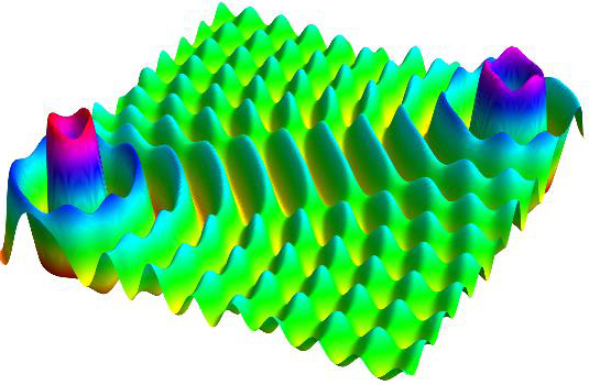
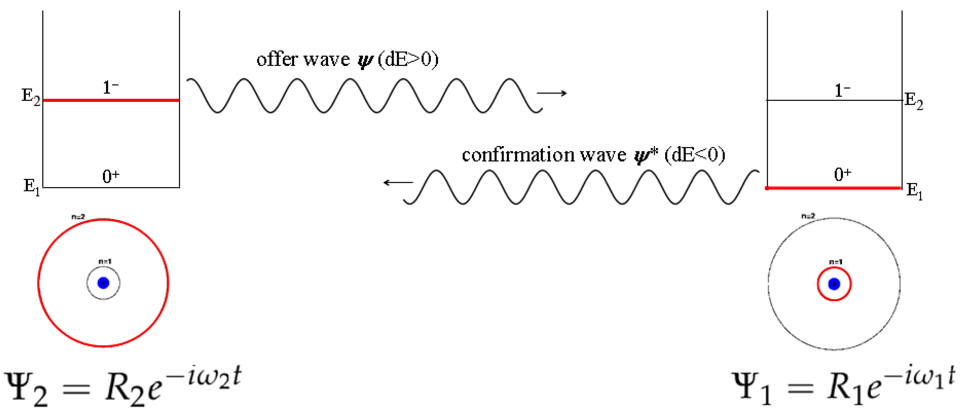
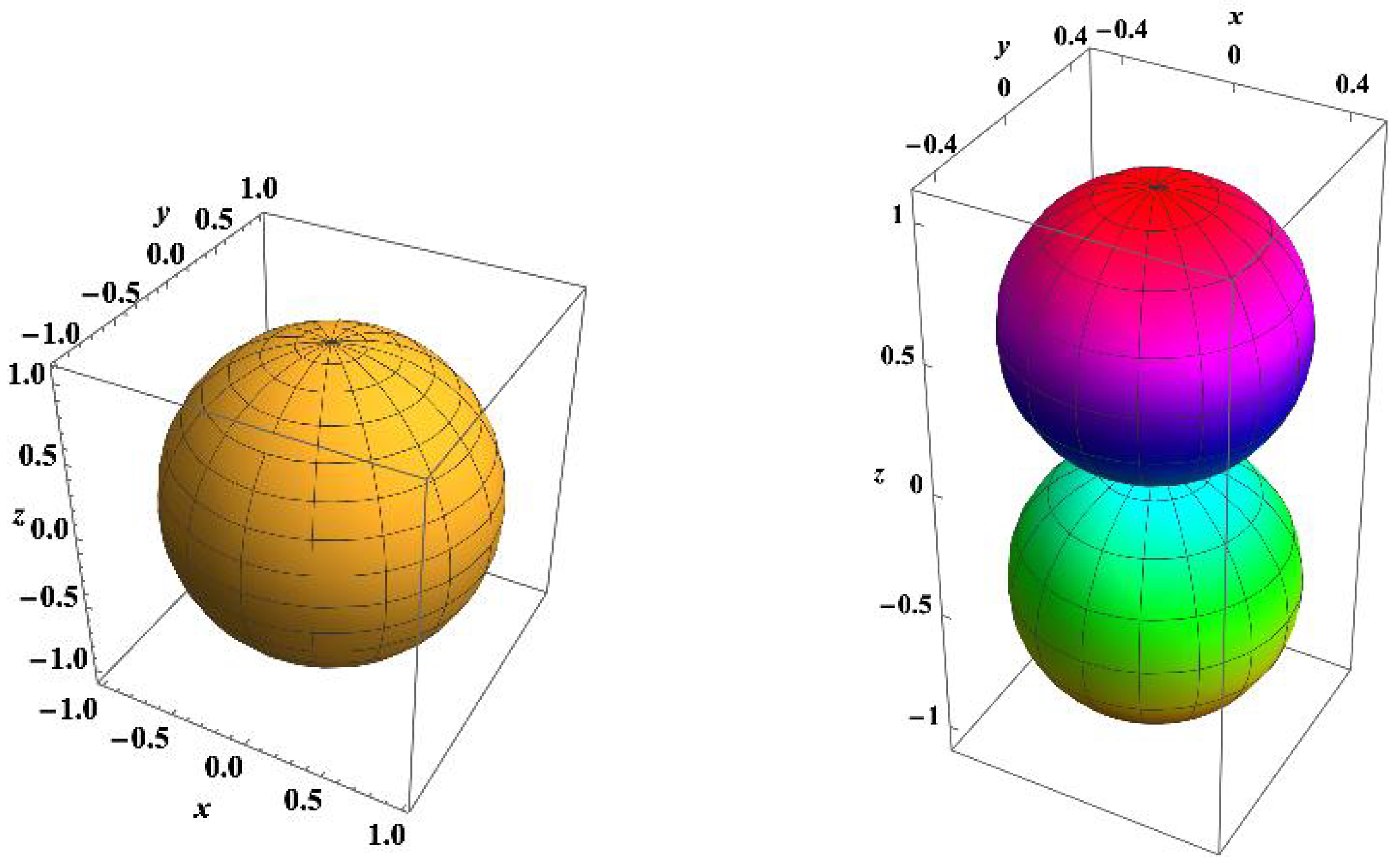
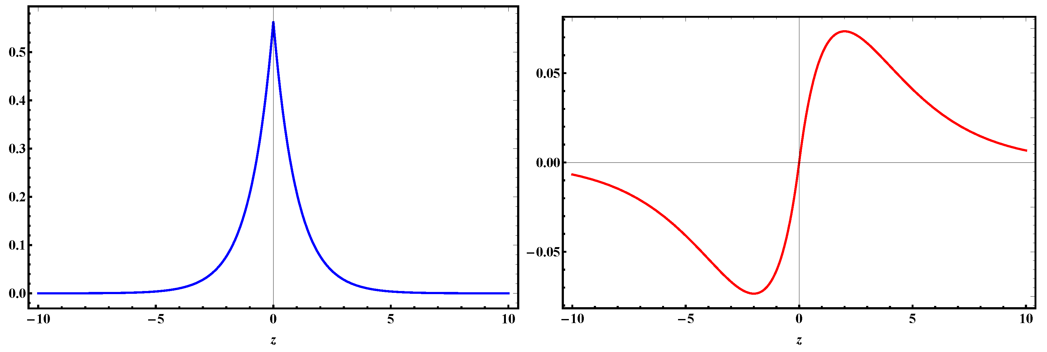
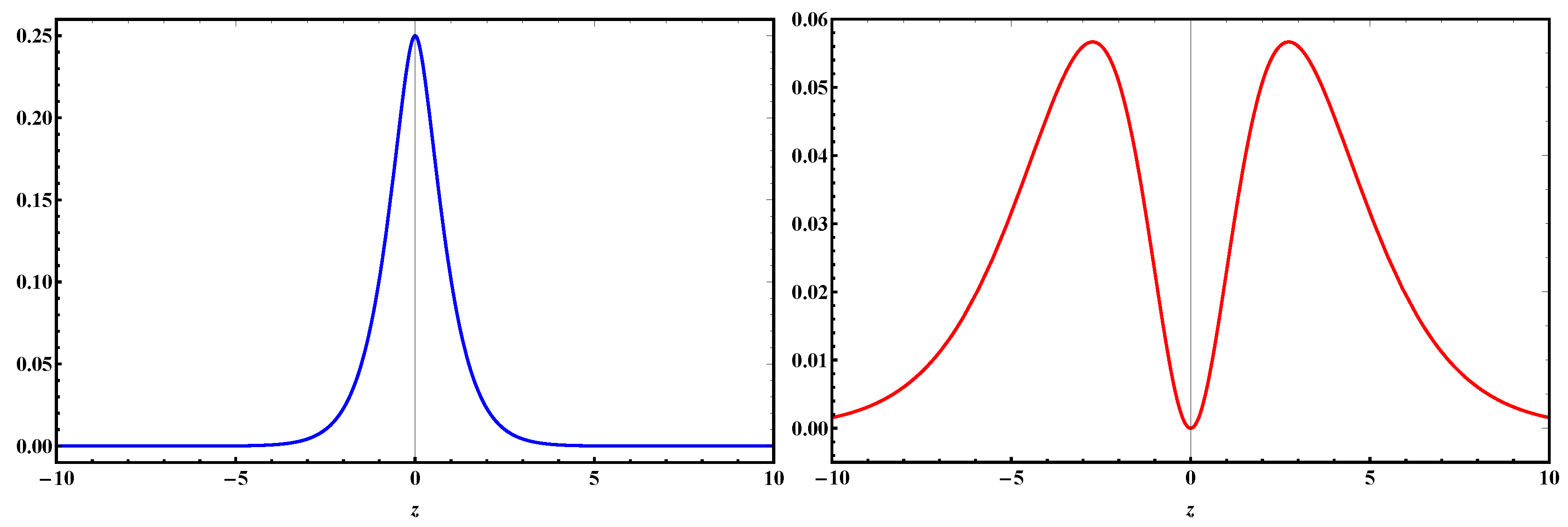
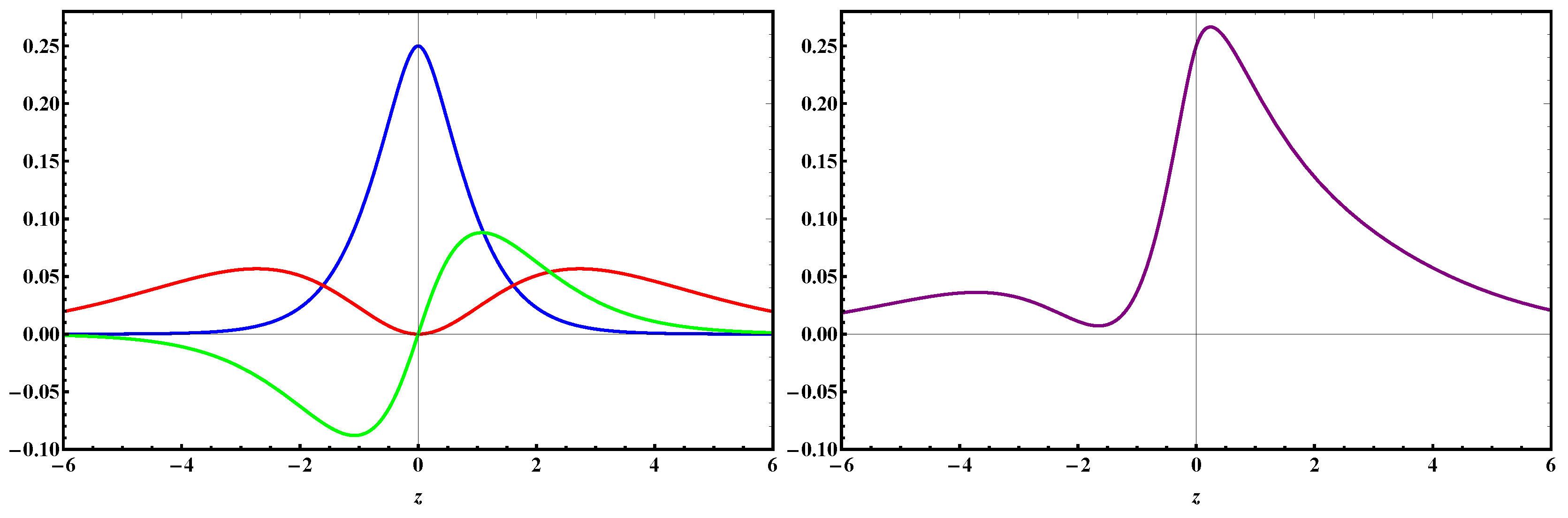
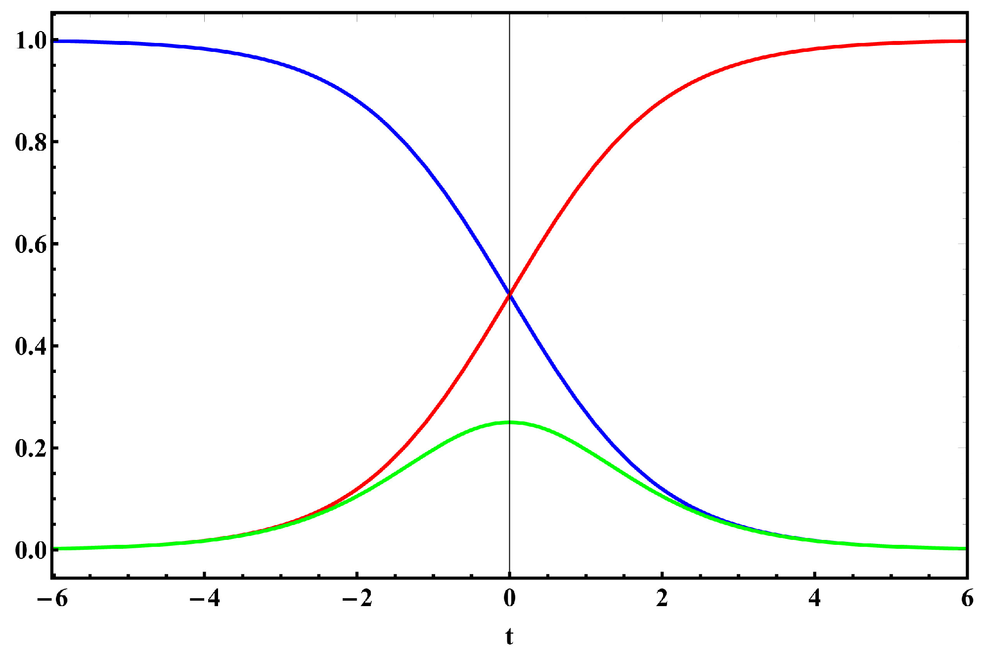
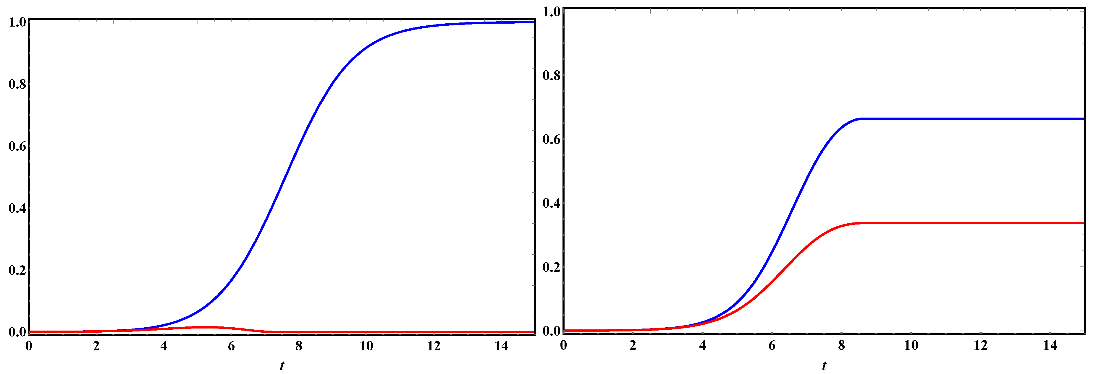
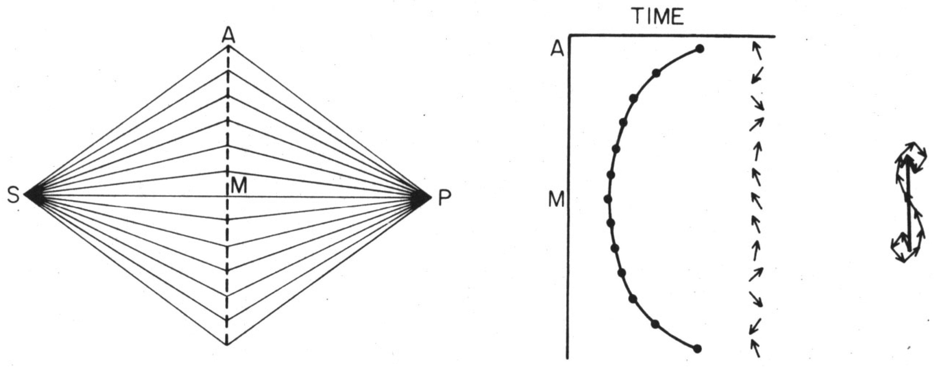
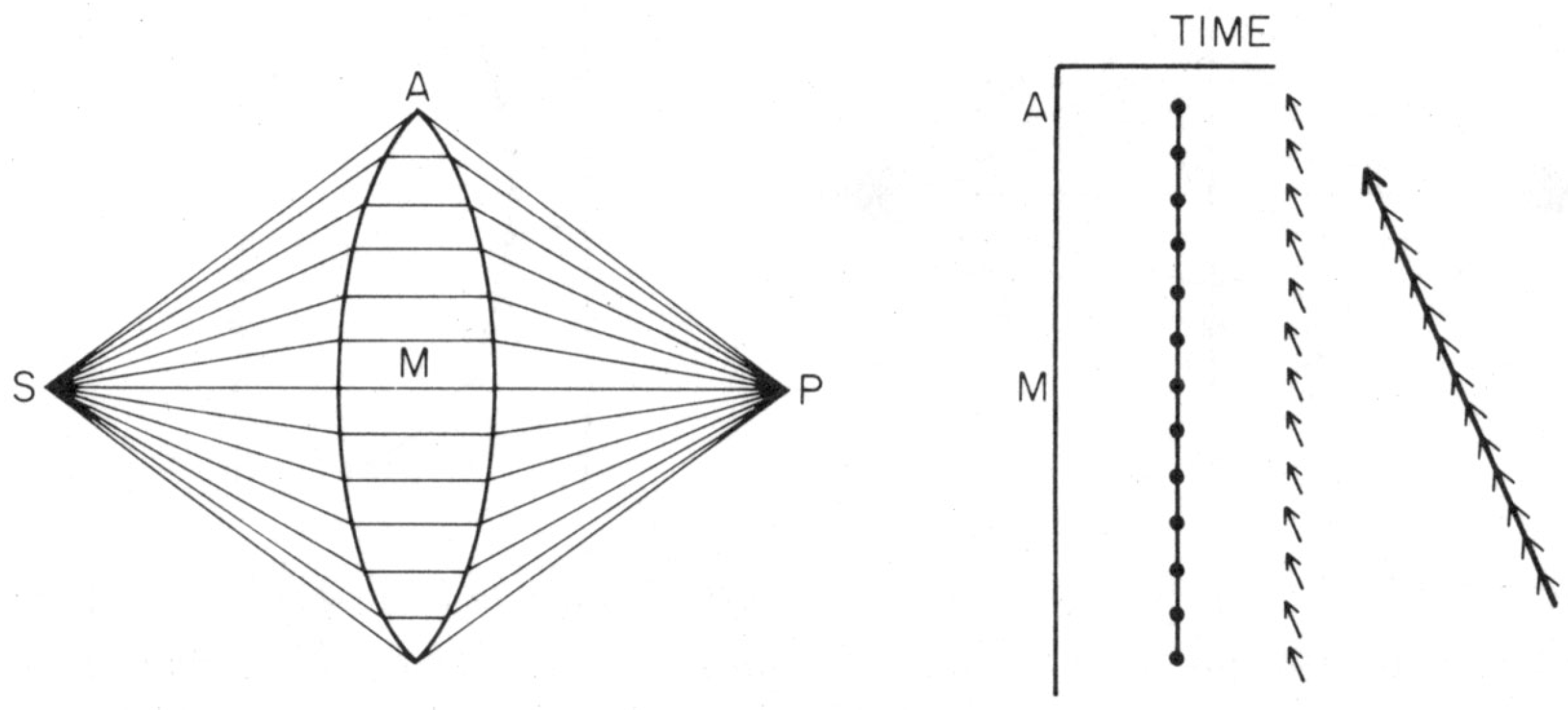
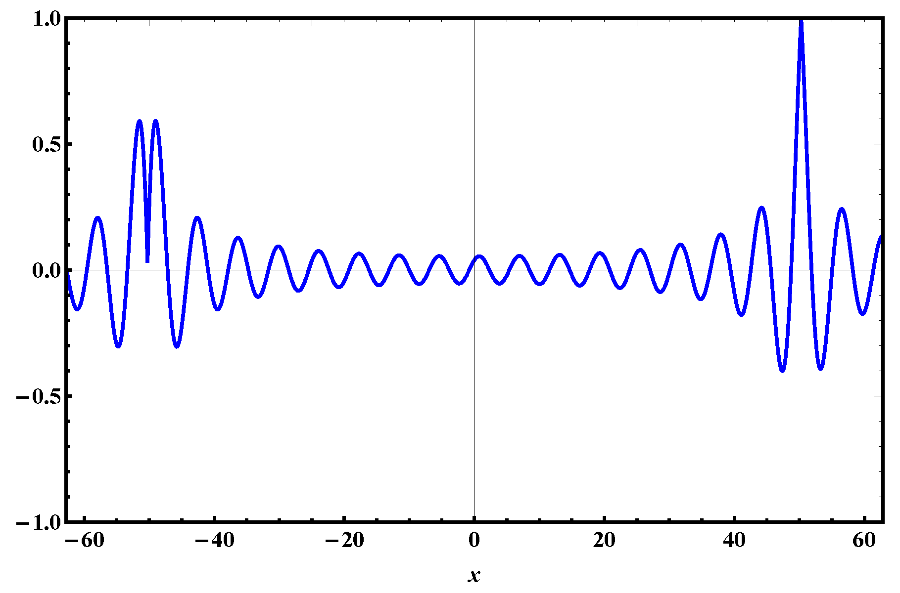
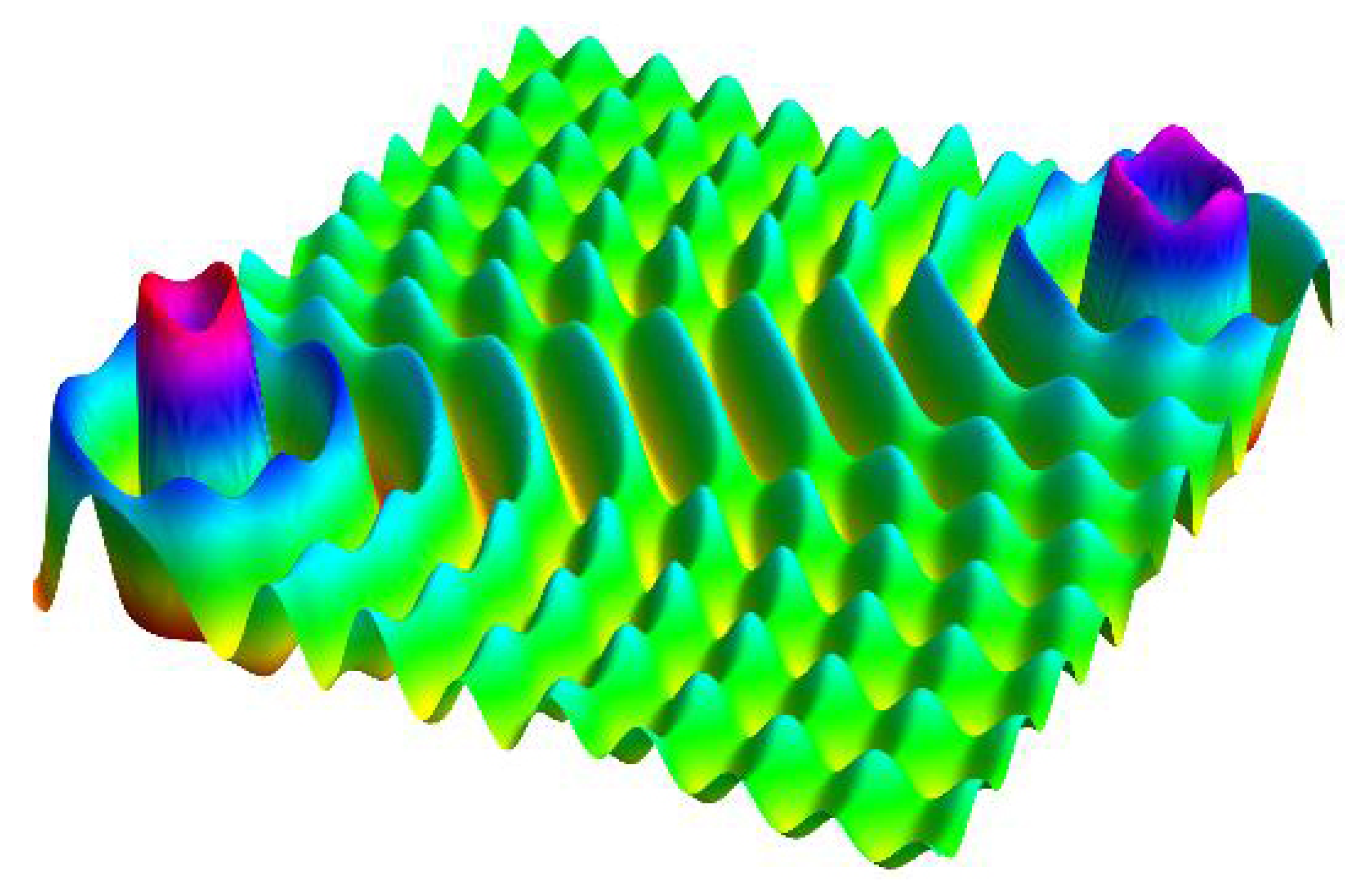
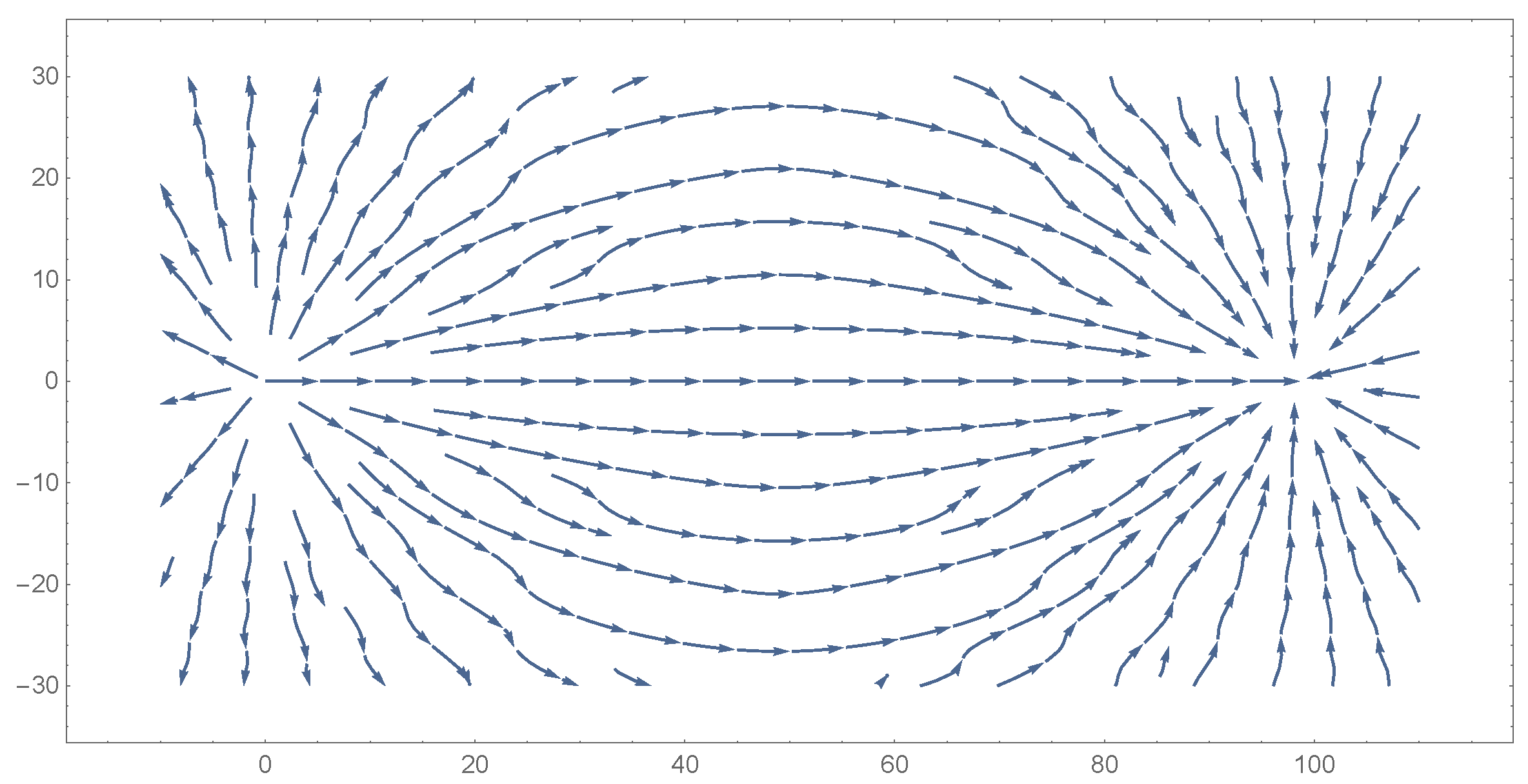
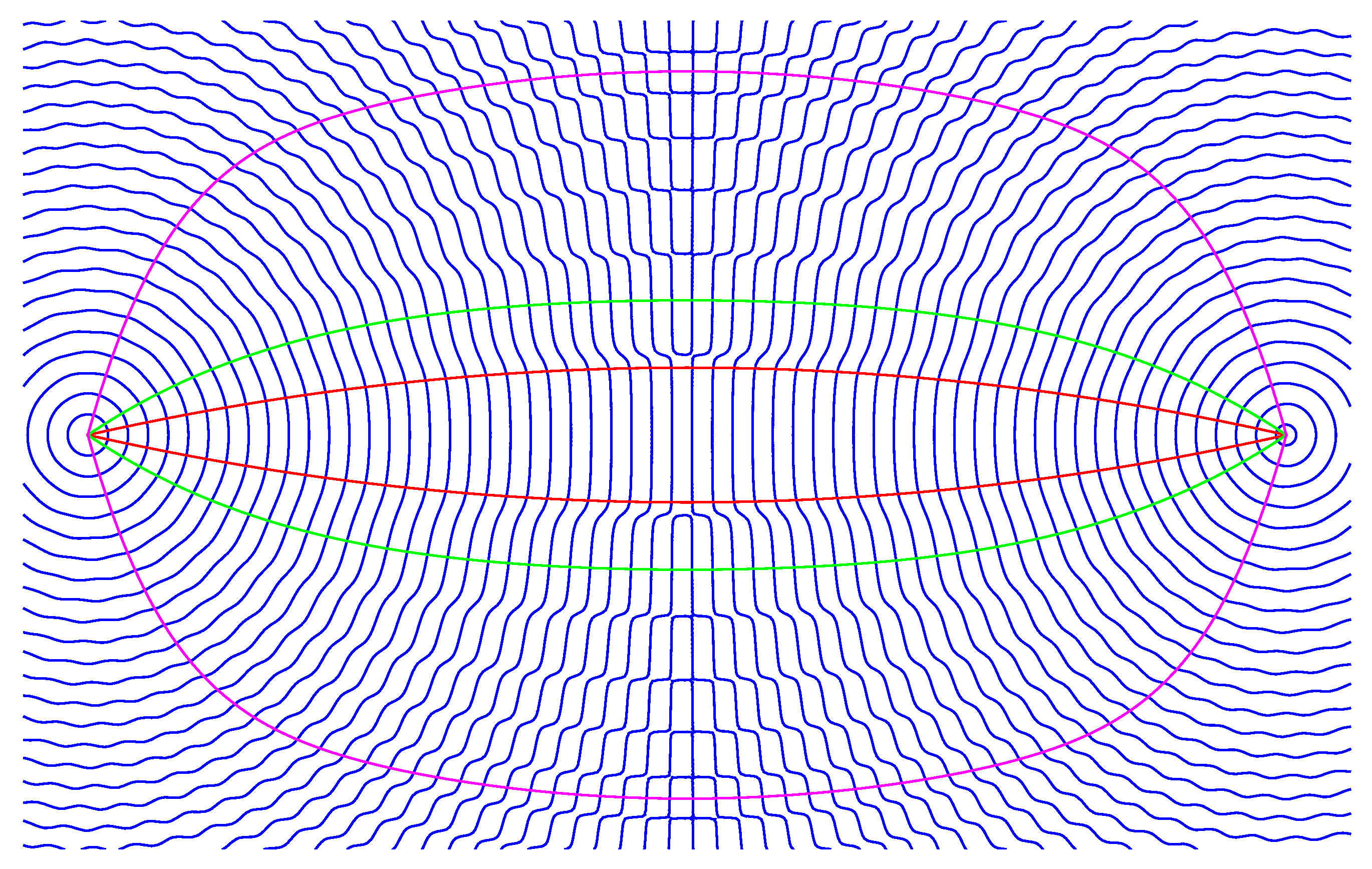
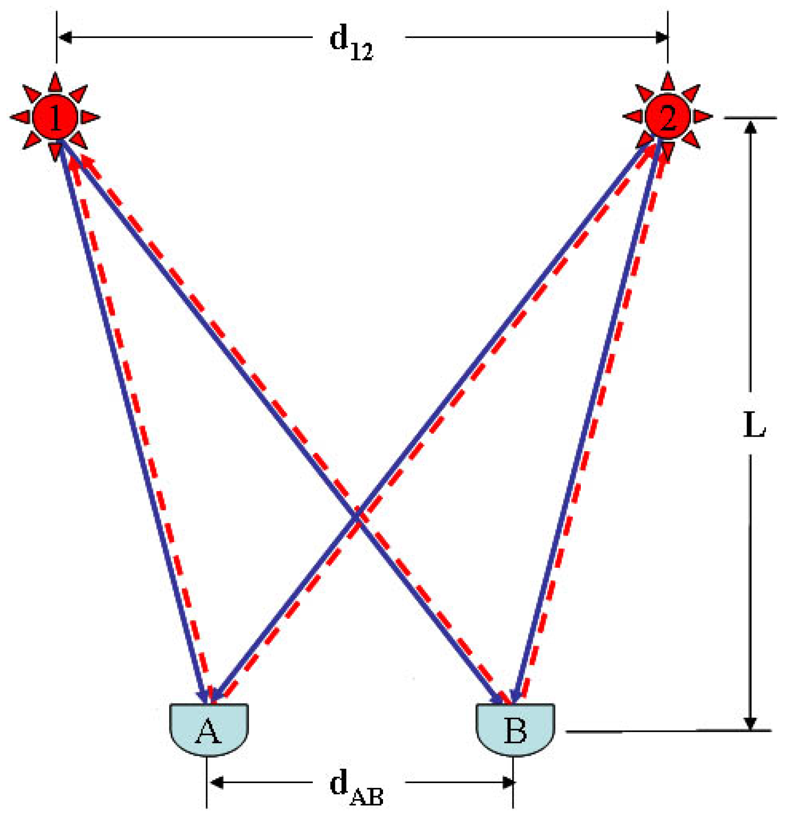
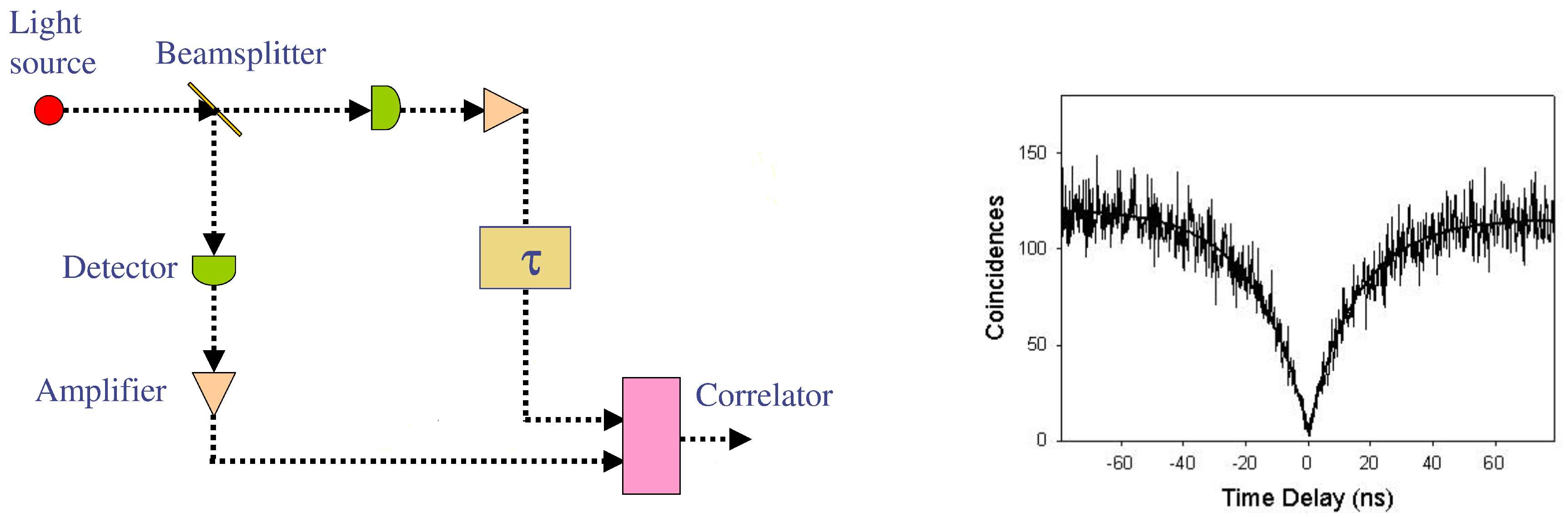
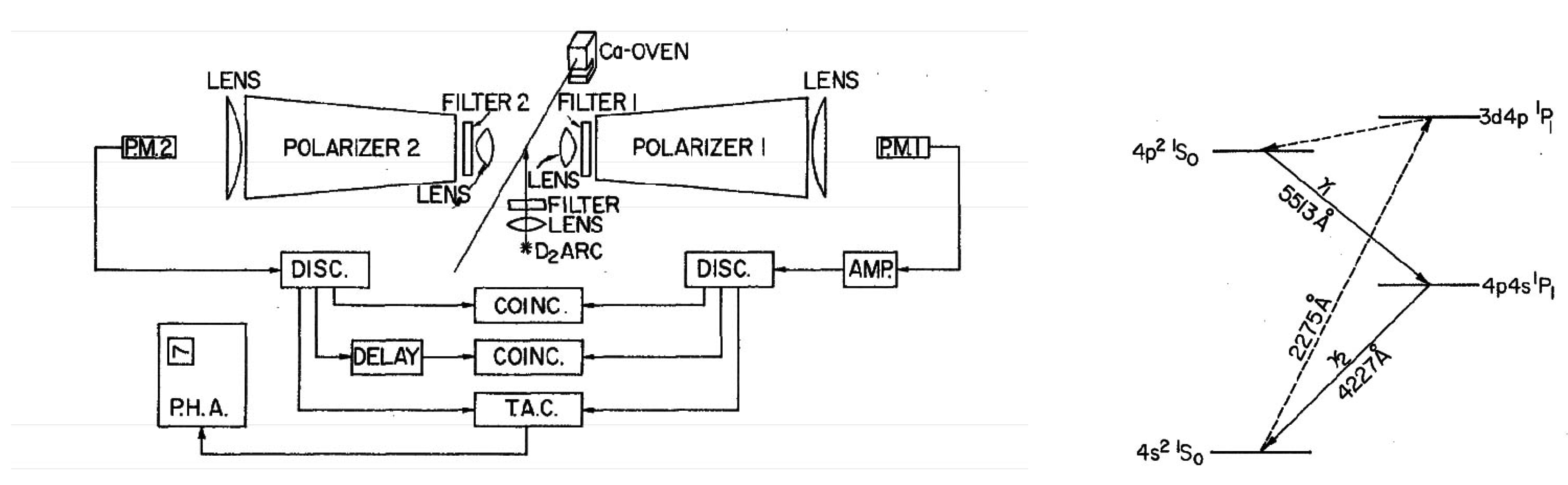
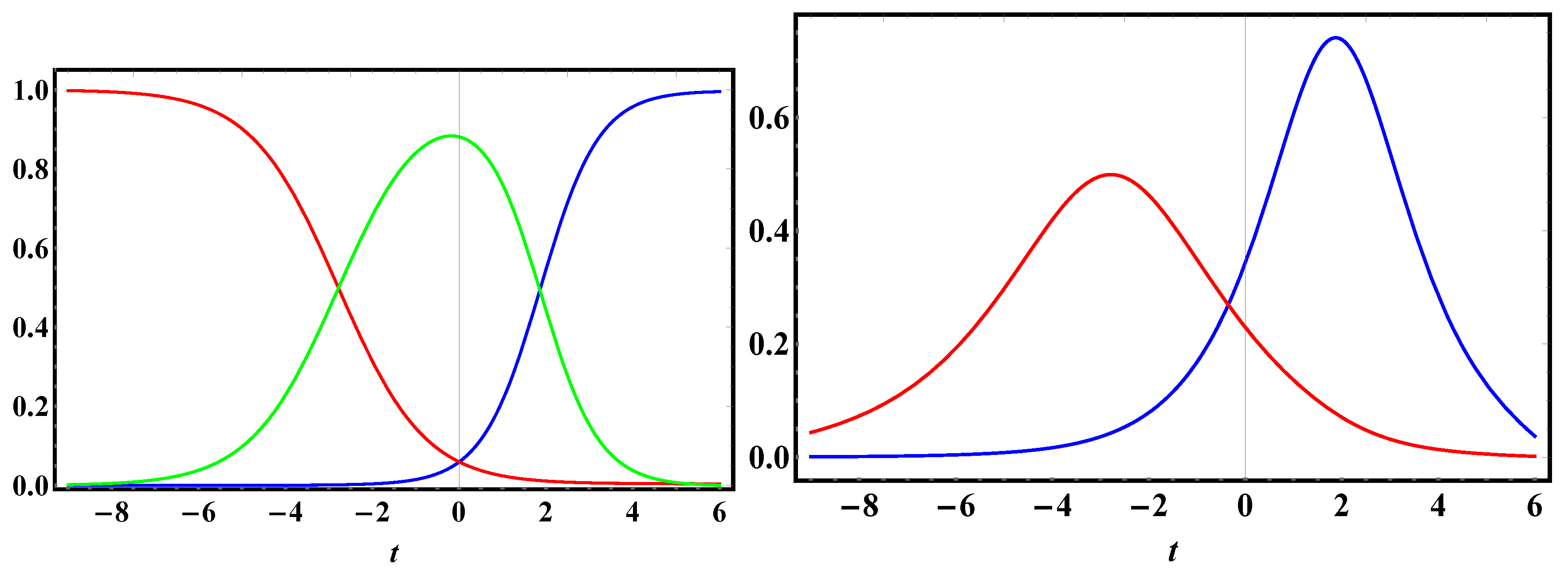
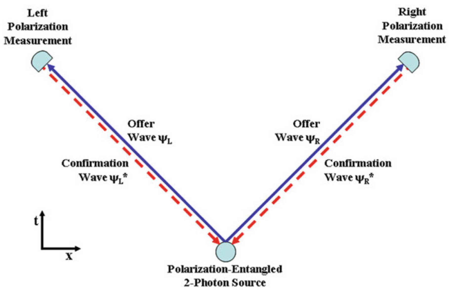
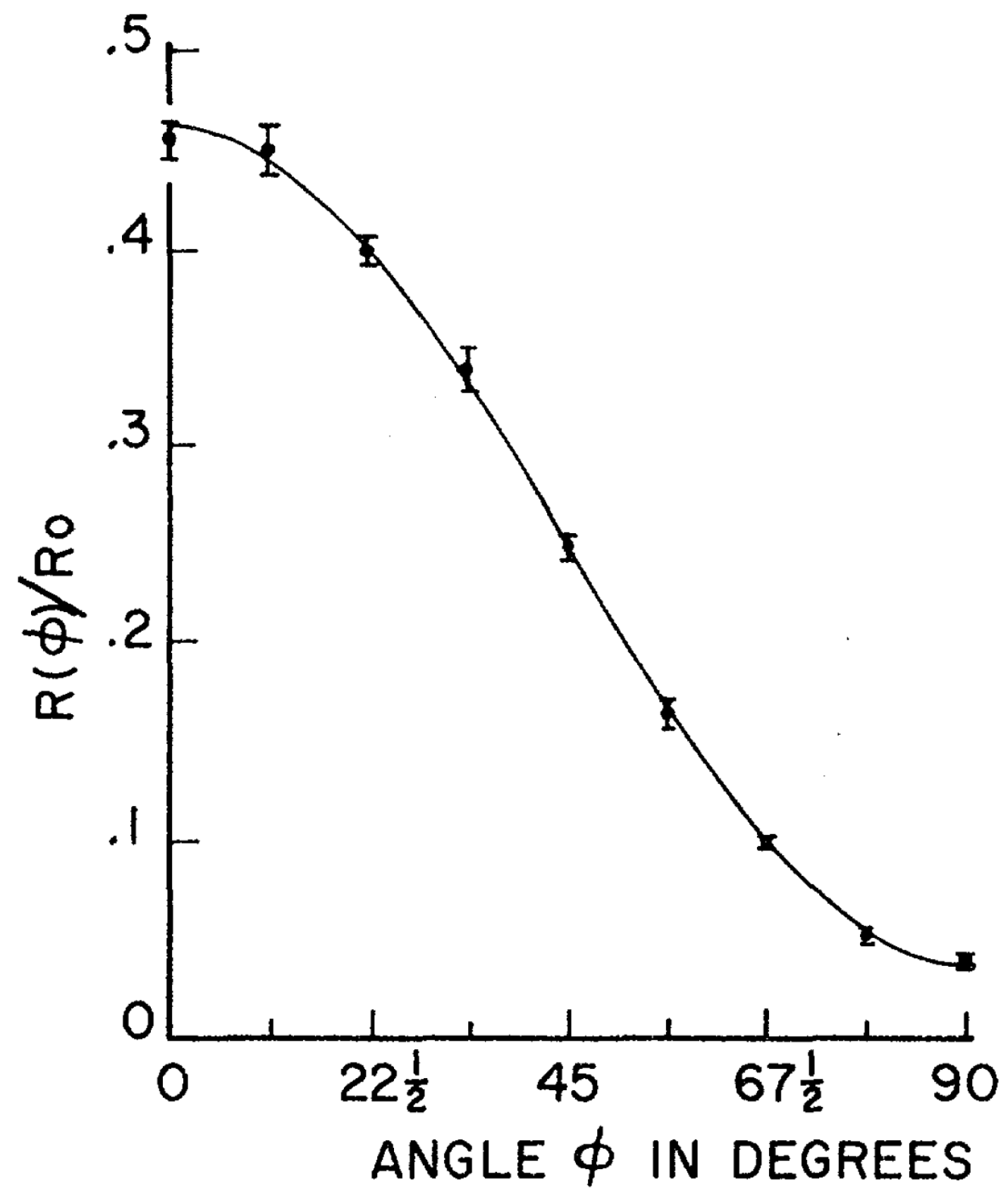