Article

Environmental Governance Cost Prediction of Transportation Industry by Considering the Technological Constraints

1
School of Business Administration, Zhejiang University of Finance & Economics, Hangzhou 310018, China
2
Decision Sciences Institute, Fuzhou University, Fuzhou 350108, China
*
Author to whom correspondence should be addressed.
Symmetry 2020, 12(8), 1352; https://doi.org/10.3390/sym12081352
Submission received: 25 July 2020 / Revised: 9 August 2020 / Accepted: 11 August 2020 / Published: 12 August 2020

Abstract

:
In order to solve the problem of environmental governance investment planning in the transportation industry, a cost prediction model is proposed under technological constraints, where the input output indictors emphasizes the flexibility of prediction and its characters are asymmetric, while the constructs of prediction model focuses on the standardization and its characters are symmetrical. The basic principle of the cost prediction model is based on an extended belief rule-based (EBRB) system to model the input-output relationship in investment planning, and a parameter learning model to improve the accuracy of the EBRB system. Additionally, the technological innovation factors are also embedded in the cost prediction model to investigate the influence of technology-related outcomes on investment planning. Finally, based on the data of environmental governance in China’s transportation industry from 2003 to 2016, the cost of transportation industry environmental management in China’s thirty provinces from 2017 to 2033 is predicted under the constraints of technological innovation. Results show that: (1) the accuracy of the proposed cost prediction model is higher than some existing cost prediction methods; (2) the predicted environmental governance costs have a significant regional difference; (3) the upgrading of technological innovation is conducive to saving the future environmental governance costs of the transportation industry in some provinces. In addition to the above results, the present study provides model supports and policy references for government decision makers in transportation industry-related environmental cost planning.

1. Introduction

The transportation industry is one of the three major carbon emission industries in China [1]. With the development of economies, the pollution emissions of the transportation industry increased rapidly. Reducing the pollution emission of the transportation industry has become one of the important tasks for countries in the world to deal with global warming [2]. The energy consumption of the transportation industry is larger than other industries, which involving more human, material and financial cost investment, and it is also one of the important factors affecting low-carbon development [3]. Effective cost planning and prediction can avoid the blind cost investment in low-carbon development, make the resources be effectively allocated and promote the sustainable development of the transportation industry [4].
Environmental governance cost refers to the cost of manpower, assets and energy invested by the government and enterprises in the process of environmental pollution discharge and control. The cost of environmental governance used in this paper is determined according to the principle of indicator selection in previous studies, in which labor, capital and energy consumption are common input costs of environmental pollution control. The environmental governance cost prediction of the transportation industry is the focus of low-carbon development. Existing studies on environmental cost mainly focus on the relationship between management cost and carbon emissions, such as the input-output performance analysis of carbon emissions based on data envelopment analysis (DEA) [5], the cost saving effect of carbon emission trading mechanism [3] and the environmental cost difference under different emission reduction measures [6]. In these studies, many scholars believed that the improvement of the existing environmental governance cost input mechanism is an important way to reduce carbon emissions [7,8,9]. Previous studies have also proposed different environmental cost calculation methods. For example, Yang et al. [7] predicted the cost of carbon compensation according to the carbon deficit theory, and also proposed the concept of social carbon cost to calculate the loss value of excessive carbon emissions on economic costs. In addition, there are some studies to measure environmental costs by exploring carbon prices, which are mainly based on the analysis of China′s carbon trading market mechanism [10]. However, few studies focused on environmental governance cost prediction of a specific industry. In other words, for the environmental governance cost prediction in the transportation industry, there is no effective method to investigate and predict the environmental governance cost in domestic research.
From the model construction of environmental cost prediction, the existing environmental governance cost prediction mainly focused on the impact of pollution emissions on economic cost loss, and the relevant methods are mainly linear regression analysis or theoretical analysis. For example, Lin et al. [11] used the generalized moment system estimation method of simultaneous equations to investigate the relationship between China′s urbanization, carbon emissions and economic growth, so as to evaluate the cost of carbon emissions, and analyze the future carbon emission strategies. The existing cost prediction methods mainly focus on the consideration of the overall environmental governance cost, such as the grey system model (GM (1.1)) [4], the adaptive neural fuzzy inference system (ANFIS) [12], etc. Therefore, it can be found that the current researches on environmental governance cost prediction methods have the following limitations: (1) the studies on environmental governance cost were mainly based on strategy or goal orientation, and the relevant prediction methods failed to obtain the environmental governance cost prediction value of the transportation industry in the future; (2) although the existing studies have carried out a certain correlation analysis on the relationship between environmental management and technological innovation, the construction of environmental governance cost prediction model under technical constraints has not yet been realized; (3) the cost prediction methods were mainly based on the field of environmental governance [13], and rarely involved the future cost prediction of different industries.
Therefore, to overcome the limitations of the existing studies, this paper proposes an environmental governance cost prediction model based on an extended belief rule-based (EBRB) system and technological constraints, in which the EBRB system was proposed by Liu et al. [14] and has demonstrated its excellent prediction performance on many real problems [15]. According to the modeling mechanism of EBRB system, historical input-output data pairs can be used to efficiently generate an extended belief rule base, which is the rule base of the EBRB system, and the basic parameters in the rule base should be optimized to enhance the accuracy of the EBRB system [16]. Hence, a parameter learning method is proposed to optimize basic parameters by using historical input-output data pairs for better cost prediction. Moreover, the technological innovation is an important factor in the environmental governance cost prediction of the transportation industry, so the influence of technology-related outcomes on investment planning is regarded as a dependent variable to adjust the predicted costs by the proposed model for environmental governance cost prediction of the transportation industry.
To validate the effectiveness of the proposed model, the data of China’s environmental statistical yearbook, China′s energy statistical yearbook, and China’s statistical yearbook from 2004 to 2017 are selected as historical data to build a cost prediction model for predicting the costs of the transportation industry related to 30 provinces in the mainland of China (except Taiwan and Tibet), in which the environmental governance inputs and outputs of the transportation industry for each province from 2003 to 2016 are taken as training data. Additionally, based on the policy objectives of the 13th five year plan and the technological innovation differences among different provinces, the environmental governance costs of the transportation industry in China from 2017 to 2033 are regarded as the targets to be predicted using the proposed model. In the comparison of existing methods, some commonly used cost prediction methods are introduced to compare accuracy with the proposed model and its effectiveness is also verified by considering the constraints of technological innovation in the transportation industry, which provides a certain reference for the government to make effective environmental cost budget.

2. A Review of Traditional EBRB System

The EBRB system was proposed by Liu et al. [14] and has been widely used in various prediction problems [15]. An EBRB system consists of a series of extended belief rules with embedding the belief structure into all attributes, where the kth rule (k = 1, …, L) can be expressed as:
R k : I F   U 1   i s   { ( A 1 , j , α 1 , j k ) ; j = 1 , , J 1 }   a n d a n d   U M   i s   { ( A M , j , α M , j k ) ; j = 1 , , J M } , T H E N   D   i s   { ( D n , β n k ) ; n = 1 , , N }
where α i , j k ( 0 α i , j k 1 ) and β n k ( 0 β n k 1 ) are the belief degrees of referential value Ai,j and consequent Dn in the kth rule; δ i ( 0 < δ i 1 ) and θ k ( 0 < θ k 1 ) are the weight of the ith antecedent attribute and the kth rule. Furthermore, the extended belief rules of an EBRB system are generated from a set of input-output data pairs without any iterative optimization algorithm, the specific steps in the case of having M input indicators Ui (i = 1, …, M) and one output indicator D for the cost prediction in the transportation industry can be expressed as follows:
Step 1: To initialize the basic parameters of an EBRB system. The basic parameters, including the utility value u(Ai,j) of all referential values, the utility value u(Dn) of all consequents Dn (n = 1, …, N), and the weight of all input attributes δ i (i = 1, …, M), should be determined by using the domain knowledge of experts.
Step 2: To calculate the belief degree of all indicators. Firstly, T training data <xk, yk> (k = 1, …, T) are used to generate extended belief rules, where xk = (xk,1, …, xk,M) denotes the input vector of the kth training data, xk,i represents the input data corresponding to the ith input indicator in the kth input indicator vector, and yk represents the kth output data. On the basis of the utility-based transformation method, these T input-output data pairs can be transformed into the belief degree of input and output indicators in an extended belief rule. The calculation formula of belief degree in the ith input indicator is as:
S ( x k , i ) = { ( A i , j , α i , j k ) ; j = 1 , , J i }
where
α i , j k = u ( A i , j + 1 ) x k , i u ( A i , j + 1 ) u ( A i , j )   a n d   α i , j + 1 k = 1 α i , j k ,   i f   u ( A i , j ) x k , i u ( A i , j + 1 )
α i , t k = 0 ,   f o r   t = 1 , , J i   a n d   t j , j + 1
Similarly, the belief degree of output indicator can be calculated as follows:
S ( y k ) = { ( D n , β n k ) ; n = 1 , , N }
Step 3: To calculate the rule weights of the EBRB system. Firstly, according to the belief degrees of input and output indicators obtained from Step 2, the similarity of rule antecedent (SRA) and consequent (SRC) are calculated as follows:
S R A ( R l , R k ) = 1 max t = 1 , , M { j = 1 J t ( α t , j l α t , j k ) 2 2 } ; l = 1 , , L ; l k
S R C ( R l , R k ) = 1 n = 1 N ( β n l β n k ) 2 2 ; l = 1 , , L ; l k
Next, the inconsistency of the kth rule can be obtained by:
I D ( R k ) = l = 1 , l k L ( 1 exp { ( S R A ( R l , R k ) S R C ( R l , R k ) 1 ) 2 ( 1 S R A ( R l , R k ) ) 2 } )
Finally, the weight of the kth rule is calculated by:
θ k = 1 I D ( R k ) j = 1 L I D ( R j )

3. Environmental Governance Cost Prediction by EBRB System for the Transportation Industry

In order to improve the performance of the ERBB system in the cost prediction in the transportation industry, parameter learning is introduced to optimize the basic parameters of the EBRB system in Section 3.1, and the technology constraint is considered to adjust the EBRB system in Section 3.2.

3.1. Parameter Learning to Optimize Basic Parameters of EBRB System

In the generation of traditional EBRB system in Section 2, the values of basic parameters are usually given by experts, which have a certain subjectivity, and are therefore impossible to ensure the high accuracy of the EBRB system. Therefore, a parameter learning model is introduced to improve the EBRB system. Considering that the basic parameters in the EBRB system include indicator weights, utility values of referential values for all input indicators and consequents for consequent attribute, the corresponding constraints can be defined as follows:
(1)
For the indicator weight of the ith input indicator, the constraint conditions are as follows:
0 < δ i 1 ; i = 1 , , M
(2)
For the utility values of the ith input indicator, the constraint conditions are as follows:
u ( A i , j ) u ( A i , j + 1 ) ; i = 1 , , M ; j = 1 , , J i 1
u ( A i , 1 ) = l b i ; i = 1 , , M
u ( A i , J i ) = u b i ; i = 1 , , M
where lbi and ubi is the lower and upper bounds of ith input indicator.
(3)
For the utility values of the output indicator, the constraint conditions are as follows:
u ( D n ) u ( D n + 1 ) ; n = 1 , , N 1
u ( D 1 ) = l b
u ( D N ) = u b
where lb and ub is the lower and upper bounds of output indicator.
For the objective function of parameter learning of EBRB system, suppose that there are T input-output data <xt, yt> (t = 1, …, T) and the inference result of the EBRB system for each data is f ( x t ) , the objective function is defined as follows:
  min   M A E ( { δ i , u ( A i , j ) , u ( D n ) } ) = t = 1 T | y t f ( x t ) |
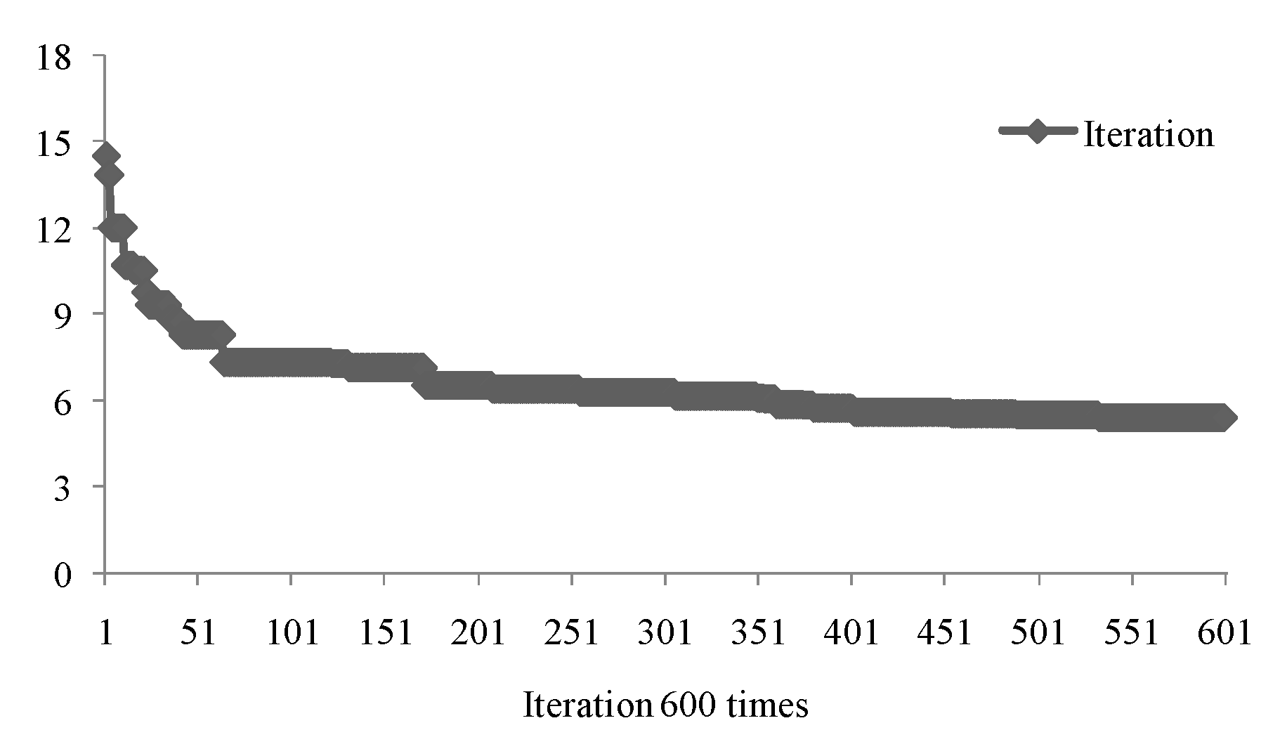
In order to obtain the minimum values of the objective function shown in Equation (17) under the constraints shown in Equations (10) to (16), a differential evolution (DE) algorithm in further introduced and the detailed processes are as follows:
Suppose that the basic parameters in the EBRB system are optimized through C individuals and S iterations in the DE algorithm, in which the basic parameters in the cth individual and the sth iteration can be expressed as:
P s , c = { p k s , c ; k = 1 , , K } = { δ i s , c , u ( A i , j ) s , c , u ( D n ) s , c } ; s = 1 , , S ; c = 1 , , C
where δ i s , c denotes the indicator weights of i (i = 1, …, M) input indicator; u ( A i , j ) s , c is the utility value of Ai,j; u ( D n ) s , c is the utility value of Dn; p k s , c denotes the kth basic parameter; K denotes the total number of basic parameters. When ubk and lbk are the upper and lower bounds of kth parameter p k s , c , the initial values of basic parameters can be obtained:
p k 0 , c = l b k + ( u b k l b k ) × r a n d o m   ( 0 , 1 ) ; c = 1 , , C ; k = 1 , , K
Next, in the sth iteration, for any individual P s , c , three different individuals P s , c 1 , P s , c 2 and P s , c 3 are randomly selected from C individuals, and then a new individual P s , c 0 is generated:
p k s , c 0 = { p k s , c , i f   r a n d o m   ( 0 , 1 ) > C R p k s , c 1 + F × ( p k s , c 2 p k s , c 3 ) , o t h e r w i s e ; c = 1 , , C ; k = 1 , , K
where F is the cross factor, CR is the variation factor.
Then, in the sth iteration, when the parameter value of P s , c 0 exceeds the constraint conditions, the value is re assigned according to Equation (19). The value of the objective function shown in Formula (17) is calculated by the parameter value P s , c 0 , and finally P s , c is updated by:
P s , c = { P s , c 0 ,   i f   M A E ( P s , c 0 ) < M A E ( P s , c )   P s , c ,   o t h e r w i s e
Finally, when the total number of iterations is equal to the given number of iterations, the minimum objective function value is taken as the optimal value and the corresponding basic parameters as the optimal parameters of EBRB system.

3.2. Cost Prediction Using the Improved EBRB System with Technological Constraints

After obtaining the EBRB system improved by the parameter learning model, technological constraints are considered to improve the rule inference process of EBRB system, which is used to produce an output for replying any given input data. Based on the original rule inference of EBRB system in 14, the rule inference process under technological constraints has the following steps:
Step 1: To calculate technological innovation factors for the EBRB system. Suppose that P technological innovation indicators are used to calculate technological innovation factors and their historical data are zk,p (k = 1, …, T; p = 1, …, P). Due to the incommensurability among these P indicators, the historical data of these indicators need to be normalized to eliminate dimensional units using
z ¯ k , p = { z k , p min i = 1 , T { x k , i } max i = 1 , S { z k , i } min i = 1 , S { z k , i } , z k , p Ω P o s i t i v e max i = 1 , S { z k , i } z k , p max i = 1 , S { z k , i } min i = 1 , S { z k , i } , z k , p Ω N e g a t i v e
where z ¯ k , p is the normalized value of the pth (p = 1, …, P) indicator in the kth (k = 1, …, T) data; z k , p Ω P o s i t i v e denotes that zk,p is the positive value which is larger the better; z k , p Ω N e g a t i v e denotes that zk,p is the negative value which is larger the better.
Afterwards, the normalized values are used to calculate the technological innovation factors of the kth data, denoted as TIFk, by:
T I F k = p = 1 P z ¯ k , p
Step 2: To consider technological constraint in the EBRB system. When the technological innovation factors TIFk (k = 1, …, T) are considered in the EBRB system, an extended dataset can be generated by combining the original data <xk, yk> (k = 1, …, T) and the technological innovation factors TIFk, namely <xk, TIFk, yk>. On the basis of the new dataset and taking the technological innovation factor as a new input indicator of the EBRB system, an EBRB system with the consideration of technological constraint can be generated, according to Section 2 and Section 3.1.
Step 3: To calculate the activation weight of each rule. Suppose that a new input data vector including technological innovation factor, denotes as x = (xi; i = 1, …, M + 1), is provided for the EBRB system, and the input data can be transformed into belief distribution S ( x i ) = { ( A i , j , α i , j ) ; j = 1 , , J i } using Equations (3) and (4). Afterwards, the activation of the kth (k = 1, …, L) rule can be calculated as follows:
w k = θ k i = 1 M + 1 ( S k ( x i , U i ) ) δ i l = 1 L ( θ l i = 1 M + 1 ( S l ( x i , U i ) ) δ i ) ,   δ i = δ i max i = 1 , , M + 1 { δ i }
where δ i is the weight of the ith indicator; θ k is the weight of the kth rule; S k ( x i , U i ) denotes the individual matching degree of input indicator for the kth rule and it can be calculated as follows:
S k ( x i , U i ) = 1 d k ( x i , U i ) = 1 j = 1 J i ( α i , j α i , j k ) 2 2
where α i , j k ( j = 1 , , J i ) is the belief degree of the kth rule in referential value Ai,j; d k ( x i , U i ) denotes the distance between input data and rule, then the active weight can be calculated:
Step 4: To integrate all activated rules based on the evidence reasoning (ER) algorithm. According to the analytical ER algorithm, the rule which has activation weight wk > 0 should be integrated by:
β n = k = l L ( w k β n k + 1 w k i = 1 N β i k ) k = l L ( 1 w k j = 1 N β j k ) i = 1 N k = l L ( w k β i k + 1 w k j = 1 N β j k ) ( N 1 ) k = l L ( 1 w k j = 1 N β j k ) k = l L ( 1 w k )
Next, when the utility values for N consequents of output indicators are {u(Dn); n = 1, …, N}, the predicted cost for the environmental governance in the transportation industry can be obtained by:
f ( x ) = i = 1 N ( u ( D i ) β i ) + u ( D 1 ) + u ( D N ) 2 ( 1 i = 1 N β i )
For the above-mentioned cost prediction process using the EBRB system, it is worth noting that, when future input data are provided, the EBRB system is also able to predict the future costs used for environmental governance in the transportation industry. The detailed steps are as follows:
Step 1: To calculate the future input data of the EBRB system. Suppose that the input indicators of the EBRB system can be divided into two categories: positive and negative. The positive indicators are those indictors for maximization, such as benefit, whose values are always the larger the better. The negative indicators are those for minimization, such as cost, whose values are better when smaller. The values of the rth positive (r = 1, …, M1) attribute and the fth (f = 1, …, M2) negative attribute are denoted as x ^ r ( t ) and x ^ f ( t ) in the future the tth (t = 0, …, ) year. Additionally, suppose that ar is the target change ratio of the rth positive indicator and bf is the target change proportion of the fth negative indicator of the transportation industry in the future. Hence, the calculation of the future input data of the EBRB system can be obtained as follows:
x ^ r ( t ) = { x r ;   i f   t = 0 ( 1 + a r ) x ^ r ( t 1 ) ;   o t h e r w i s e ;   r = 1 , , M 1
x ^ f ( t ) = { x f ;   i f   t = 0 ( 1 b f ) x ^ f ( t 1 ) ;   o t h e r w i s e ;   f = 1 , , M 2
Step 2: Future cost prediction with technological constraints. According to the future input data x ^ r ( t ) and x ^ f ( t ) of the transportation industry, the predicted environmental governance costs in the transportation industry can be obtained according to Equations (24) to (27).

4. Case Study of Cost Prediction in the Transportation Industry

In this section, the proposed model shown in Section 3 is used to predict the environmental governance cost of China′s transportation industry, in which the data resource and variable determination are introduced in Section 4.1, the model development and results discussion are provided in Section 4.2 and future environmental governance cost prediction with technology constraint is shown in Section 4.3.

4.1. Data Resource and Variable Determination

The cost prediction for the transportation industry is mainly based on environmental input and output historical data of 30 provinces in mainland China (except Tibet and Taiwan) from 2004 to 2017. These historical data are derived from the China Environmental Statistical Yearbook, the China Energy Statistical Yearbook and the China Statistical Yearbook. In order to ensure that the input and output indicators of the transportation industry are consistent with existing studies, the input-output indicators applied in the previous studies are shown in Table 1. Thus, in this study, the industrial added value (IAV) of the transportation industry and the carbon dioxide (CO2) emissions of the transportation industry are taken as input indicators, and the labor input, capital investment and energy consumption of the transportation industry are taken as output indicators. The statistical analysis of specific input and output indicators is shown in Table 2.
The labor and capital input has highly related to the increase of IAV in transportation development, and the transportation industry is one of the three major CO2 emission industries in China, so taking carbon dioxide as an input indicator can better fit the actual environmental governance process of the transportation industry. In this paper, cost prediction is the goal of this study, so in the model construction, labor, capital and other indicators related to cost are taken as the output indicators of the prediction model, while pollution emissions and industrial added value are taken as input indicators.
In addition to the input and output indicators in Table 2, technological innovation is also a key factor that can affect the environmental governance cost of the transportation industry. Therefore, technological innovation factor (TIF) is regarded as one of input indicators in the cost prediction model, in which the indicators related to TIF and their specific representation are summarized in Table 3.
According to the 13th five year development plan put forward by the Chinese government in 2016, GDP should grow at the rate of 6.5% per year, and the carbon dioxide emission should decrease at the rate of 2.085%. Assuming that the level of technological innovation increases by 5% per year, the target input value of environmental governance cost of China′s transportation industry from 2017 to 2033 can be obtained. The specific statistics are shown in Table 4.

4.2. Model Development and Results Discussion of Cost Prediction with Technological Constraint

In this section, the application of the proposed model is introduced to specifically show the process of predicting the environmental governance cost in the transportation industry. Without of loss generality, the prediction of Beijing’s energy consumption from 2016 to 2033 is taken as an example when considering technological constrains.
Firstly, according to Section 3.2, a technological innovation factor should be calculated based on the technological innovation indicators shown in Table 3, because of considering the technological innovation factor in the cost prediction models. Adding to the data of input and output indicators shown in Table 2, the initial value of the basic parameters used to generate an EBRB system can be determined by equally splitting the range of lower and upper bounds in each indicator when the number of utility values in input and output indicators are assumed to be five, namely very low (VL), low (L), medium (M), high (H) and very high (VH). The details of these initial values of the basic parameters are shown in Table 5.
According to the parameter learning shown in Section 3.1, the optimized values of the basic parameters can be obtained when setting 600 iterations for the DE algorithm. The specific iterative process is shown in Figure 1. It is clear from Figure 1 that the iterative results tend to converge and the error between the predicted cost and the actual cost is minimized after 600 iterations. The optimized values of the basic parameters are shown in Table 5. It can be seen from Table 5 that the weight of IAV is the largest, which is 0.8318, followed by the weight of CO2, which is 0.8220. The weight of TIF is lower than that of IAV and CO2, which is 0.7787. From the view of the utility values of input and output indicators, the utility values of all indicators have certain changes compared with the initial value shown in Table 4. For example, the initial utility values of IAV are {u(VL) = 310, u(L) = 478, u(M) = 647, u(H) = 815, u(VH) = 983} in Table 5 and the optimized utility value of IAV are {u(VL) = 310, u(L) = 529, u(M) = 714, u(H) = 814, u(VH) = 983} in Table 6.
Based on the optimal values of basic parameters, the belief distributions and rule weights of the EBRB system can be generated from environmental input and output historical data according to Section 2, and the predicted environmental governance cost of each province can be obtained according to Section 3.2. Figure 2 shows the fitting degree and prediction error between the predicted costs and the actual costs. It is obvious that the predicted values fit well with the actual value from 2004 to 2017. The prediction error of most provinces is less than 10 and the cost prediction error in 2014 is about 30, which is actually only 2.9% of the actual value, according to the actual energy consumption of Beijing in 2014 to 2017.
Based on the above-mentioned of model development for a cost prediction model, the environmental governance costs of 30 provinces in China can be accurately predicted as well, using the input and output data of transportation environmental governance of 30 provinces in the mainland of China from 2003 to 2016. According to Figure 3, Figure 4 and Figure 5, it can be found that the compared results between actual cost and predicted cost in different regions show a high fitness, and the prediction error is lower in labor and energy prediction compared to capital prediction, but most regions’ cost prediction have shown high accuracy.
In order to effectively verify the accuracy of the proposed model, the accuracy of the proposed cost prediction model is compared, with two existing cost prediction models, namely GM (1.1) and ANFIS. The effectiveness of different cost prediction models is measured by the following criteria: (1) average absolute error (MAE); (2) average absolute percentage error (MAPE). The specific comparison results are shown in Table 7, when using the environmental input and output historical data of 2017 as testing data. It can be found from Table 7 that the accuracy of the proposed model is higher than that of GM (1.1) and ANFIS, in both MAE and MAPE. In the comparison of MAE, the error of GM (1.1) is the largest and the average error of energy consumption is 2843, while the average error of cost prediction of the proposed model is only 1.6, 350 and 82, which is significantly less than the other two models. In the comparison of MAPE, the prediction error of the proposed model in labor and energy consumption is less than 0.1, and the prediction error of capital investment is only 0.22, which is far less than the two models. Thus, it can be concluded that the proposed model has a higher accuracy than GM (1.1) and ANFIS.

4.3. Future Environmental Governance Cost Prediction with Technology Constraint

In order to analyze the influence of technological innovation on the environmental governance cost of the transportation industry, the data from 2003 to 2016 of 30 provinces in China are used as training data to construct the environmental cost prediction model according to the process of model development shown in Section 4.2. Consequently, the specific predicted environmental governance costs of each province from 2017 to 2033 under the consideration of technological innovation are shown in Figure 3. Noting that, in order to reflect the time variation difference of environmental governance costs under the constraint of technological innovation, the predicted environmental governance costs of Beijing from 2017 to 2033 are taken as example to obtain the three types of predicted costs of Beijing, which are shown in Figure 6a–c.
From Figure 6, it can be clearly found that the cost of the transportation industry in Beijing presents a certain downward trend with the increase of TIF, which is defined to be the growth of 5% per year, because the energy consumption has the highest decline rate, and labor has the lowest decline rate. The possible reason is that the main role of technological innovation lies in the field of energy conservation and new energy development, and has a relatively small impact on employment in the transportation industry. From the impact of technological innovation on capital investment, technological innovation is also conducive to reducing capital investment. Based on the target IAV and CO2 emissions, it is clear that the promotion of technological innovation can reduce the cost input to a certain extent, and realize the effective utilization of resources.
In order to further clearly compare the differences of transportation industry costs in different provinces from 2017 to 2033, the predicted averages costs for labor, capital and energy consumption of each province from 2017 to 2033, with the improvement of technological innovation, are shown in Figure 7. It is obvious from Figure 4 that Guangdong province will occupy the highest value in the future cost input, with an average energy consumption and capital input of 2500 and a labor input of about 70. In contrast, the cost input of Northwest China and Hainan Province is lower than that of other provinces, such as Gansu, Qinghai, Ningxia and Xinjiang, while the cost input of eastern coastal areas is significantly higher than that of other provinces, such as Guangdong, Beijing, Jiangsu, Shandong and Shanghai, these regional difference related to the different development of the transportation industry in China.
In order to effectively analyze the impact of technological innovation on environmental governance cost investment, the predicted costs from 2017 to 2033, without considering the improvement of technological innovation, are shown in Figure 8.
It can be found from Figure 8 that the difference between energy consumption and labor input is greater than 0 when the technological innovation is not considered, which indicates that the cost input increases without considering the technological innovation. From the perspective of capital investment, the cost input without considering technological innovation is significantly higher than that considering technological innovation from 2017 to 2024, and the difference is greater than 0. However, the difference is less than 0 after 2025. The main reason is that the investment in technology may crowd out part of capital investment with the improvement of technology. However, the difference of capital between 2025 and 2033 is only within 2000, and technological innovation has a significant influence on reducing energy consumption and labor cost input.

5. Conclusions

In this study, a novel environmental governance cost prediction model based on the EBRB system, parameter learning model, and technological constraints was proposed in the transportation industry, in which the EBRB system is used to model the relationship among input and output indicators in environmental governance; the parameter learning model is used to improve the accuracy of the EBRB model; and the constraint of technological innovation is added in the EBRB system to analyze the impact of technological innovation on environmental governance costs. The real data of China’s transportation industry from 2003 to 2016 are used as training data to predict the environmental governance costs of 30 provinces in China from 2017 to 2033. The specific conclusions are as follows:
(1)
In the term of constructing cost prediction model, the original EBRB system is improved through the parameter learning model and DE algorithm, so as to ensure the EBRB system has an accurate basic parameters to ensure the accuracy of the EBRB system, and avoid the influence of experts’ subjectivity on basic parameters. Moreover, by using the historical data of the transportation industry in 30 provinces of China as training and testing data, it demonstrates that the prediction error of the proposed cost prediction model is smaller than some exiting model, such as GM (1.1) and ANFIS.
(2)
According to the policy of China’s 13th five year plan, the future values of IAV, CO2 and technology innovation level of the transportation industry from 2017 to 2033 are calculated by combining with the cost input and pollution situation of the transportation industry. Moreover, all these future values are used as the inputs of the proposed environmental governance cost prediction model to predict the cost of the transportation industry of each province from 2017 to 2033. The results show that the regional difference of cost forecast value is consistent with the regional difference of transportation industry and economic development in China, which demonstrates that the future cost input in Northwest China is low, while that in eastern coastal area is higher.
(3)
With the aim of analyzing the impact of technological innovation on the cost input of the transportation industry, the technological innovation factor is calculated and used in the EBRB system to propose a cost prediction model with the consideration of technological constraints. From the research results, the impact of technological innovation on energy consumption and fixed asset investment is greater than that of labor cost. The reason is that technological innovation has a more significant effect on the renewal of fixed assets and equipment, the development of clean energy technology and energy conservation, and has a lower impact on labor force employment. In terms of the impact of technological innovation on the overall cost input, the future energy consumption cost and labor cost, without considering technological innovation, are higher than the cost of considering technological innovation.
Additionally, based on the above conclusions, some policy recommendations are as following:
First, the improvement of the environmental cost planning system. From the existing researches, it can be found that a feasible cost planning system based on policy objectives is not only conducive to the effective regulation of environmental management by decision makers, but is also conducive to avoiding blind cost investment in transportation management, so as to realize the effective utilization of resources. The construction of a scientific and sound cost planning system requires decision makers to make a plan in advance, according to the current policy objectives and financial revenue, and combine with the existing environmental management cost investment and environmental management experience. If necessary, the specific cost input budget can be made with the help of relevant prediction models or expert group policies.
Second, the reduction of regional differences in the development of the transportation industry. The results of this study showed that the environmental governance cost investment of the transportation industry is consistent with the development of transportation in different regions. Transportation is one of key factors affecting the development of regional economy, which determines the source of investments in environmental management or other environmental pollution emission management. Therefore, it is necessary to strengthen the improvement of transportation facilities in economically backward areas, and encourage the eastern developed areas to provide financial support and technical assistance to the traffic construction in the western region, so as to realize the coordinated development of regional transportation.
Third, the enhancing ability of technological innovation. Technological innovation is a key factor affecting environmental governance. Through regional talent introduction policy, it needs to encourage the development and use of emission reduction technology, and reduce the waste of unnecessary material and financial resources in environmental management through technological innovation. Moreover, technological innovation is also closely related to regional patent development and new product R&D. Hence, it is necessary to encourage the development of tertiary industry guided by technological innovation, and to reduce the introduction of high pollution and high energy consumption enterprises, so as to promote regional economic development through technological innovation and achieve emission reduction goals.

Author Contributions

Conceptualization, S.W.; methodology, F.-F.Y.; validation, S.W. and F.-F.Y.; formal analysis, F.-F.Y.; investigation, S.W.; writing—original draft preparation, S.W.; writing—review and editing, S.W. Both authors have read and agreed to the published version of the manuscript.

Funding

This research was supported by the National Natural Science Foundation of China (No. 61773123), the Humanities and Social Science Foundation of the Ministry of Education (No. 20YJC630188), and the Social Science Foundation of Fujian Province, China (No. FJ2019C032).

Conflicts of Interest

The authors declare no conflict of interest.

References

  1. Information Office of the State Council of the People’s Republic of China. National Climate Change Planning (2014–2020) [N/OL]; National Development and Reform Commission: Beijing, China, 2014.
  2. Li, L.N.; Loo, B.P.Y. Carbon dioxide emissions from passenger transport in China: Geographical characteristics and future challenges. Geogr. Res. 2016, 35, 1230–1242. [Google Scholar] [CrossRef]
  3. Liu, M.L.; Zhu, L.; FAN, Y. Evaluation of Environmental Performance and Estimation of Marginal CO2 Abatement Costs for Provinces of China: Anon-parametric Distance Function Approach. China Soft Sci. 2011, 3, 106–114. [Google Scholar]
  4. Chen, L.; Wang, Y.M.; Lai, F.J.; Feng, F. An investment analysis for China’s sustainable development based on inverse data envelopment analysis. J. Clean. Prod. 2017, 142, 1638–1649. [Google Scholar] [CrossRef]
  5. Chen, L.; Wang, Y.M. Environmental Efficiency of China’s Transportation Industry from the Perspective of Technological difference. J. Transp. Syst. Eng. Inf. Technol. 2018, 18, 22–27, 54. [Google Scholar] [CrossRef]
  6. Lin, B.Q.; Ge, J.M. Valued forest carbon sinks: How much emissions abatement costs could be reduced in China. J. Clean. Prod. 2019, 224, 455–464. [Google Scholar] [CrossRef]
  7. Yang, P.; Yao, Y.F.; Mi, Z.; Cao, Y.F.; Liao, H.; Yu, B.Y.; Liang, Q.M.; Coffman, D.M.; Wei, Y.M. Social cost of carbon under shared socioeconomic pathways. Global Environ. Chang. 2018, 53, 225–232. [Google Scholar] [CrossRef] [Green Version]
  8. Zhu, B.; Ye, S.; Han, D.; Wang, P.; He, K.; Wei, Y.; Xie, R. A multiscale analysis for carbon price drivers. Energy Econ. 2018, 78, 202–216. [Google Scholar] [CrossRef]
  9. Song, Y.; Liu, T.; Liang, D.; Li, Y.; Song, X. A fuzzy stochastic model for carbon price prediction under the effect of demand-related policy in China’s carbon market. Ecol. Econ. 2019, 157, 253–265. [Google Scholar] [CrossRef]
  10. Shi, M.J.; Yuan, Y.N.; Zhou, S.L.; Li, N. Carbon tax, cap-and-trade or mixed policy: Which is better for carbon mitigation. J. Manag. Sci. China 2013, 16, 9–19. [Google Scholar]
  11. Lin, M.S. CO2 Emission Reduction under China’s Urbanization Process: The Economic Cost and the Strategies of Emission Reduction. J. Quant. Tech. Econ. 2016, 33, 59–77. [Google Scholar]
  12. Ye, F.F.; Yang, L.H.; Wang, Y.M. A cost forecast method of environmental governance based on input-output relationship and efficiency. Control Decis. 2020, 35, 993–1003. [Google Scholar] [CrossRef]
  13. Ye, F.F.; Yang, L.H.; Wang, Y.M. A new environmental governance cost prediction method based on indicator synthesis and different risk coefficients. J. Clean. Prod. 2019, 212, 548–566. [Google Scholar] [CrossRef]
  14. Liu, J.; Martínez, L.; Calzada, A.; Wang, H. A novel belief rule base representation, generation and its inference methodology. Knowl. Based Syst. 2013, 53, 129–141. [Google Scholar] [CrossRef]
  15. Yang, L.H.; Wang, Y.M.; Fu, Y.G. A consistency analysis-based rule activation method for extended belief-rule-based systems. Inf. Sci. 2018, 445, 50–65. [Google Scholar] [CrossRef]
  16. Yang, L.H.; Liu, J.; Wang, Y.M.; Martínez, L. New activation weight calculation and parameter optimization for extended belief rule-based system based on sensitivity analysis. Knowl. Inf. Syst. 2019, 60, 837–878. [Google Scholar] [CrossRef]
  17. Ye, F.F.; Yang, L.H.; Wang, Y.M. Fuzzy rule based system with feature extraction for environmental governance cost prediction. J. Intell. Fuzzy Syst. 2019, 37, 2337–2349. [Google Scholar] [CrossRef]
  18. Long, X.L.; Chen, B.; Byounggu, P. Effect of 2008’s Beijing Olympic Games on environmental efficiency of 268 China’s cities. J. Clean. Prod. 2018, 172, 1423–1432. [Google Scholar] [CrossRef]
  19. Zhang, W.; Li, G.X.; Uddin, M.K. Environmental Regulation, Foreign Investment Behavior, and Carbon Emissions for 30 provinces in China. J. Clean. Prod. 2020, 248, 1–11. [Google Scholar] [CrossRef]
  20. Cheng, Z.H.; Li, L.S.; Liu, J. The emissions reduction effect and technical progress effect of environmental regulation policy tools. J. Clean. Prod. 2017, 149, 191–205. [Google Scholar] [CrossRef]
  21. Wang, Y.M.; Ye, F.F.; Yang, L.H. Extended belief rule based system with joint learning for environmental governance cost prediction. Ecol. Indic. 2020, 111, 1–14. [Google Scholar] [CrossRef]
  22. Svensson, N.; Roth, L.; Eklund, M. Environmental relevance and use of energy indicators in environmental management and research. J. Clean. Prod. 2005, 14, 1115–1137. [Google Scholar] [CrossRef]
  23. Lo-Iacono-Ferreira, V.G.; Capuz-Rizo, S.F.; Torregrosa-López, J.I. Key Performance Indicators to optimize the environmental performance of Higher Education Institutions with environmental management system—A case study of Universitat Politècnica de València. J. Clean. Prod. 2018, 178, 846–865. [Google Scholar]
Figure 1. Parameter learning process of energy prediction.
Symmetry 12 01352 g001
Figure 2. Energy prediction results and prediction error in Beijing.
Symmetry 12 01352 g002
Figure 3. Compared results between actual labor and predicted labor in different regions.
Symmetry 12 01352 g003
Figure 4. Compared results between actual capital and predicted capital in different regions.
Symmetry 12 01352 g004
Figure 5. Compared results between actual energy and predicted energy in different regions.
Symmetry 12 01352 g005
Figure 6. Cost prediction in Beijing from 2017–2033; (a) prediction of labor; (b) prediction of capital; (c) prediction of energy.
Symmetry 12 01352 g006
Figure 7. Average environmental governance cost prediction of each provinces from 2017–2033.
Symmetry 12 01352 g007
Figure 8. Influence of technological innovation on cost prediction.
Symmetry 12 01352 g008
Table 1. Statistical analysis of specific input and output indicators.
ReferencesInput-Output Indicators
Chen et al., 2017 [4]; Ye et al., 2020 [12]; Ye et al., 2019 [17]; Long et al., 2018 [18] GDP, CO2, labor input, capital investment, energy consumption
Zhang et al.,2020 [19]; Cheng et al., 2017 [20];CO2
Wang et al., 2020 [21]Labor input, capital investment
Svensson et al., 2005 [22]Energy consumption
Vanesa et al., 2018 [23]CO2, energy consumption
Table 2. Statistical analysis of specific input and output indicators.
IndicatorInput IndicatorOutput Indicator
IAVCO2LaborCapitalEnergy
Max3210672785.437383139
Min28.1218.962.8231.8810.64
Average706.7170523.53759.8767.2
Std600123314.03656.7564
Unit107 RMB104 Tons104 People107 RMB104 Tons
Table 3. Statistical analysis of technological innovation indicators.
IndicatorStudent in UniversityEducation FundingNew ProductNew Patent
Max89028,915,72966,843236,918
Min3051,724,469126393
Average54110,040,55813,06225,658
Std1205,993,58018,76246,008
UnitPeople104 RMBItemItem
Table 4. Statistical analysis of target input indicators.
Indicator IAVCO2TIF
Max936365124.17
Min1011810.09
Average216117931.49
Std165810930.708
Unit107 RMB104 Tons-
Table 5. Initial values of key parameter in energy consumption prediction of Beijing.
Indicator TypeIndicator NameUtility ValuesIndicator Weight
u(VL)u(L)u(M)u(H)u(VH) δ i
Input indicatorIAV3104786478159831
CO2646131163171322621
TIF1.321.581.852.122.381
Output indicatorEnergy18.842765347921050-
Table 6. Optimal values of key parameter in energy consumption prediction of Beijing.
Indicator TypeIndicator NameUtility ValuesIndicator Weight
u(VL)u(L)u(M)u(H)u(VH) δ i
Input indicatorIAV3105297148149830.8318
CO2649551437162122620.8220
TIF1.321.491.851.912.380.7787
Output indicatorEnergy18.842154547831050-
Table 7. Performance of different models in cost prediction.
GM (1.1)ANFISProposed Model
LaborCapitalEnergyLaborCapitalEnergyLaborCapitalEnergy
MAE36168928437.38945231.635082
MAPE1.2056.3094.750.270.560.590.050.220.08

