A Fast Attribute Reduction Algorithm Based on a Positive Region Sort Ascending Decision Table

Abstract

Attribute reduction is one of the challenging problems in rough set theory. To accomplish an efficient reduction algorithm, this paper analyzes the shortcomings of the traditional methods based on attribute significance, and suggests a novel reduction way where the traditional attribute significance calculation is replaced by a special core attribute calculation. A decision table called the positive region sort ascending decision table (PR-SADT) is defined to optimize some key steps of the novel reduction method, including the special core attribute calculation, positive region calculation, etc. On this basis, a fast reduction algorithm is presented to obtain a complete positive region reduct. Experimental tests demonstrate that the novel reduction algorithm achieves obviously high computational efficiency.

1. Introduction

Due to the development of data collection technology, more objects and attributes are stored. However, storing and processing all attributes could be very expensive and impractical computationally [1]. To address this issue, it is necessary to omit several attributes that will not seriously impact the resulting classification (recognition) error, cf. [2]. In rough set theory, an important method is emphasized to solve this problem and is referred to as attribute reduction [3].

Attribute reduction is one of the most important contributions and challenges in rough set theory. It deletes redundant attributes to enhance the efficiency and accuracy of knowledge abstraction technologies, such as pattern recognition, data mining, knowledge discovery, and decision analysis [4,5,6,7,8,9]. In general, classical reduction methods are divided into three types, which are referred to as positive region reduction, boundary region reduction, and entropy based reduction, respectively [10]. The positive region reduction method ignores the discernibility relationship between rough granules [11,12,13,14]. The second type ignores the discernibility relationship between rough granules with the same decision value sets [15]. The third type ignores the discernibility relationship of rough granules with the same information entropy [16,17,18]. As a comparison, positive region reduction is the most popular and widely used, especially for dynamic data sets and big data [19,20,21].

At present, a very important challenge of attribute reduction is to design an efficient and complete algorithm. It should be noted that calculating all of the reducts is a NP (non-deterministic polynomial) hard problem [22]. Therefore, most of the fast reduction algorithms apply the heuristic construction to calculate a single reduct. A classical heuristic algorithm calculates an entire core set first and then iterates the following heuristic processes until the algorithm is finished. The heuristic processes are: calculate the attribute significances of all the attributes, select the attribute with the most attribute significance, alter the object set or discernibility matrix, and return to the next heuristic process.

To accomplish an efficient heuristic reduction algorithm, many techniques have been developed in the last twenty years. In [23,24], the researchers calculate the entire core set by analyzing all of the object pairs, and the time complexity of the core set calculation is O(|U|²|C|). By using the notion of information granules, several algorithms successfully reduce the object set from |U| to |U/C| and make the time complexity of the core set calculation be O(|C||U/C|²) [25,26]. Xu et al. proposed a fast core set algorithm with the complexity of O(|C||U|+|C|²|U/C|) [27]. At the same time, many formulas or methods were proposed to calculate the different types of attribute significances. Some classical formulas are designed based on the positive region [28,29,30], entropy [3,16,17,18], the discernibility ability of attributes [13,14,24,31,32], the relationship between attributes [33], etc. In addition, many researchers proposed the mixed formulas by combining rough set theory and other theories, such as fuzzy set [12], ant colony optimization [23], granular computing [2,6,16,34], etc.

Although the efficiencies of traditional heuristic methods are optimized by the existing techniques, there are still some problems unresolved. First, the computation of attribute significance is inefficient. As a common feature, the formula of attribute significance would run (2|C|−|R|+1)×|R|/2 times if the addition construction was adopted, or (|C|+|R|+1|)×(|C|−|R|)/2 times if the deletion construction was adopted. These repeated calculations on attribute significance consume some running time. Second, when many attributes have the same significance, one randomly selects any one in general. However, a different subset of the selected attributes may make a great difference in classification accuracy [35].

To address these problems, this paper proposes a novel heuristic method. It applies a special core attribute calculation to replace the traditional attribute significance calculation. In detail, the new method only iterates the following heuristic processes, which are described as: calculate a single relative core attribute, alter the decision table, and return the next heuristic process, respectively. The new method is of simple structure, and includes three important features. First, it abandons the notion of attribute significance. Second, it only calculates a single core attribute in each heuristic processes. Third, each conditional attribute is checked at most once.

In order to realize the new method efficiently, some definitions and technologies are suggested. First, we define a positive region sort ascending decision table (PR-SADT), shown as Definition 1 and Algorithm 1. Next, a special core calculation algorithm is proposed (shown as Algorithms 2 and 3), which not only calculates a core attribute quickly, but also deletes some redundant column data. Besides, the traditional positive region calculation algorithm is also optimized based on PR-SADT (shown as Algorithm 4). These technologies are essential to achieve a fast reduction algorithm as in Algorithm 5.

The remainder of this paper is structured as follows. Some basic concepts are briefly reviewed in Section 2, which include attribute reduction and the positive region. In Section 3, the positive region sort ascending decision table is defined, and some related properties are discussed. In Section 4, we propose the reduction algorithm based on PR-SADT and analyze the advantages of the novel algorithm. Section 5 presents some numerical experiments to validate the efficiency of the proposed algorithm. Finally, we conclude this paper and discuss the outlook for further work in Section 6.

2. Preliminaries

In rough set theory, data are represented in an information table where a set of objects is described by using a finite set of attributes. An information table $S$ is represented as the following tuple:

$$\mathrm{S}=\left(\mathrm{U},\mathrm{At},\left\{{\mathrm{V}}_{\mathrm{a}}|\mathrm{a}\in \mathrm{At}\right\},\left\{{\mathrm{I}}_{\mathrm{a}}|\mathrm{a}\in \mathrm{At}\right\}\right)$$

where U is the universe of objects, At is a finite non-empty set of attributes, Va is the set of values of attribute a, and Ia:U →Va is an information function that maps an object of U to exactly one value in Va. As a special type, the information table S is also referred to as a decision table if At = C ∪ D, where C = {a₁,a₂,…,a_n} is the condition attribute set and D = {d} is the decision attribute set. The decision table is considered to be inconsistent if two objects with the same condition values have different decision values. For example,

Table 1. A classical inconsistent sort ascending decision table (SADT).

	a1	a2	a3	a4	a5	d
x1	0	0	0	1	1	0
x2	0	0	0	1	1	1
x3	0	0	0	1	1	1
x4	0	0	1	0	1	0
x5	0	0	1	0	1	1
x6	0	0	1	1	1	0
x7	0	0	1	1	1	1
x8	1	0	1	1	1	0
x9	1	0	1	1	1	1
x10	1	0	1	1	1	2
x11	1	1	1	1	1	1

is a classical inconsistent decision table.

Given a subset of attributes $B\subseteq C$, a symmetric indiscernibility relationship IND(B) is defined as follows: $IND\left(B\right)=\{\left(x,y\right)\in U\times U|\forall a\in B,I_a\left(x\right)=I_a\left(y\right))\}$. The equivalence class (or granule) of an object x with respect to C is as follows: [x]_C = {y∈U|(x,y)∈IND(C)}. The union of all of the granules with respect to C is referred to as a partition of the universe, which is described as: U/C = {[x]_C|x∈U}. [x]_C is exact if it has one decision value; otherwise, it is rough. The union of all of the exact granules with respect to C is referred to as the positive region.

Given an information table S, an attribute set R is called a reduct if and only if it satisfies the following two conditions:

$$\begin{gathered} \left(1\right)IND\left(R\right)=IND\left(At\right); \\ \left(2\right)\mathrm{For}\mathrm{any}a\in R,IND\left(R-\left\{a\right\}\right)\ne IND\left(At\right). \end{gathered}$$

A reduct is a subset of attributes that are jointly sufficient and individually necessary to represent the equivalent knowledge with the attribute set C [14]. In general, there are several reducts for an information table. The set of reducts is referred to as RED(S), and the intersection of all reducts is the core set, which is described as: Core(S) = ∩RED(S). The core attributes are so important that they should be added into the results for addition and addition–deletion construction methods and should not be deleted in the heuristic steps for the deletion construction method [36].

3. Positive Region Sort Ascending Decision Table and Its Properties

In this section, we defined a sort ascending decision table (SADT) and a positive region SADT and investigated some important properties. These definitions and properties are important to optimize the novel attribute reduction algorithm.

3.1. SADT

In general, a data set is arrayed in two ways: sort ascending or sort descending. They are both effective for the proposed algorithm in this paper. For convenience, only sort ascending is discussed here.

Definition 1.

A decision table$\mathrm{S}=\left(\mathrm{U},\mathrm{At}=\mathrm{C}{\displaystyle \cup }\left\{\mathrm{d}\right\},\left\{{\mathrm{V}}_{\mathrm{a}}|\mathrm{a}\in \mathrm{At}\right\},\left\{{\mathrm{I}}_{\mathrm{a}}|\mathrm{a}\in \mathrm{At}\right\}\right)$is referred to as a sort ascending decision table (SADT) if and only if it satisfies the following conditions:

$$\begin{gathered} 1.\forall x_i,x_{i+1}\in U[I_{a_1}\left(x_i\right)\le I_{a_1}\left(x_{i+1}\right)] \\ 2.\forall x_i,x_{i+1}\in U[\left(x_i,x_{i+1}\right)\in IND\left(B_m\right)\Rightarrow I_{a_{m+1}}\left(x_i\right)\le I_{a_{m+1}}\left(x_{i+1}\right)] \\ 3.\left(x_i,x_{i+1}\right)\in IND\left(C\right)\Rightarrow I_d\left(x_i\right)\le I_d\left(x_{i+1}\right). \end{gathered}$$

where B_m = {a₁,a₂,…,a_m}.

All of the objects in a SADT are sorted based on the ordered condition attribute set C. The default significance is: a₁>a₂>…>a_|C|. In real applications, the order of condition attributes would be adjusted based on prior knowledge. For example, if the test costs of condition attributes are referenced, one makes the cheap attributes in advance for calculating a reduct with a lower cost.

The SADT is easily realized by sort functions or algorithms [37], such as Bubble Sort, Selection Sort, Insertion Sort, Shell Sort, Merge Sort, Quick Sort, Heap Sort, Counting Sort, Bucket Sort, Radix Sort, etc. However, in order to obtain a fast reduction algorithm, these sort algorithms with linear time complexity of O(|U||C|), such as Counting Sort, Bucket Sort, and the algorithm in [30], are only suggested. It is noted that we did not discuss how to design a fast sort algorithm. Additionally, we suggest the sortrows function to construct a SADT. The code is listed as follows.

• “[m,n] = size(S);
• SADT = sortrows (S,1: n);”
• Based on SADT, one easily obtains the following properties.

Property 1.

Given an attribute set B_m = {a₁,a₂,…,a_m}. If $(x_i,x_j)\in IND\left(B_m\right)$ and i<k<j, then $(x_i,x_k)\in IND\left(B_m\right)$.

Property 2.

Let U/C = {X₁,X₂,…,X_K} be a partition of a SADT. For any X_i ∈ U/C, it has X_i = {x_p+1, x_p+2,…,x_p+q}. where $p={{\displaystyle \sum }}_{j=1}^{i-1}\left|X_j\right|$, q = |X_i|.

These properties show that the objects in a granule with respect to C or B_m are adjacent physically. It is thus easy to discern the repeat objects and U/C.

3.2. PR-SADT

Since only positive region reducts were discussed in this paper, a positive region SADT (PR-SADT) was defined to replace SADT if the original decision table was inconsistent.

Definition 2.

Given a SADT S, a positive region sort ascending decision table (PR-SADT) Sp = (U, C∪{d},{Va},{Ia}) satisfies the following condition

$$for\forall x\in U,I_d\left(x\right)=d_{new}if\left|I_d\left(\left[x\right]\right)\right|>1$$

where |.| denotes the cardinality of a set, d_newis a new decision value. In the related experiments inSection 5, we set d_new= max(I_d(x)) + 1.

Definition 2 shows that the PR-SADT changes all of the rough granules in a SADT to the exact granules. Based on Definition 2, one easily obtains the following properties.

Property 3.

There are the same number of granules in SADT and PR-SADT.

Property 4.

If the original SADT is inconsistent, then there are repeated objects in the PR-SADT.

The repeated objects are not valuable for the reduction algorithms based on the positive region. Instead, they add the running time and the space requirement. Thus, it is necessary to delete the repeated objects. A fast algorithm for constructing a PR-SADT without repeated objects is described as Algorithm 1.

Algorithm 1. Construct a PR-SADT without repeated objects.

Input: a SADT;

Output: a PR-SADT without repeated objects.

1: Begin

2: For k = |U|:-1:2

3:  If $\forall a\in C,$[Ia(xk−1)= Ia (xk)] ∧ [Id (xk−1)≠Id (xk)]

4:   Id (xk−1) = dnew;

5:   Delete object xk;

6:  end

7: end

8: end

Algorithm 1 only compares the adjacent objects. The time complexity is O(|U||C|). In the next sections, we only discussed the PR-SADT calculated by Algorithm 1. Namely, the PR-SADT is defaulted as a decision table without any repeated objects for convenience.

Example 1.

A decision table in [10] is listed to show the difference between a SADT and a PR-SADT calculated by Algorithm 1. The original data set is sorted in ascending order and is presented in Table 1.

Table 1 has 11 objects that are classified as five granules {x₁,x₂,x₃}, {x₄,x₅}, {x₆,x₇}, {x₈,x₉,x₁₀}, and{x₁₁}, and only the last granule {x₁₁} is exact. The corresponding PR-SADT calculated by Algorithm 1 is presented in

Table 2. Positive region (PR)-SADT corresponding to Table 1

	a1	a2	a3	a4	a5	d
x1	0	0	0	1	1	3
x2	0	0	1	0	1	3
x3	0	0	1	1	1	3
x4	1	0	1	1	1	3
x5	1	1	1	1	1	1

.

PR-SADT in Table 2 has five objects, and there is a new decision value “3”. PR-SADT also has five granules but does not have any rough granules or repeating objects.

4. The Reduction Algorithm Based on PR-SADT

In this section, we will discuss how to obtain a positive region reduct by using PR-SADT in theory. Next, two efficient subalgorithms are proposed. Finally, the complete reduction algorithm based on PR-SADT is presented.

4.1. Positive Region Reduction Method Based on PR-SADT

PR-SADT is different from the original decision table because it changes and deletes some objects. To obtain a positive region reduct of the original decision table, it is necessary to provide the related description.

In general, a positive region reduction keeps the positive region of the target decision table unchanged. Although all of the granules or objects in the positive region are exact, the rough granules or objects cannot be ignored. In [10], we noted that a positive region reduction method should satisfy the following discernibility matrix M = (m(i,j)).

$$m\left(x,y\right)=\left\{a|I_a\left(\left[x_i\right]\right)\ne I_a\left(\left[x_j\right]\right)\right\}if(I_d\left[x_i\right]\ne I_d\left[x_j\right])\wedge \left\{min\left(\left|I_d\left[x_i\right]|,|I_d\left[x_j\right]\right|\right)=1\right\}$$

(1)

Matrix M illustrates the discernibility relationships corresponding to positive region reduction. To explain these relationships, we classified and listed them in

Table 3. The discernibility relationships corresponding to a positive region reduct.

	Type of Granule Pair	Decision Value Set	Discern
1	Two exact granules	Id([x]C) = Id([y]C)	No
2	Two exact granules	Id ([x]C) ≠ Id ([y]C)	Yes
3	Two rough granules	any	No
4	Exact granule and rough granule	any	Yes

.

For the original inconsistent decision table, it is necessary to analyze the “type of granule pairs” and the “decision value set” for judging whether a granule pair should be discerned.

If the original decision table is reformed to a PR-SADT by using Algorithm 1, all of the rough granules in the original decision table are changed to exact granules with the new decision value d_new. This means that the third type is changed to the first type. In a similar way, the fourth type of the granule pair is changed to the second type.

In conclusion, the discernibility relationships corresponding to positive region reduction in PR-SADT are described in

Table 4. The discernibility relationships corresponding to positive region reduction in PR-SADT.

	Type of Object Pair	Decision Value Set	Discern
1	Two exact objects	Id (x) = Id (y)	No
2	Two exact objects	Id (x)≠Id (y)	Yes

.

It is worth noting that there are no rough granules or repeating objects in a PR-SADT calculated by Algorithm 1. Each granule in a PR-SADT only has one object. Therefore, the object pair is used to judge the discernibility relationship for convenience. In Table 4, there are only two items, which are less than those in Table 3, and only the “decision value set” is necessary.

Based on Table 4, we gave a new definition on the positive region reduct, which is described as follows.

Definition 3.

Let S_p be a PR-SADT without repeated objects. An attribute set R⊆C is called a positive region reduct if and only if R satisfies the following two conditions:

• $\forall x,y\in U,\exists a\in R\left[I_d\right(x)\ne I_d(y)⟹I_d(x)\ne I_d(y\left)\right],$
• $\forall a\in R,\exists x,y\in U\left[I_d\right(x)\ne I_d(y)\wedge \left(x,y\right)\in IND\left(R-\left\{a\right\}\right)].$

The first condition ensures the discernibility relationship corresponding to an unchanged positive region reduct. This means that each object pair with different decision values in PR-SADT should be discerned. The second condition means that each attribute in a reduct is necessary. They are jointly sufficient and individually necessary to represent a positive region reduct if a PR-SADT is constructed.

4.2. Fast Core Attribute Calculation Based on PR-SADT

In this section, a special core attribute calculation algorithm is presented for the novel heuristic reduction method.

Theorem 1.

Let a PR-SADT without repeated objects S_p and the last conditional attribute$a_n\in C$, If$a_n$is a core attribute, then$\exists x_k\in U$, which satisfies the conditions: (x_k,x_k+1) $\in IND\left(B\right)$,$I_{a_n}\left(x_k\right)<I_{a_n}\left(x_{k+1}\right)$, and$I_d\left(x_k\right)\ne I_d\left(x_{k+1}\right)$, where B = {a₁,a₂,…,a_n−1}.

Proof. 

In a consistent decision table, if $a_n\in Core\left(S\right)$, then $\exists {\left[x_i\right]}_B\in U/B$ and |I_d([x_i]_B)|>1. This means that $\exists x_k,x_{k+1}\in {\left[x_i\right]}_B$, it has $I_d\left(x_k\right)\ne I_d\left(x_{k+1}\right)$. Considering that S_p is a PR-SADT, it also has $I_{a_n}\left(x_k\right)<I_{a_n}\left(x_{k+1}\right)$. □

Theorem 1 shows three necessary conditions on the last condition attribute a_n. At the same time, the conditions (x_k,x_k+1)$\in IND\left(B\right)$, $I_{a_n}\left(x_k\right)<I_{a_n}\left(x_{k+1}\right)$ mean that the attribute a_n is the unique attribute that discerns the object pair (x_k, x_k+1), and $I_d\left(x_k\right)\ne I_d\left(x_{k+1}\right)$ means that the object pair should be discerned according to Definition 3. Hence, the three conditions in Theorem 1 are also sufficient to check whether a_n is a core attribute or not. Based on the above conclusion, an algorithm is given as follows.

If flag = 1, then the last condition attribute is a core attribute. In the worst case, Algorithm 2 iterates through the data set and has a time complexity of O(|U||C|).

The output of Algorithm 2 has two possibilities. If the last condition attribute is not a core attribute (flag = 0), one can efficiently check a core attribute by applying Theorem 2, which is described as follows.

Algorithm 2. Check the last condition attribute an.

Input: a PR-SADT

Output: flag

1: Begin

2:  flag = 0;

3: for k = 1: |U|-1

4:  if (xk,xk+1)$\in IND\left(B\right)$, $I_{a_n}\left(x_k\right)<I_{a_n}\left(x_{k+1}\right)$, and $I_d\left(x_k\right)\ne I_d\left(x_{k+1}\right)$

5:  flag = 1 and return

6: End

7: End

8: end

Theorem 2.

Suppose S₁ is the new decision table when the last column data of a PR-SADT S_p is deleted. If$a_n\notin Core\left(S_p\right)$, then RED(S₁)$\subseteq$RED(S_p) and RED(S₁)≠$\varnothing$.

Proof. 

Let RED(S_p)= R₁∪R₂, where R₂ is the set of reducts that includes the last condition attribute a_n. Owing to $a_n\notin Core\left(S_p\right)$, R₁≠$\varnothing$. According to the relationship between S_p and S₁, it has R₁= RED(S₁). Thus, RED(S₁) $\subseteq$RED(S_p) and RED(S₁)≠$\varnothing$. □

Theorem 2 shows that the column data corresponding to the last condition attribute is redundant for a heuristic reduction algorithm if a_n is not a core attribute. Namely, it is effective for obtaining a reduct of the original decision table based on S₁ because RED(S₁) $\subseteq$RED(S_p) and RED(S₁)≠$\varnothing$. To reduce the running time of all of the remaining heuristic steps, it is necessary to delete the data of column a_n.

It is worth noting that it is impossible to obtain a reduct including a_n if the last column data is deleted. This shortcoming is acceptable because only one reduct is required in a heuristic reduction algorithm.

Algorithm 3 has several special features. First, it only calculates a single core attribute. Second, it deletes some redundant column data. Third, the output of Algorithm 3 is a relative core attribute. In other words, owing to some redundant column data have been deleted in Algorithm 3, the output is just a core attribute of S₁. Considering RED(S₁) $\subseteq$RED(S_p), it has $Core\left(S_p\right)\subseteq Core\left(S_1\right)$. Thus, the output may not be a core attribute of the original decision table S_p.

The time complexity is dependent on the number of redundant condition attributes. In the worst case that the output is a₁, the time complexity is O(|U||C|²/2). The more exact analysis on time complexity is shown in Section 4.4.

Algorithm 3. The special core attribute calculation algorithm.

Input: a PR-SADT

Output: a core attribute

1: Step 1: check the last condition attribute by Algorithm 2.

2: Step 2: if flag = 0, then delete the data corresponding to the last condition attribute and jump to step1; else step3.

3: Step 3: output the last condition attribute

4.3. Fast Positive Region Calculation Based on PR-SADT

In this section, a fast method based on PR-SADT is presented to calculate the positive region with respect to attribute set R.

Theorem 3.

Let attribute set R = {a₁,a₂,…,a_m}, U/R = {X₁,X₂,…,X_K}. For$\forall X_i\in U/R$, if$X_i{\displaystyle \cap }PO{S}_R\left(D\right)=\varnothing$, then$\exists x_k,x_{k+1}\in X_i$, and it satisfies: I_d(x_k)≠I_d (x_k+1).

Proof. 

In a PR-SADT, the objects in a granule with respect to attribute set R are adjacent. Suppose$X_i=\left\{x_{p+1},x_{p+2},\dots ,x_{p+q}\right\}$, where q = |X_i|. Owing to $X_i{\displaystyle \cap }PO{S}_R\left(D\right)=\varnothing$, it has |I_d (X_i)| >1. Hence, $\exists x_k,x_{k+1}\in X_i$ and it satisfies I_d (x_k)≠I_d (x_k+1). □

Theorem 3 illustrates a simple way to discern the positive region with respect to R. The related algorithm is described as follows.

Algorithm 4 calculates the positive region with respect to R by scanning a PR-SADT once. The time complexity is O(|U||R|), where |R|≤|C|. As a contrast, the time complexity of a classical positive region calculation is O(|U|²|C|). The positive region calculation algorithm in [29] has the complexity of O(|U||C|²). In [32], the complexity of calculating the positive region is O(|U||C|log|U|).

Algorithm 4. Calculate the positive region with respect to R in a PR-SADT.

Input: a PR-SADT, attribute set R = {c1,c2,…,cm}.

Output: the positive region with respect to R.

1: Step 1: set the default value.

PR =$\varnothing$, gra = {x1}, flag = 0.

2: Step 2: compare the adjacent object pair

For i = 1: |U|−1

gra = gra ${\displaystyle \cup }$ {xi+1} if $\left(x_i,x_{i+1}\right)\in IND\left(R\right)$;//discern the object in a granule;

flag = 1 if $\left(x_i,x_{i+1}\right)\in IND\left(R\right)$and Id (xi)≠Id (xi+1);//the granule is rough if flag is 1;

PR = PR ${\displaystyle \cup }$ gra if $\exists a\in R,I_a\left(x_i\right)\ne I_a\left(x_{i+1}\right)$ and flag == 0;//record the exact granule;

gra = {xi+1}, flag = 0 if $\exists a\in R,I_a\left(x_i\right)\ne I_a\left(x_{i+1}\right)$;//prepare for the next granule

end

3: Step 3: record the last exact granule.

If flag==0

PR=PR ${\displaystyle \cup }$ gra;//record the last exact granule

end

4: Step 4: output PR.

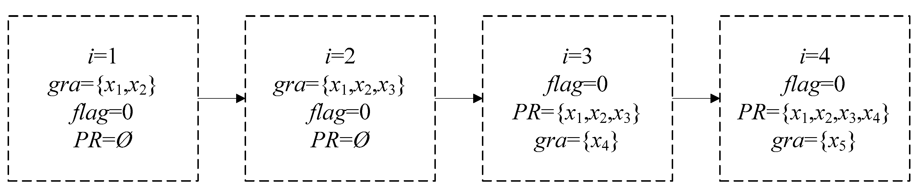
Example 2.

According to Algorithm 4, the positive region of the PR-SADT in Table 2 is calculated by the following process.

Suppose R = {a₁,a₂}. In step 1, PR=$\varnothing$, gra = {x₁}, flag =0. In step 2, these parameters were calculated in Figure 1.

In step 3, the last object x₅ is added into PR. Finally, output the positive region $PR=\{x_1,x_2,x_3,x_4,x_5\}$.

4.4. The Attribute Reduction Algorithm Based on PR-SADT

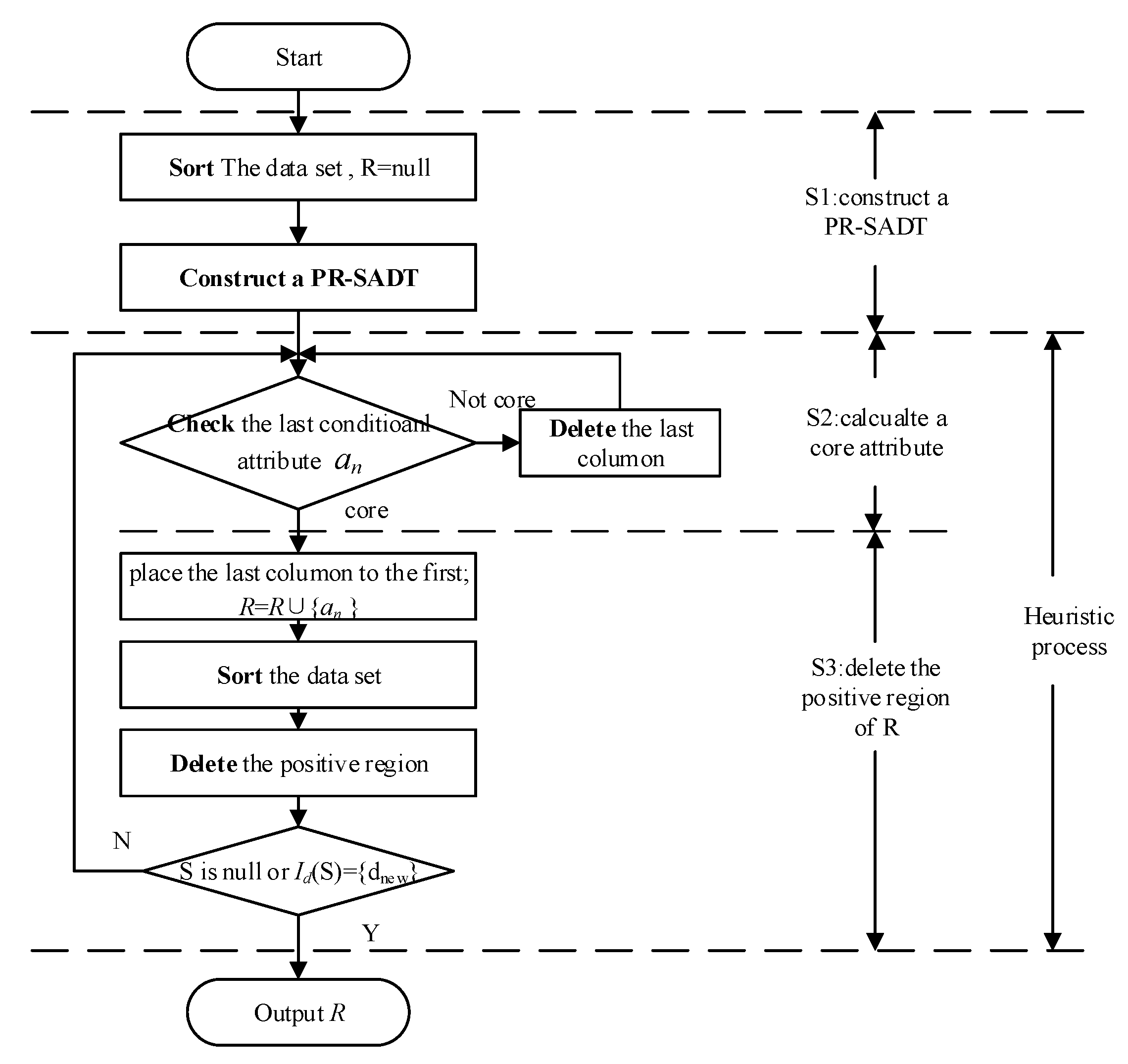
The fast positive region reduction algorithm based on PR-SADT (FPRA) was proposed as Algorithm 5, and the related flow chart is described as Figure 2.

Algorithm 5. The fast positive region reduction algorithm based on PR-SADT (FPRA)

Input: a decision table S.

Output: a complete reduct.

1: Step 1. R =$\varnothing$. Sort the original decision table.

2: Step 2. Delete the repeated objects, and calculate a PR-SADT by Algorithm 1.

3: Step 3. Check the last condition attribute an by Algorithm 2. If it is a core attribute, then jump to step 5; else, step 4.

4: Step 4. Delete the last column data, and jump to step 3.

5: Step 5. R = R∪{ak }. Place the last column to the first column, and sort the decision table.

6: Step 6. Calculate the positive region with respect to R by Algorithm 4. Delete the positive region.

7: If Sp is null or Id(Sp) is dnew, then output the reduct R; else, jump to step 3.

Analysis on the completeness of FPRA:

FPRA satisfies two key features. First, it adopts the reduct construction by deletion. Second, each attribute in R is a core attribute with respect to the related heuristic steps. Thus, R is a complete reduct.

The detail proof is described as follows.

Considering any attribute $a_i\in R$, there is a object pair (x_k,x_k+1), which satisfies the conditions according to step 3 in FPRA: (x_k,x_k+1)$\in IND\left(B\right)$, $I_{a_n}\left(x_k\right)<I_{a_n}\left(x_{k+1}\right)$, and $I_d\left(x_k\right)\ne I_d\left(x_{k+1}\right)$, where B=R_i∪{a₁,a₂,…,a_i−1}, $R_i=\left\{a_j\in R|j>i\right\}$. This means that the object pair (x_k,x_k+1) cannot be discerned by B. At the same time, owing to $R-\left\{a_i\right\}\subseteq B$, it is concluded that the object pair (x_k,x_k+1) cannot be discerned by R-{a_i}. However, the object pair can be discerned by R according to Algorithm 5. Thus, attribute a_i is essential for attribute set R.

In conclusion, the attributes of R are jointly sufficient and individually necessary for the original data set. Thus, R is a complete reduct.

Analysis on time complexity:

FPRA includes three subprocesses: the S1 process of constructing a PR-SADT (step 1 and step 2), the S2 process of calculating a core attributes (step 3->step 4->step 3) and the S3 process (step 5->step 6).

Considering an original decision table, one adopts the algorithm in [27,30] to construct a PR-SADT with the time complexity of O(|U||C|). However, the real running times of algorithms in [27,30] are dependent on the good programming style or habit. In the related experimental section, we apply the sortrows function to sort a decision table. Step 2 is accomplished by Algorithm 1, and the time complexity is O(|U||C|). Thus, the time complexity of the S1 subprocess is O(|U||C|).

In the next steps, the number of object sets and condition attribute sets are different in each heuristic process. The S2 process (step 3->step 4) deletes some related columns of data set, and the S3 process (step 5->step 6) rearranges the PR-SADT and deletes the related positive regions (some rows of data set). These two subprocesses reduce |U| and |C| and are highly efficient in optimizing the time complexity of FPRA.

Let U_i and C_i represent the object set and condition attribute set of the ith heuristic process, respectively. It has $U_1\supset U_2\supset \dots \supset U_{k-1}$,$C_1\supseteq C_2\supseteq \dots \supseteq C_{k-1}$, where k = |R| is the number of attributes in reduct R, C₁ = C, and |U₁| = |U/C|.

Step 3 is calculated with Algorithm 2, and the time complexity is O(|U_i||C_i|). Step 5 sorts the decision table, and the complexity of the ith heuristic process is O(|U_i||C_i|). The time complexity of step 6 includes two parts. One comes from Algorithm 4 and is represented as O(i |U_i|), where i is the number of attributes of R for the ith heuristic process. The other part originated by deleting the positive region, and it also has a time complexity of O(i |U_i|).

In Algorithm 5, S2 subprocess will be performed |R| times and thus has a time complexity of $O\left({{\displaystyle \sum }}_{i=1}^{\left|R\right|}\left|U_i\right|{{\displaystyle \sum }}_{j=1}^{Q_i}\left(\left|C_i\right|-j+1\right)\right)$ where Q_i = |C_i|-|C_i+1|. S3 will also be performed |R| times with time complexity of $O\left({{\displaystyle \sum }}_{i=1}^{\left|R\right|}\left|U_i\right|\left(i+\left|C_i\right|\right)\right)$.

Finally, the total time complexity is $O(|U\left|\right|C|+{\displaystyle {\sum }_{i=1}^{\left|R\right|}\left|U_i\right|}(i+\left|C_i\right|)+{\displaystyle {\sum }_{i=1}^{\left|R\right|}\left|U_i\right|}{\displaystyle {\sum }_{j=1}^{Q_i}(|C_i|-j+1)})$. In the best case where R = {c_|C|}, even the speed of O(|C||U|) is possible. In the worst case where R = C, the time complexity is $O\left(\left|U\right|\left|C\right|+{{\displaystyle \sum }}_{i=1}^{\left|C\right|}\left|U_i\right|\left(i+\left|C_i\right|\right)+{{\displaystyle \sum }}_{i=1}^{\left|C\right|}\left|U_i\right|\left|C_i\right|\right)$. Considering R is the output of FPRA, the time complexity is treated as $O(\left|U\right|\left|C\right|+{{\displaystyle \sum }}_{i=1}^{\left|C\right|}\left|U_i\right|\left(i+2\left|C_i\right|\right)$. The time complexity of FPRA is considerably less than those of traditional algorithms, which has a time complexity of O(|U|²|C|²) [2,27]. To stress the advantage of Algorithm 4, some excellent reduction algorithms are compared and listed in

Table 5. Time complexity description.

Algorithm	Time Complexity
FPRA in this paper	$O(\left|U\right|\left|C\right|+{{\displaystyle \sum }}_{i=1}^{\left|C\right|}\left|U_i\right|\left(i+2\left|C_i\right|\right)$
FSPA in [1]	$O(|U\left|\right|C|+{\displaystyle {\sum }_{i=1}^{\left|C\right|}\left|U_i\right|}(\left|C\right|-i+1))$
Algorithm in [38]	O(|C|2|U|log|U|)
IFSPA in [39]	$O(|C{|}^3\left|U\right|+{\displaystyle {\sum }_{i=1}^{\left|C\right|}({(|C|-i+1)}^2|U_i|+{(|C|-i+1)}^3|U_i|)})$
Algorithm in [2]	O(|U|2|C|2)

.

Obviously, the time complexity of FPRA is less than those of the algorithms in [2,38,39]. It is worth noting that the U_i of the algorithm in [1] is different from U_i of FPRA. This means that it is hard to compare the efficiencies of the two algorithms (algorithm in [1] and FPRA) by the time complexity in Table 5. The related experiments in Section 5 will propose the more effective evidence to represent the advantage of FPRA.

Analysis on the characteristic of FPRA:

To summarize, FPRA is complete and efficient. It has the following important features and advantages.

1.

FPRA is dependent on an efficient sort function.

FPRA just repeats a simple procedure: sort->compare->delete. Only the most efficient sort function is considered in FPRA. Thus, all the comparisons sort algorithms, such as Bubble sort (O(n²)), Shell sort (O(nlogn)), Merge sort (O(nlogn)), Quick sort (O(nlogn)), etc., are not suitable for FPRA because of the limit of O(nlogn). Instead, bucket sort algorithms are considered because their time complexities below O(nlogn). In fact, we did not pay attention to how to design a sort function because many tools or software provide the efficient sort functions. Additionally, the sortrows function or the Shuffle in MapReduce is highly recommended.

2.

FPRA does not calculate any attribute significances.

Most of traditional heuristic attribute reduction algorithms would provide a simple or complex definition to calculate attribute significances of all the condition attributes. No matter how simple the definition is, it is necessary to calculate and compare the significances of all the attributes and select the most significant attribute. This calculation process on significance would be run (2|C|-|R|+1) ×|R|/2 times if the addition construction was adopted, or (|C|+|R|+1|)×(|C|-|R|)/2 times if the deletion construction was adopted. As a comparison, the special core attribute calculation in FPRA only would be run |C| times.

3.

The heuristic method of FPRA is more efficient and concise.

The traditional heuristic algorithms include two kinds of calculation: the entire core set calculation before the heuristic process and attribute significance calculation in heuristic processes, respectively. As a comparison, FPRA only has a kind of calculation: core attribute calculation in heuristic processes. In detail, FPRA calculates a single core attribute in each heuristic process, while the traditional algorithms have to calculate the attribute significances of all the existed condition attributes.

Besides, each conditional attribute of FPRA is checked at most once. In the traditional heuristic algorithms, a conditional attribute would be checked (2|C|-|R|+1)×|R|/(2|C|) or (|C|+|R|+1|)×(|C|-|R|)/(2|C|) times in average. Therefore, FPRA is more efficient and concise than the traditional heuristic algorithms.

5. Experimental Results

In this section, we will evaluate the proposed approach (FPRA) based on several data sets from the UCI (University of California, Irvine) Repository [1,38,40,41]. The related works include performance analysis and comparison tests. All of the experiments on FPRA were conducted using a PC with Inter(R) CPU G645, 2.9 GHz and 1.81 GB memory.

Some data sets from the UCI Repository were used in the experiments as outlined in

Table 6. Description of the data sets.

	Data Set	Size |U|	Attributes |C|	Classes |Vd|
1	Dermatology	358	34	6
2	Backup_large.test	376	35	19
3	Breast-cancer-wisconsin	683	9	2
4	Tic-tac-toe	958	9	2
5	Kr_vs_kp	3196	36	2
6	mushroom	5644	22	2
7	Ticdata2000	5822	85	2
8	nursery	12960	8	5
9	Letter-recognition	20000	16	26
10	Shuttle_all	58000	9	7
11	sensorless	58509	48	11
12	Connect-4	67557	42	3
13	Ipums.la.97	70187	60	10
14	Ipums.la.99	88443	60	10
15	covertype	581012	54	7

. There are some data sets with missing values, such as Mushroom and Breast-cancer-wisconsin. For uniform treatment of all data sets, we replaced the missing values with a new value that did not appear in the original data set. Some data sets, such as sensorless, were transformed into discrete data sets by a simple uniform discretization algorithm. Specifically, each of the related continuous columns was divided into 10 equal intervals.

5.1. Performance Analysis

At present, the time complexities of fast reduction algorithms have beyond O(|U||C|²) and entered the interval of (O(|U||C|), O(|U||C|²)). In order to illustrate the advantages on computational efficiency, many researchers have to apply some inexact and sealed parameters, such as U_i, C_i, etc., to describe the time complexities of proposed algorithms. These time complexities suffer two disadvantages.

• It is difficult to estimate the real running times from the time complexities using sealed parameters. For example, the time complexity of the fast reduction algorithm in [1] is $O(|U\left|\right|C|+{\displaystyle {\sum }_{i=1}^{\left|C\right|}\left|U_i\right|}(\left|C\right|-i+1))$. It is less than O(|U||C|²). However, there are |C| sealed parameters |U₁|,|U₂|,…,|U_|C||. It is hard to estimate the exact running time.
• It is difficult to compare the computational efficiencies of different reduction algorithms. First, these sealed parameters are influenced by the heuristic constructions and real data sets. They have different values for different algorithms. Second, the time complexities with these sealed parameters are always very complex, such as FSPA, etc.

In this paper, the proposed algorithm FPRA is also confused by the above hard problems. It has some sealed parameters, which are U₁,U₂,..,U_|R|,C₁,C₂,…,C_|R|, respectively. It is very difficult to estimate the real efficiency based on the theoretical time complexity of $O(\left|U\right|\left|C\right|+{{\displaystyle \sum }}_{i=1}^{\left|C\right|}\left|U_i\right|\left(i+2\left|C_i\right|\right)$. In order to resolve these hard problems, we suggest an approximate time complexity of FPRA, which is simple and easy to estimate the real running time. The detailed way is described as follows.

We will record the real running times of three subprocesses of FPRA and analyze the features of subprocesses. On the basis, an experimental model of time complexity is suggested.

Some classical data sets in UCI are applied to test the related running time and the experimental results are listed in

Table 7. The time consumption of subprocess of FPRA.

	Data Set	|U|	|R|/|C|	Time of S1 T1(s)	Time of S2 T2(s)	Time of S3 T3 (s)	Total Time T(s)
1	mushroom	5644	7/22	0.047	0.031	0.079	0.157
2	Ticdata2000	5822	24/85	0.078	0.251	0.624	0.953
3	nursery	12960	8/8	0.062	0	0.266	0.328
4	Letter-recognition	20000	12/16	0.109	0.062	0.375	0.546
5	Shuttle_all	58000	4/9	0.235	0.078	0.516	0.829
6	sensorless	58509	39/48	0.828	0.592	6.907	8.327
7	Connect_4	67557	34/42	0.719	1.143	14.967	16.829
8	Ipums.la.97	70187	8/60	0.750	1.657	1.328	3.735
9	Ipums.la.99	88443	13/60	0.906	2.311	2.424	5.641
10	covertype	581012	6/54	4.140	39.25	6.078	49.468

, where T₁, T₂, and T₃ are the running time with respect to the three subprocesses of S1, S2, and S3, respectively.

Especially, the covertype data set was seldom reported by the existing reduction algorithms because of 581,012 objects and 54 attributes. However, FPRA could calculate this data set within only 49.468 s. This phenomenon means that FPRA was efficient to the existing reduction algorithms. Some ratios on the time consumption of subprocesses are presented in Figure 3.

Figure 3 describes the ratios of |R|/|C|, T₂/T, and T₃/T, where the X-coordinate represents the ten data sets in Table 7, and T₁, T₂, and T₃ are the running time with respect to the three subprocesses of S1, S2, and S3, respectively. Some important conclusions are presented as follows.

• The S3 subprocess consumed the most running time when |R|/|C| was large. For data sets (3,4,6,7), the ratios of |R|/|C| were 1, 0.75, 0.8125, and 0.8095, respectively. The related ratios of T₃/T were 0.811, 0.6868, 0.8295, and 0.8894.
• The S2 subprocess consumed the most running time when |R|/|C| was small. For data sets (8, 10), the ratios of |R|/|C| were 13.3% and 11.1%, respectively. The related ratios of T₂/T were 44.36% and 79.34%.
• The trend of T₃/T was similar to that of |R|/|C|; the trend of T₂/T was opposite to that of |R|/|C|.

The above features show that the real running time was influenced by |R| as well as |U| and |C|.

Next, we compared the time complexity of FPRA with O(|U||C|²) and O(|U||C||R|). The related results are presented in Figure 4.

The time complexity of S1 was O(|U||C|). Suppose the real time complexity of FPRA is similar to O(k|U||C|). Then, k is described as the ratio of T/T₁. In Figure 4, the ratios of T/T₁ varied from 3.34 to 23.4, and the average value was 8.6. As a comparison, the average value of |C| was 40.4. Obviously, the time complexity of FPRA was considerably less than O(|U||C|²). The average value of |R| was 15.5, which was slightly more than that of the ratios of T/T₁.

As a result, the real time complexity of FPRA is similar to O(|U||C||R|).

To obtain more accurate experimental results, we constructed 60 data sets based on six original data sets, which were shuttle_all, sensorless, connect_4, ipums.la.97, ipums.la.99, and covertype, respectively. For each original data set, we divided it into 10 parts of equal size. The first part was regarded as the first data set, the combination of the 1st part and the 2nd part was viewed as the second data set, and the combination of all ten parts was viewed as the tenth data set.

The related ratios for the real running time of the 60 data sets are shown in Figure 5.

In the 60 data sets in Figure 5, S3 consumed the most running time (T₃/T > 50%) when |R|/|C| > 40%. S2 consumed the most time (T₂/T > 50%) when |R|/|C| < 20%. In all of the subfigures, it was easy to determine that the trend of T₂/T was opposite to those of T₃/T. These features show that the real running time had a tight relationship with |R|.

Next, we evaluated the real time complexity with the 60 data sets.

In the 60 data sets in Figure 6, the curves on |C| were higher than the other curves. This shows that the real time complexity of FPRA was considerably less than O(|U||C|²). There were 46 data sets that had |R| > T/T₁. The other 14 data sets satisfied the condition that |R| < T/T₁. The average value of |C| for the 60 data sets was 45.5. As a comparison, the average values of T/T₁ and |R| of the 60 data sets were 9.2252 and 15.3, respectively. In particular, in shuttle_all, ipums97, and ipums99 data sets, the curves of |R| and T/T₁ were very similar.

As a result, the real time complexity of FPRA could be evaluated as O(|U||C||R|), which was less than O(|U||C|²). It is noted that O(|U||C||R|) was an experimental result, not a theoretical result.

5.2. Comparison Experiments

To illustrate the advantage of FPRA, it was compared with some existing fast reduction algorithms, which also calculated a positive region-based reduct.

In order to obtain fair and objective conclusion, all the running times of compared algorithms were recorded from the related literatures. That is, the running times of compared algorithms were proved by the original researchers. At the same time, we used the similar PC and the same data sets to obtain the real running times of FPRA. This method avoids the influences on programming habits of researchers and makes the conclusion objective.

Experiment 1.

It was compared with the classical reduction algorithm and the optimized algorithm in [1]. The experimental results are listed in

Table 8. Comparison results with PR and FSPA-PR.

Data Sets	|U|	|C|	PR		FSPA-PR		FPRA
			Time (s)	|R|	Time (s)	|R|	Time (s)	|R|
Dermatology	358	34	0.8438	10	0.4375	10	0.016	11
Backup_large.test	376	35	0.6563	10	0.4219	10	0.016	9
Breast-cancer-wisconsin	683	9	0.1250	4	0.0938	4	0.016	5
Tic-tac-toe	958	9	0.3594	8	0.3125	8	0.031	8
Kr_vs_kp	3196	36	28.0313	29	21.5781	29	0.407	29
Mushroom	5644	22	24.875	3	20.4531	3	0.157	7
Ticdata2000	5822	85	886.4531	24	296.375	24	0.953	24
Letter-recognition	20000	16	282.6406	11	112.625	11	0.546	8
Shuttle_all	58000	9	906.0625	4	712.25	4	0.829	4

.

PR is a classical reduction algorithm based on a positive region, and FSPA-PR is an optimized reduction algorithm proposed in [29]. The running times of PR and FSPA-PR are recorded from the literature [1].

In Table 8, three reducts of FPRA were larger than those of PR, and two reducts (Backup_large.test and Letter-recognition) were less than those of PR. This is due to the different heuristic construction. FPRA is based on reduct construction by deletion, while PR and FSPA-PR were based on reduct construction by addition. In [33], we noted that the reduct construction by deletion had a strong conservative property. As the price for obtaining a complete reduct, the construction by deletion was less effective in obtaining a minimal reduct.

In Table 8, FPRA clearly exhibited the best time efficiency on the nine datasets, and PR performed the worst. The ratios of running time on FPRA/PR varied from 0.09% to 12.8%. The other ratios of FPRA/FSPA-PR were from 0.12% to 17.6%. On average, for the nine data sets, the time consumption of FPRA was 0.14% of that of PR and 0.26% of that of FSPA-PR. The results show that the proposed algorithm FPRA was surprisingly efficient.

Experiment 2.

The proposed algorithm was also compared with algorithms in [38], and the results are shown in

Table 9. Comparison results with the fast algorithms in [38].

Data Sets	|U|	|C|	Running Time(s)
			ADM	OADM	FPRA
Voting records	435	16	1.375	0.171	0.015
Breast Cancer Wisconsin	683	9	2.437	0.093	0.016
Tic-tac-toe	958	9	4	0.136	0.031
Kr-vs-kp	3196	36	79.719	6.169	0.407
nursery	12960	8	1032.25	10.312	0.328

.

Algorithm ADM (Algorithm based on discernibility matrix) is a classical reduction algorithm based on the discernibility matrix and discernibility function. Its complexity is O(|U|²|C|²). Algorithm OADM (optimized ADM) is an optimized fast reduction algorithm proposed in [38], which has the complexity of O(|C|²|U|log|U|).

Table 9 shows that the running time of FPRA was considerably less than those of the compared algorithms. The ratios of running time of FPRA/ADM were only from 0.03% to 1.09%. The other ratios of FPRA/OADM were from 3.18% to 27.79%. On average, for the five data sets, the time consumption of FPRA was 0.071% of Algorithm ADM and 4.72% of Algorithm OADM.

Experiment 3.

We compared FPRA with the reduction algorithm in [40], and the results are shown in

Table 10. Comparison results with Q-ARA in [40].

Data Sets	Objects |U|	Attributes |C|	Classes |Vd|	Running Time(s)
				Q-ARA	FPRA
waveform	5000	21	3	16.466	0.156
Wine recognition	178	13	3	0.182	0.016
Statlog heart	270	13	2	0.275	0.015
Statlog project satellite image	6435	36	6	82.812	0.281
Image segmentation	2310	19	7	2.180	0.047
Pima indians diabets	768	8	2	0.103	0.015
wdbc	569	30	2	2.226	0.032
wpbc	198	34	2	1.328	0
Sonar, mines vs. rocks	208	60	2	0.312	0.031
Glass identification	214	9	7	0.118	0
ionosphere	351	34	2	2.211	0.015

.

It is noted that the running times of Q-ARA (Quick Assignment Reduction Algorithm) were reported by the literature [40] and tested in similar PC. Table 10 shows that the running time of FPRA was considerably less than that of Q-ARA. The ratios of running time of FPRA/Q-ARA were only from 0 to 14.56%. On average, for the 11 data sets, the time consumption of FPRA was 0.56% of Algorithm Q-ARA.

6. Conclusions

In this paper, we proposed a unique and innovative heuristic method, which applies a special core attribute calculation to replace the traditional attribute significance calculation. This method was concise and each conditional attribute was only checked at most once.

The key of the proposed method is a sort function, and the surprisingly running efficiency of FPRA is dependent on the sortrows function. The T₁ of Table 7 lists the exact times on sorting the original data and constructing a PR-SADT.

The experimental analysis shows that the real time complexity of FPRA was less than O(|U||C|²).

The proposed algorithm FPRA is also appropriate for big data reduction because it only uses two basic operations (sort and comparison), while MapReduce (model for big data) provides an efficient sort technology. This issue will be addressed in future work.

References

1. Qian, Y.H.; Liang, J.Y.; Pedrycz, W.; Dang, C.Y. Positive approximation: An accelerator for attribute reduction in rough set theory. Artif. Intell. 2010, 174, 597–618. [Google Scholar] [CrossRef] [Green Version]
2. Hu, Q.H.; Liu, J.F.; Yu, D.R. Mixed feature selection based on granulation and approximation. Knowl. Based Syst. 2008, 21, 294–304. [Google Scholar] [CrossRef]
3. Wang, G.Y.; Ma, X.A.; Yu, H. Monotonic uncertainty measures for attribute reduction in probabilistic rough set model. Int. J. Approx. Reason. 2015, 59, 41–67. [Google Scholar] [CrossRef]
4. Chang, S. A novel attribute reduction method based on rough sets and its application. Int. J. Adv. Comput. Technol. 2012, 4, 99–104. [Google Scholar]
5. Hu, Q.H.; Yu, D.R.; Xie, Z.X. Neighborhood classifiers. Expert Syst. Appl. 2008, 34, 866–876. [Google Scholar] [CrossRef]
6. Liang, J.; Wang, F.; Dang, C.; Qian, Y. An efficient rough feature selection algorithm with a multi-granulation view. Int. J. Approx. Reason. 2012, 53, 912–926. [Google Scholar] [CrossRef] [Green Version]
7. Nie, S.Z.; Wang, Z.; Pujia, W.; Nie, Y.; Lu, P. Big data prediction of durations for online collective actions based on peak’s timing. Phys. A-Stat. Mech. Appl. 2018, 492, 138–154. [Google Scholar] [CrossRef]
8. Skowron, A.; Jankowski, A.; Swiniarski, R. 30 Years of Rough Sets and Future Perspectives, Rough Sets, Fuzzy Sets, Data Mining, and Granular Computing; Springer: Berlin/Heidelberg, Germany, 2013; pp. 1–10. [Google Scholar]
9. Zong, F.; Tian, Y.D.; He, Y.N.; Tang, J.J.; Lv, Y.Y. Trip destination prediction based on multi-day GPS data. Phys. A-Stat. Mech. Appl. 2019, 515, 258–269. [Google Scholar] [CrossRef]
10. Yin, L.; Gui, W.; Yang, C.; Wang, X.; Ling, C.X. Core set analysis in inconsistent decision tables. Inf. Sci. 2013, 241, 138–147. [Google Scholar] [CrossRef]
11. Deng, S.; Yue, D.; Fu, X.; Zhou, A.H. Security risk assessment of cyber physical power system based on rough set and gene expression programming. IEEE/CAA J. Autom. Sin. 2015, 2, 431–439. [Google Scholar]
12. Hu, Q.; Xie, Z.; Yu, D. Hybrid attribute reduction based on a novel fuzzy-rough model and information granulation. Pattern Recognit. 2007, 40, 3509–3521. [Google Scholar] [CrossRef]
13. Yang, M.; Yang, P. Algorithms based on general discernibility matrix for computation of a core and attribute reduction. Control Decis. 2008, 23, 1049–1054. [Google Scholar]
14. Yao, Y.Y.; Zhao, Y. Discernibility matrix simplification for constructing attribute reducts. Inf. Sci. 2009, 179, 867–882. [Google Scholar] [CrossRef] [Green Version]
15. Lu, Z.; Qin, Z.; Zhang, Y.; Fang, J. A fast selection approach based on rough set boundary regions. Pattern Recognit. Lett. 2014, 36, 81–88. [Google Scholar] [CrossRef]
16. Qian, Y.; Liang, J. Combination entropy and combination granulation in rough set theory. Int. J. Uncertain. Fuzziness Knowl. Based Syst. 2008, 16, 179–193. [Google Scholar] [CrossRef]
17. Wang, C.; Ou, F.F. An attribute reduction algorithm based on conditional entropy and frequency of attributes. In Proceedings of the International Conference on Intelligent Computation Technology and Automation, Changsha, China, 20–22 October 2008; pp. 752–756. [Google Scholar]
18. Wang, G.Y.; Zhao, J.; An, J.J.; Wu, Y. A comparative study of algebra viewpoint and information viewpoint in attribute reduction. Fundam. Inform. 2005, 68, 289–301. [Google Scholar]
19. Qian, J.; Miao, D.; Zhang, Z.; Yue, X. Parallel attribute reduction algorithms using MapReduce. Inf. Sci. 2014, 279, 671–690. [Google Scholar] [CrossRef]
20. Shu, W.H.; Qian, W.B. An incremental approach to attribute reduction from dynamic incomplete decision systems in rough set theory. Data Knowl. Eng. 2015, 100, 116–132. [Google Scholar] [CrossRef]
21. Yin, L.Z.; Yang, C.H.; Wang, X.L.; Gui, W.H. An incremental algorithm for attribute reduction based on labeled discernibility matrix. Acta Autom. Sin. 2014, 40, 397–403. [Google Scholar]
22. Yao, Y.Y. Duality in rough set theory based on the square of opposition. Fundam. Inform. 2013, 127, 49–64. [Google Scholar] [CrossRef]
23. Chen, Y.M.; Miao, D.Q.; Wang, R.Z. A rough set approach to feature selection based on ant colony optimization. Pattern Recognit. Lett. 2010, 31, 226–233. [Google Scholar] [CrossRef]
24. Yang, P.; Li, J.; Huang, Y. An attribute reduction algorithm by rough set based on binary discernibility matrix. In Proceedings of the Fuzzy Systems and Knowledge Discovery, Jinan, China, 18–20 October 2008; pp. 276–280. [Google Scholar]
25. Xu, Z.Y.; Yang, B.R.; Song, W. Quick computing core algorithm based on discernibility matrix. Comput. Eng. Appl. 2006, 42, 4–6. [Google Scholar]
26. Yang, M.; Sun, Z.H. Improvement of discernibility matrix and the computation of a core. J. Fudan. Univ. 2004, 43, 865–868. [Google Scholar]
27. Xu, Z.Y.; Shu, W.H.; Qian, W.B.; Yang, B.Y. Quick algorithm for computing core of the positive region based on order relation. Comput. Sci. 2010, 37, 208–211. [Google Scholar]
28. Liu, S.H.; Sheng, Q.J.; Wu, B.; Shi, Z.; Hu, F. Research on efficient algorithms for rough set methods. Chin. J. Comput. 2003, 26, 524–529. [Google Scholar]
29. Shen, J.; Lv, Y. A rapid algorithm for reduction based on positive region attribute significance. In Proceedings of the Electrical and Control Engineering (ICECE), 2010 International Conference on, Wuhan, China, 25–27 June 2010; pp. 4940–4943. [Google Scholar]
30. Xu, Z.Y.; Liu, Z.P.; Yang, B.R.; Song, W. A Quick Attribute reduction algorithm with complexity of max (O(|C||U|,O(|C|2|U/C|))). Chin. J. Comput. 2006, 29, 391–399. [Google Scholar]
31. Zhang, J.; Zhang, X.Y.; Xu, W.H. Lower approximation reduction based on discernibility information tree in inconsistent ordered decision information systems. Symmetry 2018, 10, 696. [Google Scholar] [CrossRef] [Green Version]
32. Zhao, Y.; Yao, Y.Y.; Luo, F. Data analysis based on discernibility and indiscernibility. Inf. Sci. 2007, 177, 4959–4976. [Google Scholar] [CrossRef]
33. Yin, L.Z.; Yang, C.H.; Wang, X.L.; Gui, W.-H. Reduction method based on attribute repulsion matrix. Control Decis. 2013, 28, 434–438. [Google Scholar]
34. Witold, P. Granular computing for data analytics: a manifesto of human-centric computing. IEEE/CAA J. Autom. Sin. 2018, 5, 1025–1034. [Google Scholar]
35. Qian, J.; Miao, D.; Zhang, Z.; Li, W. Hybrid approaches to attribute reduction based on indiscernibility and discernibility relation. Int. J. Approx. Reason. 2011, 52, 212–230. [Google Scholar] [CrossRef] [Green Version]
36. Yao, Y.Y.; Zhao, Y.; Wang, J. On reduct construction algorithms. In Rough Sets and Knowledge Technology; Springer: Berlin/Heidelberg, Germany, 2006; pp. 297–304. [Google Scholar]
37. Jehad, A.; Rami, M. An enhancement of major sorting algorithms. Int. Arab J. Inf. Technol. 2010, 7, 55–62. [Google Scholar]
38. Meng, Z.; Shi, Z. A fast approach to attribute reduction in incomplete decision systems with tolerance relation-based rough sets. Inf. Sci. 2009, 179, 2774–2793. [Google Scholar] [CrossRef]
39. Qian, Y.; Liang, J.; Pedrycz, W.; Dang, C. An efficient accelerator for attribute reduction from incomplete data in rough set framework. Pattern Recognit. 2011, 44, 1658–1670. [Google Scholar] [CrossRef]
40. Li, M.; Shang, C.; Feng, S.; Fan, J. Quick attribute reduction in inconsistent decision tables. Inf. Sci. 2014, 254, 155–180. [Google Scholar] [CrossRef]
41. Song, M.; Wu, Y.F. Handbook of Research on Text and Web Mining Technologies; IGI Global: Hershey, PA, USA, 2009; Chapter XLIV; pp. 766–784. [Google Scholar]
Figure 1. The calculation process of step 2 of Algorithm 4.
Symmetry 12 01189 g001
Figure 2. The flow chart of fast positive region reduction algorithm based on PR-SADT (FPRA).
Symmetry 12 01189 g002
Figure 3. The ratios of |R|/|C|, T2/T, and T3/T.
Symmetry 12 01189 g003
Figure 4. Evaluation on T/T1 of FPRA.
Symmetry 12 01189 g004
Figure 5. The ratios of |R|/|C|, T2/T, and T3/T based on 60 data sets.
Symmetry 12 01189 g005
Figure 6. Evaluation on T/T1 based on 60 data sets.
Symmetry 12 01189 g006