Review

Fractional Riccati Equation and Its Applications to Rough Heston Model Using Numerical Methods

Department of Mathematics and Institute for Mathematical Research, University Putra Malaysia, Serdang 43400, Selangor, Malaysia
*
Author to whom correspondence should be addressed.
Symmetry 2020, 12(6), 959; https://doi.org/10.3390/sym12060959
Submission received: 22 February 2020 / Revised: 14 March 2020 / Accepted: 24 March 2020 / Published: 5 June 2020
(This article belongs to the Special Issue Recent Advances in Discrete and Fractional Mathematics)

Abstract

:
Rough volatility models are recently popularized by the need of a consistent model for the observed empirical volatility in the financial market. In this case, it has been shown that the empirical volatility in the financial market is extremely consistent with the rough volatility. Currently, fractional Riccati equation as a part of computation for the characteristic function of rough Heston model is not known in explicit form and therefore, we must rely on numerical methods to obtain a solution. In this paper, we will be giving a short introduction to option pricing theory (Black–Scholes model, classical Heston model and its characteristic function), an overview of the current advancements on the rough Heston model and numerical methods (fractional Adams–Bashforth–Moulton method and multipoint Padé approximation method) for solving the fractional Riccati equation. In addition, we will investigate on the performance of multipoint Padé approximation method for the small u values in D α h ( u i / 2 , x ) as it plays a huge role in the computation for the option prices. We further confirm that the solution generated by multipoint Padé (3,3) method for the fractional Riccati equation is incredibly consistent with the solution generated by fractional Adams–Bashforth–Moulton method.

1. Introduction

The classical stochastic volatility diffusion models such as [1,2] have played an important role in volatility modelling specifically to match for the smile or skew effect (variation of implied volatility with respect to strike price) as displayed in the empirical implied volatility [3]. However, the shortcoming of using these stochastic volatility models is their inability o generate reasonable shape for the term-structure (variation of implied volatility with respect to maturity time) in the implied volatility. Generally speaking, the classical stochastic volatility diffusion models have a skew slope of O ( 1 ) , whereas the implied volatility based on empirical observations has a skew slope of O ( τ 1 / 2 ) [4,5,6] with τ as the time to maturity, therefore they are not compatible as market models. In response to the shortcoming, the stochastic volatility jump diffusion models such as Bates model [7] were also introduced to fit the empirical short-time skew. Moderate but insufficient improvement was made to the problem by using the stochastic volatility jump diffusion model.
Recently, the academic contribution by [8] enables us to price assets accurately by considering rough volatility in our framework. The term “rough volatility” indicates that the volatility term is driven by fractional Brownian motion (fBm) [9] with Hurst exponent of 0 < H < 1 / 2 , where H controls the roughness of the fBm (the lower the H, the rougher the trajectories of fBm). Intuitively, the term “rough volatility” came from its roughness behavior or anti-persistency effect. Accordingly, the empirical findings made by [8] were possible due to the contribution from [10], where the author has displayed that the volatility in stochastic volatility model driven by the fractional Brownian motion with Hurst exponent H is capable of generating an at-the-money volatility skew of the form τ H 1 / 2 for small τ time. This subsequently motivated the authors of [8] to model volatility using fBm with Hurst parameter of 0 < H < 1 / 2 . Prior to the discovery, we wish to note that there is a good attempt made by [11]. In particular, the authors utilized Malliavin calculus techniques to obtain the short-time behavior of at-the-money implied volatility skew for the generalization of Bates model and subsequently, considered fractional stochastic volatility models that included the case of Hurst parameter H < 1 / 2 which is capable of capturing the short-time behavior of skew slopes similar to those displayed in the financial market. Furthermore, before the use of rough volatility (fractional Brownian motion with Hurst parameter 0 < H < 1 / 2 ), authors of [12] have proposed the fractional stochastic volatility model with Hurst parameter of H > 1 / 2 , where it intends to capture the long memory effect displayed by the assets movement in the financial market. Subsequently, the stochastic volatility model with mixed fractional Brownian motion [13] was also proposed as an attempt to model assets movement better.
After the discovery of rough volatility, rough Heston model and its characteristic function have been proposed and derived in [14] by continuing the work of [15] where they have found that microscopic model for the price of an asset with leverage effect follows the rough Heston model. Coincidentally, it is found that the classical Riccati equation in the classical Heston model [2] has been replaced with fractional Riccati equation in the rough Heston model. Unlike the classical version of Riccati equation where the exact solution exists and the solution for the classical Heston can be obtained easily in an efficient manner, there is no explicit-form solution for the fractional Riccati equation as of now. This poses a huge disadvantage to use the rough Heston model for obtaining the call option price as we have to rely on numerical methods now. Unfortunately, it is also noted that to acquire an accurate solution, the computational costs originated from the lack of an explicit solution for the fractional Riccati equation which is a part of the characteristic function of the rough Heston model. It can be seen as a huge sacrifice for the sake of incorporating rough volatility in its framework.
Besides the direct confrontation on the computation of rough Heston model using Fourier-type method, it is possible to use hybrid Brownian semistationary (BSS) method [16] as an efficient simulation method. In particular, the method involves the usage of appropriate power function to approximate when the kernel function near zero and Riemann-sum discretization elsewhere. It is found that the hybrid BSS scheme is able to reproduce the fine properties of rough Brownian semistationary process, but practical implementation remains hard. A variance reduction technique [17] took advantage of the hybrid BSS scheme for obtaining the solution of the rough Bergomi model. Furthermore, authors of [18] have proposed a multifactor approximation method for the fractional Riccati equation. The specification of the method involves approximating fractional Riccati equation using a n-dimensional classical Riccati equation with large n (up to n = 500 ). A similar time-efficiency method is suggested in [19] with satisfactory results for the fits to the implied volatility smiles for short maturities with lesser parameters. [20] managed to approximate the rough Heston model by using scaled “volatility of volatility” parameter in the classical Heston model. The method is somewhat extremely fast to calibrate (follows the time complexity of classical Heston model) with satisfactory accuracy. Besides that, [21] used a hybrid method that involves the Richardson–Romberg extrapolation method to approximate outside of convergence domain and a short-time series expansion. The authors noted that the hybrid method is both efficient and flexible.
Although it has only been recently discovered that the solution to the fractional Riccati equation is essential for the pricing call option, it has actually been studied extensively for general purposes by many researchers in the past. We first mention two of the most famous methods which are the Adomian decomposition method [22] and the variational iteration method [23]. Homotopy perturbation method [24] and homotopy analysis method [25] remain popular choices for approximating the analytical solutions. Other methods on approximating fractional Riccati equation include [26,27].
The usual algorithm dealing with fractional order differential equation is obtained by using the fractional Adams–Bashforth–Moulton method [28]. The error analysis is also provided in the paper. We refer to the fractional Adams–Bashforth–Moulton method as fractional Adams method from now onwards. It is noted that [14] has also demonstrated the use of fractional Adams method in its numerical application section for the rough Heston model. Although it is capable of providing extremely well solution with large time steps, the algorithm complexity to evaluate a call option is at O ( N a n 2 ) where the N a is the number of space steps used for Fourier-type method and n is the number of time steps for the fractional Adams method. The sole complexity of the algorithm makes the computation of the call option to a certain accuracy not feasible to most practitioners. We will take advantage of this method by setting a high number of time steps to compare our numerical solution later in this paper.
In this paper, we will also focus heavily on the work of [29] where it uses multipoint Padé approximants on the asymptotical solutions ( t 0 and t ) of the fractional Riccati equation and applying it to the rough Heston model. This is needed as the typical method (fractional Adams method) requires great computational effort, i.e., not feasible to most practitioners or perhaps even researchers. Before that, we wish to discuss some of the general aspects and history of Padé approximation method. Specifically, it was developed by Henri Padé in the 1890s with the constructing idea credited to Georg Frobenius where he investigated the usage of rational approximations of the power series. Coincidentally, Padé approximation turns out to be a great approximation to many application in physics, e.g., nuclear physics [30], kinetic electron model [31], quantum resonances [32] and many more [33]. We follow closely on the literature from [29], we note that the theory of convergence of Padé approximants can be found in [34]. Also, as noted in [33], one of the theorems (Montessus de Ballore’s theorem) states that if f is analytical in a ball centered at zero except for multiples of n, the sequence of { f ( m , n ) } m = 1 for a fixed n, converges uniformly to f in compact subsets omitting the poles.
Furthermore, since we are dealing with diagonal Padé approximants for our fractional Riccati equation later on, it is only fair that we mention its convergence properties too. As noted in [35], Baker–Gammel–Wills conjecture speculates that under some certain condition, the diagonal Padé approximant { f ( n , n ) } n = 1 converges uniformly to f. Taken from [34], a counterexample for the Baker–Gammel–Wills conjecture is provided. Consequently, Nutall–Pommerenke’s theorem is provided where it states that there exists a subsequence of { f ( n , n ) } n = 1 where it converges almost everywhere. Coupled with Monstessus de Ballor’s theorem, we should be extremely careful when dealing with diagonal Padé approximant in our work. One of the functions we will mention later is the Mittag–Leffler function E α ( z ) . The uniform convergence of Mittag–Leffler function has been proven in [36] on the compact set { | z | 1 } . However, it is not necessarily compatible with the asymptotic behavior of the Mittag–Leffler function for large t, although it performs better than their corresponding truncated Taylor series.
We now move to the discussion on the multipoint Padé approximation method. The method was originally derived in [37] as a global rational approximant. As mentioned previously, it aims to match asymptotical points of f using ( m , n ) Padé approximant. In addition, it has been successfully applied to both the Mittag–Leffler function [38] and generalized Mittag–Leffler function [39]. The authors of [29] demonstrated the use of global rational approximations for the fractional Riccati equation and found the excellent performance of the multipoint Padé approximation ( 3 , 3 ) especially when H is close to 0. However, the imaginary part of the solution deteriorates as H 0.5 or α 1 . This poses a challenge in terms of accuracy of the model and it would be erroneous to employ the same method to approximate the solution for the fractional Riccati equation when H is somewhat near 0.5 . In addition, we take a step further to investigate the accuracy of D α h ( u i / 2 , x ) for small u values as it plays an important role for the computation of option price. Consequently, we further confirm that the multipoint Padé (3,3) approximation method performs incredibly well at small u values as compared to fractional Adams method, thereby enabling practitioners to price their options using a low computational cost method with similar accuracy.

Organization of the Paper

We have provided a short introduction to the Riemann–Liouville fractional calculus in the Appendix A and Mittag–Leffler function in Appendix B as preliminaries for interested readers. Furthermore, we intend to organize our paper as following:
Section 2: Fractional Adams–Bashforth–Moulton method and its error analysis.
Section 3: Black Scholes equation, implied volatility, classical Heston, rough Heston model, their characteristic functions and their connection to call option pricing.
Section 4: Small and long time expansion of solution for the fractional Riccati equation.
Section 5: Padé, multipoint Padé approximation method and its application to the asymptotical solutions of the fractional Riccati equation.
Section 6: Numerical experiments and performances.

2. Fractional Adams–Bashforth–Moulton Method and Its Error Analysis

We discuss the general method of obtaining a solution for the fractional ordinary differential equations in which we will utilize this method to obtain the solution for the fractional Riccati equation later on. In particular, we refer to [40] for the fractional Adams–Bashforth–Moulton method. The original work on the error analysis belongs to [28]. Furthermore, the full algorithmic description with pseudocode can be found in [41]. It is also noted that this method is also known as one of broader method called predictor corrector method or PECE (predict-evaluate-correct evaluate). This method relies on product trapezoidal method and product rectangle method in the quadrature theory. The fractional Adams method with fractional order of α is shown as following
D α h ( a , x ) = F ( a , h ( a , x ) ) , I 1 α h ( a , 0 ) = 0
h k , 0 = j = 0 α 1 x k j j ! h 0 ( j ) + Δ α j = 0 k 1 b j k F ( a , h ( a , x j ) ) ,
h k = j = 0 α 1 x k j j ! h 0 ( j ) + Δ α j = 0 k 1 a j k F ( a , h ( a , x j ) ) = + Δ α a k k F ( a , h k . 0 )
h ( a , 0 ) = 0
with a j , k and b j , k as
a j , k = 1 Γ ( 2 + α ) × ( ( k 1 ) 1 + α ( k α 1 ) k α ) if j = 0 , ( ( k j + 1 ) 1 + α + ( k j 1 ) 1 + α ( ( k j + 1 ) 1 + α 2 ( k j ) 1 + α ) if 1 j k 1 , 1 if j = k .
b j , k = 1 Γ ( 1 + α ) ( ( k j ) α ( k 1 j ) α ) if 1 j k
In particular, we can let N = k as the total of time steps, pick T and Δ such that N = T / Δ , where T is the total time and Δ is the step size (usually extremely small). Subsequently, the  D α h ( a , x ) in Equation (1) will be our interest of study—fractional Riccati equation. It is noted that the complexity of this algorithm is at O ( N 2 ) . In the later section, we will discuss why employing this algorithm for the rough Heston model in the option pricing framework has higher computational complexity than  O ( N 2 ) .
We follow similarly from [14] and note that [42] provides convergence proofs of fractional Adams method. We denote h j as the solution obtained using fractional Adams method and h ( x j ) as the real solution. In particular, for  x > 0 and a R
max x j [ 0 , x ] | h j h ( x j ) | = O ( Δ )
and
max x j [ ε , x ] | h j h ( x j ) | = O ( Δ 2 α )
for any ε > 0 .

3. Option Pricing Models, Implied Volatility, Characteristic Functions of the Option Pricing Models

We discuss some of the financial related models and their aspects in this section. We intend to organize them as following
  • Introduce the famous Black–Scholes pricing model and discuss about implied volatility as well as its importance in the financial market.
  • Focus on one of the most famous financial model amongst the practitioners—classical Heston model and the newly developed rough Heston model.
  • Display its characteristic functions and its connection to call option pricing formula using the inversion of characteristic function.

3.1. Black–Scholes Model and Implied Volatility

The Nobel Prizes of economics were awarded to the Myron S. Scholes and Robert C. Merton in 1997 for their extremely marvellous derivation of the now known as Black–Scholes equations. Sadly, one of the authors Fisher Black passed away before receiving the prize. In this subsection, we briefly discuss about the option pricing equation [43] from the Black–Scholes equation derived under some conditions and the implied volatility. The importance of the discussion for Black–Scholes model is at its implied volatility computation. Although we will not display the usage of the implied volatility in this study, we believe that some readers would find its mechanism interesting. In particular, Black and Scholes derived the Black–Scholes equation using two different methods, i.e., constructing a hedged portfolio and the capital asset pricing. Both of which led to the same equation. We now provide the closed-form solution for the European call option:
BS ( S , K , σ , r , T ) = S N ( d 1 ) K e r T N ( d 2 ) d 1 = ln S K + ( r + σ 2 / 2 ) T σ T , d 2 = d 1 σ T
where S is the stock price, K is the strike price, σ is the volatility of the stock return, r is the interest rate, T is the time to maturity and N ( · ) is the cumulative normal density function. The short and concise Equation (9) plays an important concept in the financial industry; literally everyone who trades stock and options would have known or heard about it. However, some of the assumptions that led to Equation (9) are unrealistic. One of them is the assumption of constant volatility in which we intend to replace it with rough volatility in the rough Heston model. Nevertheless, we will discuss why Equation (9) is still popular among the practitioners.
Although no practitioners would use Equation (9) to price their options in this era, many of them took interest on its implied volatility σ i m p . The implied volatility has become the standard tool to evaluate the volatility surface of a particular stock. Volatility surface is a combination of volatility skew/smile and volatility term structure, normally seen as a three-dimensional graph for comparison purposes. Let the F m as the market price of the model or price of other option model, then
F m = BS ( S , K , σ i m p , r , T )
σ i m p = BS 1 ( F m )
with BS 1 ( F m ) denoting the inverse of market price on the Black–Scholes function in Equation (9). While there is no explicit closed form solution for obtaining Equation (10), the monotonic relationship of the Black–Scholes pricing model and the volatility σ makes the implied volatility extremely easy to obtain. The monotonicity of σ can be seen from one of the greeks of Black–Scholes pricing model—vega or C σ where C is the call option price in equation (9). In particular, bisection method is one of the easy and fast way to obtain the implied volatility σ i m p . What practitioners normally do with the implied volatility σ i m p is that they compare the figures across different strike price K and maturity T in between the volatility implied by the financial market prices and the model prices. As a result, it is easy to observe whether the model is capable of fitting the empirical data and reconstruct the surfaces of the market prices.

3.2. Classical Heston Model and Rough Heston Model

We now turn to the discussion of Heston models, both classical and rough version. Suppose from [2], we let some security or stock price S and its instantaneous variance V = σ 2 such that S and V follow the stochastic process:
d S t S t = V t { ρ d B t + 1 ρ 2 d B t }
d V t = λ ( θ V t ) d t + λ ν V t d B t
where λ 0 is the magnitude or speed of mean reversion level, θ 0 is the mean reversion level for the volatility, ν is the volatility of the volatility of the model and finally ρ [ 1 , 1 ] is the correlation between B t and B t as the independent Brownian motions. From [14], we discuss why the classical Heston model is popular among the practitioners.
  • The model reproduce several stylized facts of low frequency stock data, e.g., the leverage effect, time-varying volatility and fat tails.
  • It generates similar shapes and dynamics for the implied volatility surface.
  • Efficient computation for the classical Heston model using the explicit formula for the characteristic function of the asset log-price (we will discuss it later).
Subsequently, we discuss about the the rough volatility model shown in [14], the one-dimensional asset price S is in the form of
d S t S t = V t { ρ d B t + 1 ρ 2 d B t }
with
V u = V t + λ Γ ( H + 1 2 ) t u θ t ( s ) V s ( u s ) 1 2 H d s + λ ν Γ ( H + 1 2 ) t u V s ( u 1 2 ) 1 2 H d B s u t
where λ 0 , ρ [ 1 , 1 ] is the correlation between spot and volatility movement, Γ ( · ) is the Gamma function, ν is the volatility of the volatility, H is the so called Hurst parameter with the connection of α = H + 1 / 2 from the Appendix A and θ t ( s ) is the F t -measurable mean reversion level that makes the model time consistent [44]. We note that the third term in Equation (15) is the fractional Brownian motion with Hurst parameter H, when H is between ( 0 , 1 / 2 ) , the rough Heston model follows. In particular, the Hurst parameter controls the roughness of Brownian motion. When 0 < H < 1 / 2 , the fractional Brownian motion displays a rougher state or anti-persistency of fluctuating pattern as compared to the classical Brownian motion. Furthermore, fractional Brownian motion possesses memory property, i.e., future observation depends on the past observations, a feature seen in the financial stock market. As a result, we note that fractional Brownian motion with Hurst parameter 0 < H < 1 / 2 matches empirical volatility in the financial market better than the classical Brownian motion, therefore it is advantageous to use the rough Heston model rather than classical Heston model for modelling the dynamics of assets. Visit ([8], Figure 15) for a figure illustration on the comparison of fractional Brownian motion and the market volatility. Not surprisingly, when H = 1 / 2 , the rough Heston model will revert back to the classical Heston model.
In comparison to Equation (15), under the perfect hedging scheme as shown in [44], Equation (15) can be rewritten in the compact form of
V u = ξ t ( u ) + ν Γ ( H + 1 2 ) t u V s ( u 1 2 ) 1 2 H d B s u t
where ( ξ t ( u ) ) u t is the forward variance curve observed at time t. This is because λ θ t ( s ) can be inferred from the forward variance curve, therefore λ is set to 0 and rewritten as the forward variance form of Equation (16). Furthermore, from [20,45], it is possible to obtain the forward variance curve by differentiating the variance swap curve. In particular, by assuming continuous sample paths, the well-known fair value variance swaps can be obtained from an infinite log-strip of out-of-money options. The importance of Equation (16) cannot be emphasized enough, reduction of parameter estimation for λ and θ t ( s ) as well as an integration term help immensely in the computation or calibration aspect of the rough Heston model. Note that the absence of λ in the second term of Equation (16) is due to a different way of expressing the notation between different authors, and we will be sure to specify the appropriate form of the characteristic function in the next section accordingly.

3.3. Characteristic Functions and Their Connection to Call Option Pricing

In this subsection, we discuss both of the characteristic functions for classical Heston and rough Heston model. Subsequently, we show their connection to call option pricing. Although the characteristic function was derived in [2], we refer to [14] for an overall review for the classical Heston model. We let the characteristic function of the log-price X t = log ( S t / S 0 ) as ϕ t ( a , T ) , then it is given by
ϕ t ( a , T ) = E [ e i aX t ] = exp ( g ( a , t ) + V 0 h ( a , t ) )
and
g ( a , t ) = θ λ 0 t h ( a , s ) d s
where h is the unique solution to the following Riccati equation:
t h ( a , t ) = 1 2 a ( a + i ) + λ ( i a ρ ν 1 ) h ( a , t ) + ( θ ν ) 2 2 h 2 ( a , t ) , h ( a , 0 ) = 0
where the parameters λ , ρ , ν and θ are taken from Equations (12) and (13). The parameter a C will be used in inversion of the characteristic function later and i is the imaginary number. As stated before, Equation (19) has an explicit closed-form solution which can be easily obtained. From page 18 of [45], the solution is given as
h ( a , t ) = r 1 e d t 1 g e d t
with
d = β 2 4 Ω κ , g = r r + , a a a a a a a r ± = β ± β 2 4 Ω κ 2 γ
κ = ( θ ν ) 2 2 , β = λ ( i a ρ ν 1 ) , Ω = 1 2 a ( a + i )
Eventually, the closed-form solutions from Equations (20)–(22) enable us to price the call option price with little effort. The exact pricing formula using the inverse Fourier method will be discussed after the introduction on characteristic function for rough Heston model.
Surprisingly, the rough case of Heston model (we are referring to Equation (15) first) that corresponds to the version of Equation (19) differs with little modification to its Riccati form. The only difference is that the classical Riccati equation is replaced with a fractional Riccati equation. In a precise form, the characteristic function of the rough Heston model is as following
ϕ t ( a , T ) = E [ e i a X t ] = exp ( g 1 ( a , t ) + V 0 g 2 ( a , t ) )
and
g 1 ( a , t ) = θ λ 0 t h ( a , s ) d s , g 2 ( a , t ) = I 1 α h ( a , t )
where α = H + 1 2 , θ and λ are taken from Equation (15), whereas h is the solution for the fractional Riccati equation with the following form:
D α h ( a , t ) = 1 2 ( a 2 i a ) + λ ( i a ρ ν 1 ) h ( a , t ) + ( λ ν ) 2 2 h 2 ( a , t ) , I 1 α h ( a , 0 ) = 0 ,
with the fractional derivative D α and integral I 1 α discussed in Appendix A. All the parameters λ , ρ and ν are taken from Equation (15). Note that when α = 1 , Equation (25) reverts back to Equation (19) and the rough Heston model coincides with the classical Heston model. Unfortunately, there is no known explicit closed-form solution for the fractional Riccati equation, i.e., no closed form solution when α < 1 . Therefore, the only available choice is to rely on numerical methods. In addition, we wish to discuss another version of rough Heston model based on the work of [44] which is based upon Equation (16). We let x α = ν t α as a dimensionless quantity and from [46], the characteristic function of Equation (16) can be denoted as following
ϕ t ( a , T ) = E [ e i a X t ] = exp { i a X 0 + 0 t D α h ( a , T u ) ξ t ( u ) d u }
where h ( a , · ) as the unique continuous solution of the fractional Riccati equation with the form of
D α h ( a , x ) = 1 2 a ( a + i ) + i ρ a h ( a , x ) + 1 2 h 2 ( a , x ) , I 1 α h ( a , 0 ) = 0
where all the parameters have the same definition as from Equation (16). Note that we are using X t = log ( S t ) in Equations (26) and (27) as compared to X t = log ( S t / S 0 ) in Equations (17) and (23). From now onwards, we will focus on this second version of characteristic function for rough Heston model, i.e., Equations (26) and (27).
We have now discussed the characteristic function of both the classical Heston model and rough Heston model. Now, we turn to the inversion of the characteristic function which leads to the option price, the key aspect of this work. From [47,48,49], the call option price can be denoted in the form of
C ( S , K , T ) = S e q T 1 π S K e ( r + q ) T / 2 0 Re [ e i u k ϕ T ( u i / 2 ) ] d u u 2 + 1 4
where S is the current stock price, q is the dividend yield, T is the time to maturity, K is the strike price of the option, r is the interest rate or borrowing rate and k = log ( K S ) . Now, using Equation (28), it is possible to evaluate the call option price under the classical Heston model immediately since the explicit closed-form solution for the classical Riccati equation is available. As for the case of fractional Riccati equation in Equation (27), the typical method to solve the equation by using the fractional Adams method as shown in Section 2. The fractional Adams method has been widely employed in [14,20,29].

4. Small and Long Time Expansion of Solution for the Fractional Riccati Equation

The short and long time expansion of the solution h ( a , x ) with x α = ν t α are the key components for our efficient approximation method (Padé approximation method) for the solution of fractional Riccati equation which we will discuss in Section 5. Therefore, we take this opportunity to discuss on the expansions in this section.

4.1. Small Time Expansion on Solution of Fractional Riccati Equation

We first discuss on the work of [46], the short-time x 0 expansion of h ( a , x ) . In particular, h ( a , x ) can be represented as
h ( a , x ) = j = 0 Γ ( 1 + j α ) Γ ( 1 + ( j + 1 ) α ) β j ( a ) x ( j + 1 ) α
with
β 0 ( a ) = 1 2 a ( a + i )
β k ( a ) = 1 2 i , j = 0 k 2 𝟙 i + j = k 2 β i ( a ) β j ( a ) Γ ( 1 + i α ) Γ ( 1 + ( i + 1 ) α ) Γ ( 1 + j α ) Γ ( 1 + ( j + 1 ) α ) + i ρ a Γ ( 1 + ( k 1 ) α ) Γ ( 1 + k α ) β k 1 ( a )
where Γ ( · ) is the Gamma function. Although Equation (31) appears as a complicated set of summation, we note that only first few terms will be used in the approximation method which we will discuss in the next section. Earlier terms of Equation (31) are fairly quite manageable and easy to obtain. We wish to emphasize that the combination of small time expansion and the Padé approximation method are extremely effective and consistent in obtaining the small time solution for the fractional Riccati equation later on.

4.2. Large Time Expansion on Solution of Fractional Riccati Equation

Next, we obtain the following work from [29]. Under the expectation for lim x h ( a , x ) = r from classical Riccati solution, we expect the solution of fractional Riccati equation behaves the same way. Consequently, we approximately let h ( a , x ) to be r in one of the term in the fractional Riccati equation as the large time expansion. Subsequently, the authors managed to derive out the large time expansion for the solution of the fractional Riccati equation. We begin by noting that Equation (27) can be rewritten as
D α h ( a , x ) = 1 2 ( h ( a , x ) r ) ( h ( a , x ) r + )
with
A = a ( a + i ) ρ 2 a 2 ; r ± = i ρ a ± A
In linear form, the fractional Riccati equation is approximated as following
D α h ( a , x ) = 1 2 ( h ( a , x ) r ) ( h ( a , x ) r + ) 1 2 ( r + r ) ( h ( a , x ) r ) = A ( h ( a , x ) r )
The solution to Equation (34) is of the form
h ( a , x ) = r [ 1 E α ( A x α ) ]
where E α ( · ) is the Mittag–Leffler function denoted in Appendix A. Equation (35) is apparent from the derivation of Equation (A6). We take a proposition from [29] as:
Proposition 1.
For x R 0 and a A = { z C : Re ( z ) 0 , 1 1 ρ 2 Im ( z ) 0 } . Let h ( a , x ) = r [ 1 E α ( A x α ) ] as x , then the h ( a , x ) solves the Equation (32) up to error term of O ( | A x α | 2 ) .
Proof. 
See proposition 3.1 in [29] with the help of corollary A1. □
From Equation (A8), it motivates the authors of [29] to derive the following result:
h ( a , x ) = r k = 0 γ k x k α A k Γ ( 1 k α )
as x along with γ 0 , γ 1 , γ 2 in the forms of
γ 1 = γ 0 = 1
γ 2 = 1 + r 2 A Γ ( 1 2 α ) Γ ( 1 α ) 2
and the general recursion formula as
γ k = γ k 1 + r 2 A i , j = 1 𝟙 i + j = k γ i γ j Γ ( 1 k α ) Γ ( 1 i α ) Γ ( 1 j α )
where Equations (37)–(39) are obtained by matching coefficients using Equation (32). Equation (36) is our large time expansion for the fractional Riccati equation. We now have the necessary tools to employ the approximation method on fractional Riccati equation.

5. Multipoint Padé Approximation Method for Fractional Riccati Equation

As we have mentioned before, the main issue for the rough Heston model is at its high computational cost. Coupled with fractional Adams method, in order to compute for the option price, a computation complexity of O ( N a N 2 ) is needed, where N a is the number of space steps for Equation (28) and N arises from the use of fractional Adams method noted in Section 2. One of the important advancements for rough Heston model belongs to the use of multipoint Padé method for obtaining the fractional Riccati equation’s solution at O ( 1 ) complexity. This is a huge leap in computational aspect as [29] has shown virtually that N 20,000 would result to a satisfactory solution indifferent from the N 50,000 case. By employing the multipoint Padé method, the computational complexity of the evaluation for option price using Equation (28) reduces to only O ( N a ) , the same as the case of the classical Heston model.
We first introduce the work of [38] which concerns with the global rational approximation on  h ( a , x ) :
h ( m , n ) ( a , x ) = i = 1 m p m y m j = 0 n q n y n
where m , n N + and we make the substitution y = x α on both Equations (29) and (36). Based on the argument for [29], we note that only diagonal Padé approximation is admissible. This is due to the fact when x , Padé approximation should approach as following
h ( m , n ) ( a , x ) p m q n y m n r
where 0 < | r | < only if m = n . Notice that if m n and x , h m , n ( a , x ) will either not admit constant other than zero or does not exist (involves or ) . Furthermore, Equation (41) corresponds to an assumption we made at Section 4.2. The possibilities of choosing m = n equals to some constant is endless. However, the authors [29] have noted that m = n = 2 and m = n = 4 do not perform well for the fractional Riccati equation case. Fortunately, the case m = n = 3 does produce excellent quality of solution for the fractional Riccati equation, at least for the H 0 solution. Therefore, we will work out the case for multipoint Padé approximation method for m = n = 3 in this section. When we mention multipoint Padé approximation method, we intend to refer it as multipoint Padé approximation method using m = n = 3 for the rest of the discussion in this paper. We follow closely from the presentation of [29] on this section.
Remember that we have set y = x α for the rest of our discussion. Suppose that from Equation (29), we obtain the small time expansion in the form of
h s ( y ) = b 1 y + b 2 y 2 + b 3 y 3 + O ( y 4 )
and from Equation (36), we have the series expansion for small time on the solution of fractional Riccati equation as
h ( y ) = w 0 + w 1 y + w 2 y 2 + O 1 y 3
The Padé ( 3 , 3 ) approximation can be written as
h ( 3 , 3 ) ( y ) = p 1 y + p 2 y 2 + p 3 y 3 1 + q 1 y + q 2 y 2 + q 3 y 3
with q 0 set to 1. Matching the coefficients to Equations (29) and (36) using Padé approximation method, we have the system of equations as
p 1 = b 1 p 2 p 1 q 1 = b 2 p 1 q 1 2 p 1 q 2 p 2 q 1 + p 3 = b 3 p 3 q 3 = w 0 p 2 q 3 p 3 q 2 q 3 2 = w 1 p 1 q 3 2 p 2 q 2 q 3 p 3 q 1 q 3 + p 3 q 2 2 q 3 3 = w 2
Accordingly, we obtain the constants p 1 , p 2 , p 3 , q 1 , q 2 , q 3 as
p 1 = b 1 p 2 = b 1 3 w 1 + b 1 2 w 0 2 + b 1 b 2 w 0 w 1 b 1 b 3 w 0 w 2 + b 1 b 3 w 1 2 + b 2 2 w 0 w 2 b 2 2 w 1 2 + b 2 w 0 3 b 1 2 w 2 + 2 b 1 w 0 w 1 + b 2 w 0 w 1 + b 2 w 0 w 2 b 2 w 1 2 + w 0 3 p 3 = w 0 ( b 1 3 + 2 b 1 b 2 w 0 + b 1 b 3 w 1 b 2 2 w 1 + b 3 w 0 2 ) b 1 2 + 2 b 1 w 0 w 1 + b 2 w 0 w 2 b 2 w 1 2 + w 0 3 = w 0 q 3 q 1 = b 1 2 w 1 b 1 b 2 w 2 + b 1 w 0 2 b 2 w 0 w 1 b 3 w 0 w 2 + b 3 w 1 2 b 1 2 w 2 + 2 b 1 w 0 w 1 + b 2 w 0 w 2 b 2 w 1 2 + w 0 3 q 2 = b 1 2 w 0 b 1 b 2 w 1 b 1 b 3 w 2 + b 2 2 w 2 + b 2 w 0 2 b 3 w 0 w 1 b 1 2 w 2 + 2 b 1 w 0 w 1 + b 2 w 0 w 2 b 2 w 1 2 + w 0 3 q 3 = b 1 3 + 2 b 1 b 2 w 0 + b 1 b 3 w 1 b 2 2 w 1 + b 3 w 0 2 b 1 2 w 2 + 2 b 1 w 0 w 1 + b 2 w 0 w 2 b 2 w 1 2 + w 0 3
Note that the solutions p 1 , p 2 , p 3 , q 1 , q 2 , q 3 can be easily obtained using solve function in MATLAB in less than one second. Now that we have the required multipoint Padé method, it is time we test it against the general approach (fractional Adams method).

6. Numerical Experiment And Performances

In the previous sections, we have demonstrated the fractional Adams method and the multipoint Padé approximation method. Therefore, it is time that we conduct some numerical experiment on the fractional Riccati equation. In particular, we have decided to compare the result of the fractional Riccati equation using fractional Adams method and the multipoint Padé approximation on a different scale of the Hurst parameter H.
The parameters used in our numerical studies are as following unless specifically stated otherwise:
ν = 0.4 ; ρ = 0.65 ; N = 20 , 000
where N belongs to the time steps of fractional Adams method. Although we have given the ν value, note that if we use x in x α = ν t α as a substitute of ν and t for the fractional Adams method and multipoint Padé method, we will not directly be affected by the value ν is computation for the plotting of D α h ( a , x ) and x.
For perspective, we first display the Re ( D α h ( a , x ) ) for H = 0.05 and H = 0.499 in Figure 1. Notice that the solution for the real part of the D α h ( a , x ) performs extremely well for small H and moderate for H 0.5 
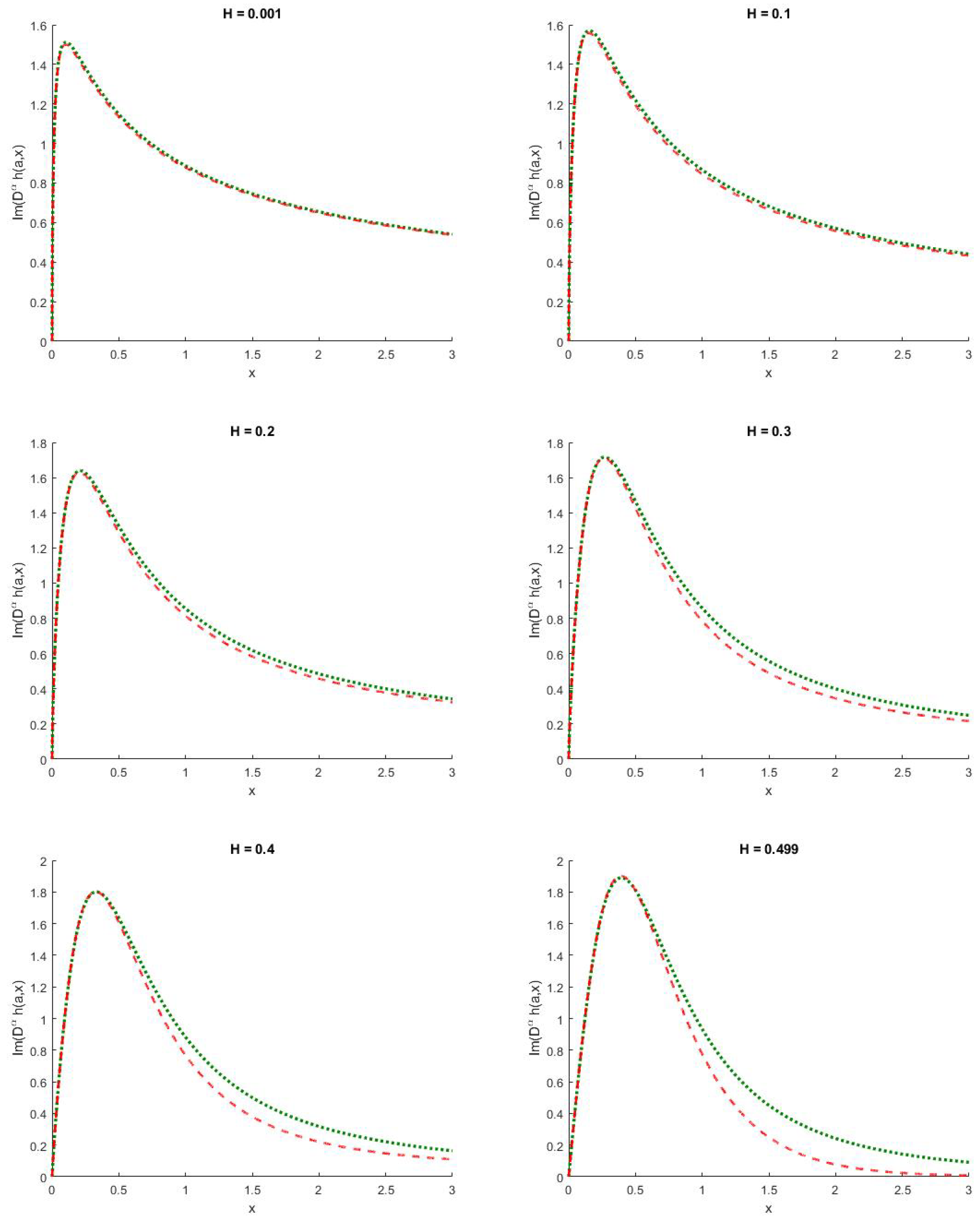
. The following observation is taken from [29]. In particular, the deterioration effect is deeply enlarged when we observe for the imaginary part of D α h ( a , x ) as seen in Figure 2. This in turn would provide an erroneous result for the option price if not fixed. In general, the performance of multipoint Padé approximation method should not be too surprising as we have matched on only two points which are x 0 and x . Supposedly, we should also understand the importance of smaller u values in ϕ T ( u i / 2 ) from Equation (28), smaller u values have higher contribution to the computation of the call option price due to the 1 / ( u 2 + 1 / 4 ) term in the integral. In the subsequent part of this section, we will evaluate D α h ( u i / 2 , x ) in a more robust setting which concerns the choices of u values at an overall scale of Hurst parameter H. We first introduce some of the notations for the purpose of computing errors.
We start with the Euclidean Norm Distance of the fractional Riccati equation’s solution:
ϵ R e H = 1 N j = 1 N Re ( D α h ^ ( u i / 2 , x j ) Re ( D α h ( u i / 2 , x j ) ) 2
ϵ I m H = 1 N j = 1 N Im ( D α h ^ ( u i / 2 , x j ) ) Im ( D α h ( u i / 2 , x j ) ) 2
and the percentage error of the fractional Riccati equation’s solution:
ε R e H = 1 N j = 1 N Re ( D α h ^ ( u i / 2 , x j ) Re ( D α h ( u i / 2 , x j ) 1
ε I m H = 1 N j = 1 N Im ( D α h ^ ( u i / 2 , x j ) Im ( D α h ( u i / 2 , x j ) 1
where u is our parameter of this study, i is the imaginary number, h ^ ( u i / 2 , x j ) is the multipoint Padé (3,3) approximation at time x j and h ( u i / 2 , x j ) is the solution at time x j generated from the fractional Adams method using parameters in Equation (46) with a slight modification of N = 3000 such that x N = 3 (we generate step size of Δ = 3 / 3000 = 0.001 ). We find that N = 3000 is a sufficient time steps for fractional Adams method with reasonable computing time. D α h is from Equation (27) and note that α = H + 1 / 2 with H as the Hurst parameter. Furthermore, Re ( · ) and Im ( · ) denote the real part and imaginary part of the solution. Equations (47) and (48) give an overall error computation of fractional Riccati equation’s solution using the multipoint Padé approximation method at different time x j up to x N = 3 , whereas Equations (49) and (50). Furthermore, in order to evaluate the quality of D α h ^ ( u i / 2 , x ) solution over different values of the Hurst parameter H, we have decided to iterate through different H for our study. Suppose we introduce χ R e , Ψ R e , χ I m , Ψ I m to achieve our final numerical computation result as follows:
χ R e = 1 50 j = 1 50 ϵ R e j / 100 , Ψ R e = 1 50 j = 1 50 ε R e j / 100
χ I m = 1 50 j = 1 50 ϵ I m j / 100 , Ψ I m = 1 50 j = 1 50 ε I m j / 100
where we iterate through H = 0.01 , 0.02 , . . . , 0.499 (we have decided to let the last H value to be 0.499 instead of 0.5). Consequently, from Table 1, we can observe that multipoint Padé approximation method does a great job in obtaining solution for various u values. Notably, χ R e and χ I m both have incredibly low values especially at u = 0.001 with virtually no errors. This is significant as it is what we needed—an accurate D α h ( u i / 2 , x ) solution at low u values. Besides, we wish to emphasize that the large errors were made by the multipoint Padé approximation method when H 0.5 whereas the market estimated Hurst parameter H values are around 0.1 [8,20]. As such, multipoint Padé approximation method would be able to perform extremely well with low computing cost. Out of the ordinary, Ψ R e and Ψ I m appear to be large across the values of u in Table 1, and upon investigation this is due to the fact that Re( D α h ( u i / 2 , x ) ) and Im( D α h ( u i / 2 , x ) ) tend to approach zero as x 3 during the computation, therefore incurring large percentage error. This is further verified by the consistent low χ R e and χ I m values. In short, the multipoint Padé approximation method performs similarly to the fractional Adams method in low computational errors manner while still retaining the low computational cost advantage.

7. Concluding Remarks

First of all, we have provided the brief history and literature review for the general stochastic volatility model, rough volatility, rough Heston model and ways to obtain solution for the rough Heston model. In particular, a large part of the literature review is dedicated to numerical methods of solving for the fractional Riccati equation where it can be used to obtain the option prices. Note that the introductory level of the fractional calculus and Mittag–Leffler function are located in the appendix for interested readers. They are subsequently used in describing the dynamics of rough Heston model and represented as the solution of fractional Riccati equation. Later, the fractional Adams–Bashforth–Moulton method and its error analysis are provided. The fractional Adams method still remains a classical and frequently used method of solving any fractional ordinary differential equation. Unfortunately, the fractional Adams method typically requires a large number of time steps which in turn requires large computational cost. But before that, we have introduced some recent advancements in the option pricing theory. Classical Black–Scholes option pricing models, classical Heston model, and the newly rough Heston models have been discussed subsequently. In addition, we gave a slight touch on the implied volatility topic in case readers are keen on testing the models on real data. Furthermore, the characteristic functions and their inversions to the option prices were given. Since the multipoint Padé approximation method requires some expansion on multiple points for matching purposes, we introduce some literature on the small and large time expansion of the solution of the fractional Riccati equation which is being used in the characteristic function of rough Heston model. We later then discuss the required multipoint Padé method ( 3 , 3 ) , as suggested by some authors, in a great effort of using the small and large time expansion to obtain the solution on fractional Riccati equation. Finally, we test the multipoint Padé ( 3 , 3 ) method on a setting and compare it with the fractional Adams method. Lastly, we have further investigated the possible outcomes on u values in D α h ^ ( u i / 2 , x ) , which is the key component in Equation (28). Consequently, the errors computation of different u values in D α h ^ ( u i / 2 , x ) further agrees that multipoint Padé ( 3 , 3 ) approximation method performs extremely consistent with the fractional Adams method. This enables practitioners to price their options with reasonable confidence such that the solution to fractional Riccati equation obtained using multipoint Padé ( 3 , 3 ) approximation method will be identical to the ones produced by the fractional Adams method, while enjoying the benefit of low computational cost. Accordingly, what we have found coincides with the previous authors such that multipoint Padé method ( 3 , 3 ) performed extremely well with H 0 but not the H 0.5 case. Above all, we wish to make a minor recommendation on this issue—since the solution for the classical Riccati equation or fractional Riccati equation with H = 0.5 exists, in our opinion, we believe it is possible for an attempt of using a hybrid model between the existing multipoint Padé method and the exact solution for the classical Riccati equation. An attempt to match it at H 0 and H 0.5 would result in a more robust setting and applicable to altering volatility behavior.

Author Contributions

Both authors have equal contribution in this article. All authors have read and agreed to the published version of the manuscript.

Funding

The authors would like to acknowledge that this research is partially supported by Special Graduate Research Allowance (SGRA) with Vote No. of 5540153.

Conflicts of Interest

It is declared that authors have no competing interests.

Appendix A. Riemann–Liouville Fractional Integrals and Fractional Derivatives

We give a brief introduction to the Riemann–Liouville fractional integrals and fractional derivatives in this section. This section is the key for understanding the discussion in Appendix B, Section 3.2 and onwards. We obtain the details of this chapter from [40] with some simplification to fit our area of study. We can define the Riemann–Liouville fractional integration for the fractional order of α ( 0 , 1 ] as
I α f ( t ) = 1 Γ ( α ) 0 t f ( s ) d s ( t s ) 1 α
and Riemann–Liouville fractional derivatives as
D α f ( t ) = d d t I 1 α f ( t ) = 1 Γ ( 1 α ) d d t 0 t f ( s ) d s ( t s ) α
with 0 t < to be the finite interval on the real axis R + and Γ ( · ) is the Gamma function. We note that when α = 1 , Equation (A2) will revert back to the classical version of differentiation.
Subsequently, we can compute the fractional derivative of x k α with fractional order α . With a little effort using change of variable along with Beta function, we can easily obtain
D α x k α = Γ ( k α + 1 ) Γ ( α ( k 1 ) + 1 ) x α ( k 1 )
Equation (A3) is important for the derivation of Equation (A6) later.

Appendix B. Mittag–Leffler Function

Following on to the discussion Mittag–Leffler function which is a crucial part in Section 4.2 for the derivation of the large time expansion on solution for fractional Riccati equation in a linearisation form. Again from [40], we define the Mittag–Leffler function of one parameter E α ( z ) for order α ( 0 , 1 ] as
E α ( z ) = k = 0 z k Γ ( α k + 1 )
with z C . An obvious deduction of E α ( A x α ) is as following
E α ( A x α ) = k = 0 A k x k α Γ ( k α + 1 )
with A C as an arbitrary constant. We note that Equation (A5) will be used as a direct application to Equation (35). Furthermore, by the relationship of Equation (A3), we obtain
D α [ E α ( A x α ) 1 ] = D α k = 1 A k x k α Γ ( k α + 1 ) + 1 1 = k = 1 A k x α ( k 1 ) Γ ( α ( k 1 ) + 1 ) = A k = 1 A k 1 x α ( k 1 ) Γ ( α ( k 1 ) + 1 ) = A E α ( A x α )
We now discuss the asymptotic expansion of Mittag–Leffler function from a review article of [50] originally taken from [51]. The rest of the discussion in this section will focus on the asymptotic expansion and its error, subsequently this discussion is important for the understanding of the large time expansion and its error behaviour in Section 4.2. From Equation (6.5) of [50], we let α ( 0 , 1 ] and μ R such that
π α 2 < μ < π α
Then for N N , N 1 , we have the asymptotic expansion as
E α ( z ) = k = 1 N 1 Γ ( 1 k α ) 1 z k + O 1 | z | N + 1 , | z | , μ | arg ( z ) | π
From Lemma B.2. and Corollary B.1. of [29], we have
Lemma A1.
For α ( 0 , 1 ] . Let a = u + i y with R 0 and i as the imaginary number, y 1 / ( 1 ρ 2 ) , 0 and let A = a ( a + i ) ρ 2 a 2 , Then for any x R > 0
| arg ( A x α ) | 3 π 4 , π
By setting μ = 3 4 π α in Equation (A8), it follows from Lemma A1 that
Corollary A1.
For α ( 0 , 1 ] . Let a = u + i y with R 0 , y 1 / ( 1 ρ 2 ) , 0 and let A = a ( a + i ) ρ 2 a 2 , Then for any x R > 0 and N N
E ( A x α ) = k = 1 N ( 1 ) k 1 A k x k α Γ ( 1 k α ) + O 1 | A x α | N + 1

References

  1. Hull, J.; White, A. The pricing of options on assets with stochastic volatilities. J. Financ. 1987, 42, 281–300. [Google Scholar] [CrossRef]
  2. Heston, S.L. A closed-form solution for options with stochastic volatility with applications to bond and currency options. Rev. Financ. Stud. 1993, 6, 327–343. [Google Scholar] [CrossRef] [Green Version]
  3. Renault, E.; Touzi, N. Option hedging and implied volatilities in a stochastic volatility model 1. Math. Financ. 1996, 6, 279–302. [Google Scholar] [CrossRef]
  4. Lee, R.W. Implied volatility: Statics, dynamics, and probabilistic interpretation. In Recent Advances in Applied Probability; Springer: Berlin, Germany, 2005; pp. 241–268. [Google Scholar]
  5. Lewis, A.L. Option Valuation under Stochastic Volatility II; Finance Press: Newport Beach, CA, USA, 2009. [Google Scholar]
  6. Medvedev, A.; Scaillet, O. Approximation and calibration of short-term implied volatilities under jump-diffusion stochastic volatility. Rev. Financ. Stud. 2007, 20, 427–459. [Google Scholar] [CrossRef] [Green Version]
  7. Bates, D.S. Jumps and stochastic volatility: Exchange rate processes implicit in deutsche mark options. Rev. Financ. Stud. 1996, 9, 69–107. [Google Scholar] [CrossRef]
  8. Gatheral, J.; Jaisson, T.; Rosenbaum, M. Volatility is rough. Quant. Financ. 2018, 18, 933–949. [Google Scholar] [CrossRef]
  9. Mandelbrot, B.B.; Van Ness, J.W. Fractional Brownian motions, fractional noises and applications. SIAM Rev. 1968, 10, 422–437. [Google Scholar] [CrossRef]
  10. Fukasawa, M. Asymptotic analysis for stochastic volatility: Martingale expansion. Financ. Stoch. 2011, 15, 635–654. [Google Scholar] [CrossRef] [Green Version]
  11. Alòs, E.; León, J.A.; Vives, J. On the short-time behavior of the implied volatility for jump-diffusion models with stochastic volatility. Financ. Stoch. 2007, 11, 571–589. [Google Scholar] [CrossRef] [Green Version]
  12. Comte, F.; Renault, E. Long memory in continuous-time stochastic volatility models. Math. Financ. 1998, 8, 291–323. [Google Scholar] [CrossRef]
  13. Cheridito, P. Mixed fractional Brownian motion. Bernoulli 2001, 7, 913–934. [Google Scholar] [CrossRef]
  14. El Euch, O.; Rosenbaum, M. The characteristic function of rough Heston models. Math. Financ. 2019, 29, 3–38. [Google Scholar] [CrossRef] [Green Version]
  15. El Euch, O.; Fukasawa, M.; Rosenbaum, M. The microstructural foundations of leverage effect and rough volatility. Financ. Stoch. 2018, 22, 241–280. [Google Scholar] [CrossRef] [Green Version]
  16. Bennedsen, M.; Lunde, A.; Pakkanen, M.S. Hybrid scheme for Brownian semistationary processes. Financ. Stoch. 2017, 21, 931–965. [Google Scholar] [CrossRef] [Green Version]
  17. McCrickerd, R.; Pakkanen, M.S. Turbocharging Monte Carlo pricing for the rough Bergomi model. Quant. Financ. 2018, 18, 1877–1886. [Google Scholar] [CrossRef] [Green Version]
  18. Abi Jaber, E.; El Euch, O. Multifactor Approximation of Rough Volatility Models. SIAM J. Financ. Math. 2019, 10, 309–349. [Google Scholar] [CrossRef] [Green Version]
  19. Abi Jaber, E. Lifting the Heston model. Quant. Financ. 2019, 19, 1995–2013. [Google Scholar] [CrossRef]
  20. El Euch, O.; Gatheral, J.; Rosenbaum, M. Roughening Heston. Available online: https://ssrn.com/abstract=3116887 (accessed on 25 March 2019).
  21. Callegaro, G.; Grasselli, M.; Pages, G. Rough but not so tough: Fast hybrid schemes for fractional Riccati equations. arXiv 2018, arXiv:1805.12587. [Google Scholar]
  22. Momani, S.; Shawagfeh, N. Decomposition method for solving fractional Riccati differential equations. Appl. Math. Comput. 2006, 182, 1083–1092. [Google Scholar] [CrossRef]
  23. Odibat, Z.; Momani, S. Application of variational iteration method to nonlinear differential equations of fractional order. Int. J. Nonlinear Sci. Numer. Simul. 2006, 7, 27–34. [Google Scholar] [CrossRef]
  24. Odibat, Z.; Momani, S. Modified homotopy perturbation method: Application to quadratic Riccati differential equation of fractional order. Chaos Solitons Fractals 2008, 36, 167–174. [Google Scholar] [CrossRef]
  25. Cang, J.; Tan, Y.; Xu, H.; Liao, S.J. Series solutions of non-linear Riccati differential equations with fractional order. Chaos Solitons Fractals 2009, 40, 1–9. [Google Scholar] [CrossRef]
  26. Jafari, H.; Tajadodi, H.; Matikolai, S.H. Homotopy perturbation pade technique for solving fractional Riccati differential equations. Int. J. Nonlinear Sci. Numer. Simul. 2010, 11, 271–276. [Google Scholar] [CrossRef]
  27. Raja, M.A.Z.; Khan, J.A.; Qureshi, I.M. A new stochastic approach for solution of Riccati differential equation of fractional order. Ann. Math. Artif. Intell. 2010, 60, 229–250. [Google Scholar] [CrossRef]
  28. Diethelm, K.; Ford, N.J.; Freed, A.D. Detailed error analysis for a fractional Adams method. Numer. Algorithms 2004, 36, 31–52. [Google Scholar] [CrossRef] [Green Version]
  29. Gatheral, J.; Radoicic, R. Rational approximation of the rough Heston solution. Int. J. Theor. Appl. Financ. 2019, 22, 1950010. [Google Scholar] [CrossRef]
  30. Thompson, I.J. Coupled reaction channels calculations in nuclear physics. Comput. Phys. Rep. 1988, 7, 167–212. [Google Scholar] [CrossRef]
  31. Lanti, E.; Dominski, J.; Brunner, S.; McMillan, B.; Villard, L. Padé Approximation of the Adiabatic Electron Contribution to the Gyrokinetic Quasi-Neutrality Equation in the ORB5 Code; Journal of Physics: Conference Series; IOP Publishing: Bristol, UK, 2016; Volume 775, p. 012006. [Google Scholar]
  32. Rakityansky, S.; Sofianos, S.; Elander, N. Pade approximation of the S-matrix as a way of locating quantum resonances and bound states. J. Phys. A Math. Theor. 2007, 40, 14857. [Google Scholar] [CrossRef] [Green Version]
  33. Baker, G.A.; Baker, G.A., Jr.; Graves-Morris, P.; Baker, S.S. Padé Approximants; Cambridge University Press: Cambridge, UK, 1996; Volume 59. [Google Scholar]
  34. Lubinsky, D.S. Rogers-Ramanujan and the Baker-Gammel-Wills (padé) conjecture. Ann. Math. 2003, 157, 847–889. [Google Scholar] [CrossRef]
  35. Lubinsky, D.S. Reflections on the Baker–Gammel–Wills (Padé) Conjecture. In Analytic Number Theory, Approximation Theory, and Special Functions; Springer: Berlin, Germany, 2014; pp. 561–571. [Google Scholar]
  36. Starovoitov, A.P.; Starovoitova, N.A. Padé approximants of the Mittag-Leffler functions. Sb. Math. 2007, 198, 1011. [Google Scholar] [CrossRef]
  37. Winitzki, S. Uniform approximations for transcendental functions. In International Conference on Computational Science and Its Applications; Springer: Berlin, Germany, 2003; pp. 780–789. [Google Scholar]
  38. Atkinson, C.; Osseiran, A. Rational solutions for the time-fractional diffusion equation. SIAM J. Appl. Math. 2011, 71, 92–106. [Google Scholar] [CrossRef]
  39. Zeng, C.; Chen, Y.Q. Global Padé approximations of the generalized Mittag-Leffler function and its inverse. Fract. Calc. Appl. Anal. 2015, 18, 1492–1506. [Google Scholar] [CrossRef] [Green Version]
  40. Dumitru, B.; Kai, D.; Enrico, S. Fractional Calculus: Models and Numerical Methods; World Scientific: Singapore, 2012; Volume 3. [Google Scholar]
  41. Diethelm, K.; Ford, N.J.; Freed, A.D.; Luchko, Y. Algorithms for the fractional calculus: A selection of numerical methods. Comput. Methods Appl. Mech. Eng. 2005, 194, 743–773. [Google Scholar] [CrossRef] [Green Version]
  42. Li, C.; Tao, C. On the fractional Adams method. Comput. Math. Appl. 2009, 58, 1573–1588. [Google Scholar] [CrossRef] [Green Version]
  43. Black, F.; Scholes, M. The pricing of options and corporate liabilities. J. Political Econ. 1973, 81, 637–654. [Google Scholar] [CrossRef] [Green Version]
  44. El Euch, O.; Rosenbaum, M. Perfect hedging in rough Heston models. Ann. Appl. Probab. 2018, 28, 3813–3856. [Google Scholar] [CrossRef] [Green Version]
  45. Gatheral, J. The Volatility Surface: A Practitioner’s Guide; John Wiley & Sons: Hoboken, NJ, USA, 2011; Volume 357. [Google Scholar]
  46. Alos, E.; Gatheral, J.; Radoičić, R. Exponentiation of conditional expectations under stochastic volatility. Quant. Financ. 2020, 20, 13–27. [Google Scholar] [CrossRef]
  47. Carr, P.; Madan, D. Option valuation using the fast Fourier transform. J. Comput. Financ. 1999, 2, 61–73. [Google Scholar] [CrossRef] [Green Version]
  48. Lewis, A. Option Valuation under Stochastic Volatility; Technical report; Finance Press: Newport Beach, CA, USA, 2000. [Google Scholar]
  49. Lewis, A.L. A Simple Option Formula for General Jump-Diffusion and other Exponential Lévy processes. 2001. Available online: https://ssrn.com/abstract=282110 (accessed on 15 February 2020).
  50. Haubold, H.J.; Mathai, A.M.; Saxena, R.K. Mittag-Leffler functions and their applications. J. Appl. Math. 2011, 2011, 298628. [Google Scholar] [CrossRef] [Green Version]
  51. Bateman, H. Higher Transcendental Functions [Volumes I-III]; McGraw-Hill Book Company: New York, NY, USA, 1953. [Google Scholar]
Figure 1. Re [ D α h ( 3 1 2 i , x ) ] for H = 0.05 and H = 0.499 . The long red dashed line is produced using fractional Adams method with 20,000 time steps, whereas the short green dashed line is produced using the multipoint Padé method.
Symmetry 12 00959 g001
Figure 2. Im [ D α h ( 3 1 2 i , x ) ] for H = 0.001 , 0.1 , 0.2 , 0.3 , 0.4 , 0.499 . The long red dashed line is produced using fractional Adams method with 20,000 time steps, whereas the short green dashed line is produced using the multipoint Padé method.
Symmetry 12 00959 g002
Table 1. Errors computation of D α h ^ ( u i / 2 , x ) with varying u.
u χ Re Ψ Re χ Im Ψ Im
0.0010.00000.76%0.00000.47%
10.00015.17%0.00012.53%
20.0003155.02%0.000410.88%
30.000536.48%0.001022.30%
40.0007117.71%0.001637.03%
50.0010114.03%0.002353.30%
60.0013193.29%0.003064.30%
70.001639.20%0.003869.46%
80.001924.26%0.004771.08%
90.002219.85%0.005670.74%
100.002617.41%0.006669.36%

