Article

A Two-Step Spectral Gradient Projection Method for System of Nonlinear Monotone Equations and Image Deblurring Problems

1
KMUTTFixed Point Research Laboratory, Room SCL 802 Fixed Point Laboratory, Science Laboratory Building, Department of Mathematics, Faculty of Science, King Mongkut’s University of Technology Thonburi (KMUTT), 126 Pracha-Uthit Road, Bang Mod, Thung Khru, Bangkok 10140, Thailand
2
Department of Mathematics, Faculty of Science, Gombe State University, Gombe 760214, Nigeria
3
Office of Science and Research, Yunnan University of Finance and Economics, Kunming 650221, China
4
Department of Medical Research, China Medical University Hospital, China Medical University, Taichung 40402, Taiwan
5
Department of Mathematical Sciences, Faculty of Physical Sciences, Bayero University, Kano 700241, Nigeria
*
Authors to whom correspondence should be addressed.
Symmetry 2020, 12(6), 874; https://doi.org/10.3390/sym12060874
Submission received: 23 March 2020 / Revised: 15 April 2020 / Accepted: 16 April 2020 / Published: 26 May 2020
(This article belongs to the Special Issue Fixed Point Theory and Computational Analysis with Applications)

Abstract

:
In this paper, we propose a two-step iterative algorithm based on projection technique for solving system of monotone nonlinear equations with convex constraints. The proposed two-step algorithm uses two search directions which are defined using the well-known Barzilai and Borwein (BB) spectral parameters.The BB spectral parameters can be viewed as the approximations of Jacobians with scalar multiple of identity matrices. If the Jacobians are close to symmetric matrices with clustered eigenvalues then the BB parameters are expected to behave nicely. We present a new line search technique for generating the separating hyperplane projection step of Solodov and Svaiter (1998) that generalizes the one used in most of the existing literature. We establish the convergence result of the algorithm under some suitable assumptions. Preliminary numerical experiments demonstrate the efficiency and computational advantage of the algorithm over some existing algorithms designed for solving similar problems. Finally, we apply the proposed algorithm to solve image deblurring problem.

1. Introduction

Many problems arising from various applications such as optimization, differential equations, variational inequalities problems and so on, can be converted into nonlinear system of equations. Hence the study of iterative algorithms for solving nonlinear equations is of paramount importance especially when analytical method is not feasible or difficult to implement.
Let F : R n R n be a monotone mapping and Λ be a subset of R n . We wish to find a point x Λ , such that
F ( x ) = 0 .
The feasible set Λ is assumed to nonempty closed and convex. We call problem (1) system of nonlinear monotone equations with convex constraints. This problem appears as a subproblem in generalized proximal algorithms with Bregman distance [1]. In addition, some monotone variational inequality problems of finding y C for which x y , F ( y ) 0 , x C can be converted into systems of monotone equations [2]. Furthermore, l 1 norm regularized optimization problems can be reformulated as monotone nonlinear equations [3].
Consider the following unconstrained optimization problem
min x R n f ( x ) ,
where f : R n R is assumed to be continuous, bounded below and its gradient, denoted by F , exists. Fermat’s extremum theorem suggests that if a point x is the local minimizer of the unconstrained optimization problem (2) then problem (1) holds. In addition, suppose x is the minimizer of problem (2), then problem (1) is the first order necessary condition for the unconstrained optimization problem (2). This also underlines the importance of problem (1).
Starting from a given initial point x 0 R n , popular iterative methods, such as Newton’s method, quasi-Newton method, conjugate gradient method, for solving (2) use an updating rule defined as follows
x k + 1 = x k + α k d k , k = 0 , 1 , 2 , ,
where α k and d k denote stepsize and search direction respectively.
The search direction in (3) is usually defined as d k = B k 1 F ( x k ) where B k is either the exact Hessian matrix 2 f ( x k ) in the case of Newton’s method or the approximation of the Hessian matrix in the case of quasi-Newton method. The approximation of the Hessian matrix, B k , is required to satisfy the following secant equation
B k s k 1 = y k 1 ,
s k 1 = x k x k 1 and y k 1 = F ( x k ) F ( x k 1 ) .
The Quasi-Newton method was developed to overcome one of the major shortcomings associated with the famous Newton’s method which is the need to compute second derivative of the objective function in every iteration. However, it inherits the problem of storing n × n matrices throughout the iteration process which makes it unsuitable for large scale problems. One of the crucial approaches developed to overcome the storage problem of the quasi Newton method is the matrix-free method proposed by Barzilai and Borwein (BB) [4]. The BB method uses (3) to generate the next iterate with the search direction given by d k = F ( x k ) and the stepsize taken as diagonal matrix D k = τ k I which is supposed to satisfy the secant Equation (4). However, since τ k I produces diagonal matrices with identical diagonal elements, it is usually very difficult to find τ k for which D k 1 = τ k 1 I satisfies (4) when the dimension is greater than one. Consequently, Barzilai and Borwein required D k 1 to approximately satisfies (4) by finding τ k R which minimizes the following least square problems
min τ τ s k 1 y k 1 2 ,
and
min τ s k 1 τ y k 1 2 .
The solutions of the minimization problems (5) and (6) are respectively given as
τ k B B 1 = s k 1 2 y k 1 , s k 1 and τ k B B 2 = y k 1 , s k 1 y k 1 2 .
By Cauchy Schwarz inequality, we see that the stepsize produced by τ k B B 1 is always greater than or equal to the one produced by τ k B B 2 whenever y k 1 , s k 1 > 0 . Barzilai and Borwein proved that the iterative scheme (3) with α k = τ k B B 1 and d k = F ( x k ) converges with R-superlinear rate for two-dimensional strictly convex quadratic problems.
One disadvantage of the BB method, however, is that the stepsizes τ k B B 1 and τ k B B 2 may become negative if the objective function is not convex. Thus, Dai et al. [5] proposed and analyzed the following positive stepsize
τ ^ k = s k 1 y k 1 .
The stepsize (8) is the geometric mean of τ k B B 1 and τ k B B 2 . They showed that the iterative scheme (3) with α k = τ ^ k has the same rate of convergence with the stepsize τ k B B 1 under certain conditions for two-dimensional strictly convex quadratic functions. Recently, Dai et al. [6] proposed a family of gradient methods whose stepsize is a convex combination of τ k B B 1 and τ k B B 2 . The stepsize is obtained by solving the following problem
Ψ ξ ( τ ) = ξ [ ( 1 / τ ) s k 1 y k 1 ] + ( 1 ξ ) [ s k 1 τ y k 1 ] 2 .
It was shown that if 0 ξ 1 and y k 1 , s k 1 > 0 , then d Ψ ξ ( τ ) d τ = 0 , has a unique solution in the closed interval [ τ k B B 1 , τ k B B 2 ] . They proved that their method is R-superlinearly and R-linearly convergent for two- dimensional strictly convex quadratics and any finite dimensional case respectively. Convergence analysis of the BB stepsizes has been explored and interested reader may refer to the following References [7,8,9,10,11,12].
On the other hand, the BB method with the stepsize τ k B B 1 has been extended to solve unconstrained nonlinear equations by La Cruz and Raydan [13]. Their algorithm is built on the strategy of nonmonotone line search technique which guarantees the global convergence of the method. Numerical experiments presented reveal their method competes with some well-established existing methods. However, their algorithm requires descent directions with respect to the squared norm of the residual. This means computation of a directional derivative, or its good approximation is needed at every iteration. Consequently, La Cruz et al. [14] proposed another BB method with a different nonmonotone line-search technique for solving unconstrained nonlinear equations. Their approach has advantage because unlike the former, the computations of directional derivatives are completely avoided. Based on the projection technique of Solodov and Svaiter [15], Zhang and Zhou [16] proposed an interesting projection spectral method which can be viewed as a modification of the method given in References [13,14]. They proposed a new line search strategy which does not require any merit function and takes the monotonicity of F into account. They established the global convergence of the method under some suitable assumptions and present some numerical experiments to demonstrate its computational advantage. In Reference [17], Yu et al. extended the method given by Zhang and Zhou [16] to solve monotone system of nonlinear equations with convex constraints. Their method is globally convergent under some conditions and preliminary numerical results show that the method works well and is more suitable compared to the projection method in Reference [18]. Recently, Mohammad and Abubakar [19] proposed a positive spectral method for unconstrained monotone nonlinear equations based on the projection technique in Reference [15]. The spectral parameter proposed is a convex combination of modified τ k B B 1 and τ ^ k . Their method works well and was extended to solve monotone nonlinear equations with convex constraints in Reference [20] as well as signal and image restoration in Reference [21].
Inspired by above contributions, we propose a two step iterative scheme based on the projection technique for solving system of monotone nonlinear equations with convex constraints. We define two search directions using Barzilai and Borwein (BB1 and BB2) spectral parameters with modifications. In addition, we investigate the efficiency of the propose algorithm in restoring blurred images. The symbols · , · and · denote inner product and Euclidean norm respectively. The remaining part of this paper is organized as follows. In Section 2, we describe the proposed method and its global convergence. We report numerical experiments to show the efficiency of the algorithm in Section 3. We describe the application of the proposed algorithm in Section 4 and give some conclusions as well as possible future research perspective in Section 5.

2. Two Step Iterative Scheme and Its Convergence Analysis

We begin this section with the following definition.
Definition 1.
Let x , y R n , a mapping F : R n R n is said to be
(i) 
monotone if
F ( x ) F ( y ) , x y 0 .
(ii) 
Lipschitzian continuous if there exists L > 0 such that
F ( x ) F ( y ) L x y .
From the discussions in the preceding section, we observe that all the methods use the one-step formula (3) to update their respective sequence of iterates. Let I be an identity map in R n , if we set d : = ( F I ) , then formula (3) is closely related to the well-known Mann iterative scheme [22]
u k + 1 = u k + α k ( F ( u k ) u k ) ,
where 0 α k < 1 . Mann iteration has been applied to solve different kind of nonlinear problems successfully. However, its convergence speed is relatively slow. Different studies have shown that the famous two-step Ishikawa iterative scheme [23]
v k = ( 1 α k ) u k + α k F ( u k ) , u k + 1 = ( 1 β k ) u k + β k F ( v k ) ,
where α k , β k [ 0 , 1 ) , converges faster than the one-step Mann iteration.
Let d k ¯ = ( F I ) u k and d k ^ = F ( v k ) u k , then Ishikawa iterative scheme can be rewritten as follows
v k = u k + α k d k ¯ , u k + 1 = u k + β k d k ^ .
Based on the fact that the two step Ishikawa iterative scheme has faster convergence speed than the one-step Mann iterative scheme, in this paper, we propose a new two-step iterative scheme incorporating nonnegative BB parameters with projection strategy to solve monotone nonlinear equation with convex constraints. Given a starting point x 0 Λ and α k , β k ( 0 , 1 ] , we define the updating formula for the proposed two-step scheme as follows
w k = x k + α k d k I , x k + 1 = P Λ x k F ( z k ) , x k z k F ( z k ) 2 F ( z k ) ,
where z k = x k + β k d k I I , P Λ ( · ) is a projection operator defined below and
d k I = F ( x k ) , if k = 0 , d k I = λ I ( x k ) F ( x k ) , if k > 0 , d k I I = λ I I ( w k ) F ( x k ) , for k 0 .
For simplicity we denote λ I ( x k ) : = λ k I and λ I I ( w k ) : = λ k I I . The parameters λ k I and λ k I I are modifications of the BB parameters (7) given as follows
λ k I = s k I 2 y k I , s k I , λ k I I = y k I I , s k I I y k I I 2 ,
where
y k I = F ( x k + 1 ) F ( x k ) + r s k I , r > 0 , y k I I = F ( w k ) F ( x k ) + t s k I I , t > 0 , s k I = x k + 1 x k , s k I I = w k x k .
Assumption 1.
Throughout this paper, we assume the following
(i) 
The solution set of problem (1) is nonempty.
(ii) 
The mapping F : R n R n satisfies (10)–(11).
(iii) 
The sequence { α k } is in ( 0 , 1 ) such that lim k α k = 0 .
The following Lemma shows that the spectral parameters (17) are well-defined and bounded.
Lemma 1.
Suppose that Assumption 1 holds and t > L > 0 , then we have
η λ k I μ ,
and
δ λ k I I γ ,
where η = 1 L + r , μ = 1 r , δ = t ( t + L ) 2 , and γ = t + L ( t L ) 2 .
Proof of Lemma 1.
The monotonicity of F gives F ( x k + 1 ) F ( x k ) , x k + 1 x k 0 . Therefore, by the definition of y k I and y k I I we have
y k I , s k I = F ( x k + 1 ) F ( x k ) , s k I + r s k I , s k I r s k I 2 .
y k I I , s k I I = F ( w k ) F ( x k ) , s k I I + t s k I I , s k I I t s k I I 2 .
On the other hand, by (11) and Cauchy Schwarz inequality, we have
y k I , s k I = F ( x k + 1 ) F ( x k ) , s k I + r s k I , s k I ( L + r ) s k I 2 .
y k I I , s k I I = F ( w k ) F ( x k ) , s k I I + t s k I I , s k I I ( t + L ) s k I I 2 .
y k I I = F ( w k ) F ( x k ) + t ( w k x k ) ( t + L ) s k I I .
Also since t > L , from (23) we can have
( t L ) s k I I F ( w k ) F ( x k ) + t ( w k x k ) ( t + L ) s k I I .
Therefore, by (19) and (21) we have
1 L + r s k I 2 y k I , s k I 1 r ,
and from (20), (22) and (24) we have
t ( t + L ) 2 y k I I , s k I I y k I I 2 t + L ( t L ) 2 .
 □
Remark 1.
We give the following remarks
(i) 
From Lemma 1, it is not difficult to see that the two search directions d k I and d k I I satisfy the descent condition. That is,
d k I , F ( x k ) η F ( x k ) 2 d k I I , F ( x k ) δ F ( x k ) 2 .
(ii) 
The two search directions d k I and d k I I satisfy the following inequalities
η F ( x k ) d k I μ F ( x k ) δ F ( x k ) d k I I γ F ( x k ) .
Next, we describe the projection operator in (15) which is usually used in iterative algorithms for solving problems such as fixed point problem, variational inequality problem, and so on. Let x R n and define an operator P Λ : R n Λ by P Λ ( x ) = argmin { x y : y Λ } . The operator P Λ is called a projection onto the feasible set Λ and it enjoys the nonexpansive property, that is, P Λ ( x ) P Λ ( y ) x y , x , y R n . If y Λ , then P Λ ( y ) = y and therefore, we have
P Λ ( x ) y x y .
We now state the steps of the proposed algorithm which we call two-step spectral gradient method.
Remark 2.
We quickly note the following remarks
(i) 
We claim that there exists a step-size β k satisfying the line search (1) for any k 0 . Suppose on the contrary that there exists some k 0 such that for any i = 0 , 1 , 2 , . . . , the line search (1) is not satisfied, that is
F ( x k 0 + κ ϱ i d ( w k 0 ) ) , d ( w k 0 ) < σ κ ϱ i d ( w k 0 ) 2 F ( x k 0 + κ ϱ i d ( w k 0 ) ) 1 / c .
Since F is continuous and λ k I I is bounded for all k, letting i yields
F ( x k 0 ) 0 .
It is clear that the inequality (29) cannot hold. Hence the line search (1) is well-defined.
(ii) 
The line search defined by (1) is more general than that of Reference [24].
(iii) 
It follows from (15) and Assumption 1 that lim k w k x k = 0 .
The next Lemma is very crucial to the convergence of Algorithm 1.
Algorithm 1: Two-Step Spectral Gradient Projection Method (TSSP)
Symmetry 12 00874 i001
Lemma 2.
Let the Assumption 1 holds, then the sequences { w k } , { z k } and { x k } generated by Algorithm 1 are bounded. In addition, there exist some positive constants m 1 , m 2 and m 3 such that
F ( x k ) m 1 F ( w k ) m 2 F ( z k ) m 3 .
Furthermore,
lim k β k d k I I = 0 ,
and
lim k x k + 1 x k = 0 .
Proof of Lemma 2.
Let x be a solution of problem (1), then by monotonicity of F , we have
F ( z k ) , x k x = F ( z k ) , x k z k + z k x = F ( z k ) , x k z k + F ( z k ) F ( x ) , z k x F ( z k ) , x k z k .
By the definition of x k + 1 , and (33) we have
x k + 1 x 2 = P Λ x k F ( z k ) , x k z k F ( z k ) 2 F ( z k ) x 2 x k x F ( z k ) , x k z k F ( z k ) 2 F ( z k ) 2 = x k x 2 2 F ( z k ) , x k z k F ( z k ) 2 F ( z k ) , x k x + F ( z k ) , x k z k 2 F ( z k ) 2 x k x 2 2 F ( z k ) , x k z k F ( z k ) 2 F ( z k ) , x k z k + F ( z k ) , x k z k 2 F ( z k ) 2 = x k x 2 F ( z k ) , x k z k 2 F ( z k ) 2 x k x 2 .
This implies that x k x x 0 x for all k , and therefore the sequence { x k } is bounded and lim k x k x exists. Let m 1 be a positive constant such that x 0 x = m 1 / L , since F is Lipschitzian continuous, we have
F ( x k ) = F ( x k ) F ( x ) L x k x L x 0 x = m 1 .
It follows from (26), that d k I μ m 1 and d k I I γ m 1 . It further follows from (15) that { w k } is bounded. By Lipschitzian continuity of F , there exists m 2 > 0 such that F ( w k ) m 2 .
Since { d k I I } is bounded, it follows from the definition z k that { z k } is also bounded. By Lipschitzian continuity of F , there exists some constant m 3 for which
F ( z k ) m 3 .
Since the stepsize β k in Step 4 of Algorithm 1 satisfies β k 1 , k , then from (1), we have
σ 2 β k 4 d k I I 4 F ( z k ) 2 / c σ 2 β k 2 d k I I 4 F ( z k ) 2 / c F ( z k ) , β k d k I I 2 .
Combining with (34) gives
σ 2 β k 4 d k I I 4 F ( z k ) 2 / c F ( z k ) 2 F ( z k ) , β k d k I I 2 F ( z k ) 2 x k x 2 x k + 1 x 2 .
By (36) and (37), we have
σ 2 β k 4 d k I I 4 F ( z k ) 2 2 c x k x 2 x k + 1 x 2 m 3 2 2 c x k x 2 x k + 1 x 2 .
Taking limit gives
σ 2 lim k β k 4 d k I I 4 = 0 .
Hence, it holds that
lim k β k d k I I = 0 .
This together with the definition of z k in Step 5 of Algorithm 1 yields
lim k z k x k = 0 .
By the property of projection (27), we have
lim k x k + 1 x k = lim k P Λ x k F ( z k ) , x k z k F ( z k ) 2 F ( z k ) x k lim k x k F ( z k ) , x k z k F ( z k ) 2 F ( z k ) x k lim k x k z k = 0 .
 □
Theorem 1.
Let { x k } be the sequence generated by Algorithm 1. Suppose that Assumption 1 holds, then the sequence { x k } converges to a point x which satisfies F ( x ) = 0 .
Proof of Theorem 1.
We begin by proving that
lim inf k F ( x k ) = 0 .
Suppose on the contrary that (42) does not hold, then there exists q > 0 for which
F ( x k ) q , k 0 .
If β k κ , since Algorithm 1 uses a backtracking process to compute β k starting from κ , then ϱ 1 β k does not satisfy (1), that is,
F ( x k + ϱ 1 β k d k I I ) , d k I I < σ ϱ 1 β k d k I I 2 F ( x k + ϱ 1 β k d k I I ) 1 / c .
Consequently, we have from Remark 1 (i),
δ F ( x k ) 2 d k I I , F ( x k ) = d k I I , F ( x k ) F ( x k + ϱ 1 β k d k I I ) + F ( x k + ϱ 1 β k d k I I ) = d k I I , F ( x k ) F ( x k + ϱ 1 β k d k I I ) d k I I , F ( x k + ϱ 1 β k d k I I ) < d k I I , F ( x k ) F ( x k + ϱ 1 β k d k I I ) + σ ϱ 1 β k d k I I 2 F ( x k + ϱ 1 β k d k I I ) 1 / c d k I I F ( x k + ϱ 1 β k d k I I ) F ( x k ) + σ ϱ 1 β k d k I I 2 F ( x k + ϱ 1 β k d k I I ) 1 / c L d k I I x k + ϱ 1 β k d k I I x k + σ ϱ 1 β k d k I I 2 F ( x k + ϱ 1 β k d k I I ) 1 / c L ϱ 1 β k d k I I 2 + σ ϱ 1 β k d k I I 2 F ( x k + ϱ 1 β k d k I I ) 1 / c ( L ϱ 1 m 4 + σ ϱ 1 m 4 m 5 1 / c ) β k d k I I ,
where F ( x k + ϱ 1 β k d k I I ) is bounded above by a positive constant m 5 . This means
β k d k I I ϱ δ F ( x k ) 2 m 4 ( L + σ m 5 1 / c ) ϱ δ q 2 m 4 ( L + σ m 5 1 / c ) .
Taking limit on both sides as k , we have
lim k β k d k I I > 0 .
This contradicts (39). Hence (42) must hold. Now, since F is continuous and the sequence { x k } is bounded, then there is some accumulation point of { x k } say x for which F ( x ) = 0 . By boundedness of { x k } , we can find subsequence { x k j } of { x k } for which lim j x k j x = 0 . From the proof of Lemma 2, we know that lim k x k x exists. Therefore, we can conclude that lim k x k x = 0 and the proof is complete.  □

3. Numerical Results and Comparison

Attention is now turn to numerical experiments. The experiment is divided into two parts. The first experiment aims to explore the role of the parameter c in the definition of the line search (1). On the other hand, the second experiment discusses the computational advantage of the proposed method in comparison with two existing methods. The two existing methods are:
(i)
Spectral gradient projection method for monotone nonlinear equations with convex constraints proposed by Yu et al. [17].
(ii)
Two spectral gradient projection methods for constrained equations and their linear convergence rate proposed by Liu and Duan [25]. This method has two algorithms i.e., Algorithm 2.1 and Algorithm 2.2. We only compare our proposed method with Algorithm 2.1 since Algorithm 2.2 is similar with that Yu et al. [17].
These two methods were chosen because their search directions are defined based on the BB parameters. For convenience, we respectively denote the two methods by SGPM and TSGP. Algorithm 1 TSSP is implemented using the following parameters κ = 1 , σ = 0.01 , ϱ = 0.5 , r = t = 0.01 , and α k = 1 ( k + 1 ) 2 . The parameters used for the SGPM and TSGP methods were taken respectively from References [17] and [25]. The metrics used for the comparison are: number of iterations (ITER), number of function evaluations (FVAL) and CPU time (TIME). In the course of the experiments, we solved six benchmark test problems using six (6) different starting points (see Table 1) by varying the number of dimension. The test problems are denoted by P i , i = 1 , 2 , 3 , 4 , 5 , 6 . Since the proposed algorithm is derivative-free, the test problems include two nonsmooth problems. The three solvers were coded in MATLAB R2017a and run on a PC with intel Core(TM) i5-8250u processor with 4 GB of RAM and CPU 1.60 GHZ. The MATLAB code for the TSSP algorithm is available in https://github.com/aliyumagsu/TSSP_Algorithm. The iteration process is terminated whenever the inequality F ( x k ) 10 6 or F ( z k ) 10 6 is satisfied and failure is declared whenever the number of iterations exceeds 1000 and the terminating criterion mentioned above has not been satisfied.
First experiment. This experiment discusses the role of the parameter c in the definition of the line search (1) with regards to the performance of the TSSP algorithm. We solved all the test Problems 1–6 with dimension n = 1000 , using all the given initial guesses in Table 1 by varying the values of c. That is, c = { 1 , 2 , 3 , 4 , 5 } . The comparison is based on ITER, FVAL and norm of the objective function, (NORM), where the experimental results are presented in Table 2. CPU time results are omitted in Table 2 because virtually all are less than 1 s. The results obtained reveal that the parameter c slightly affected the performance of TSSP algorithm when solving Problems 2 and 6. For problem 2, Algorithm 1 TSSP recorded least ITER and FVAL when c = 4 and 5 while different ITER and FVAL values recorded for different values of c may be associated with the random starting points chosen independently by MATLAB. However, extensive numerical experiment is needed to investigate the role of the parameter c in the performance of the TSSP algorithm.
Second experiment. This experiment presents the computational advantage of the proposed method in comparison with the two existing methods mentioned above based on ITER, FVAL and TIME. All the test problems 1 6 were solved using the starting points in Table 1 with three (3) different dimensions n = 1000 , 50,000 and 100,000. In this experiment, we take c = 2 . The results obtained by each solver are reported in Table 3 and Table 4. The NORM results presented in Table 3 and Table 4 show that each solver successfully obtained solutions of all the test Problems 1–6. However, it is clear that the TSSP algorithm obtained the solutions of virtually all the test problems with least ITER, FVAL and TIME. These information are summarized in
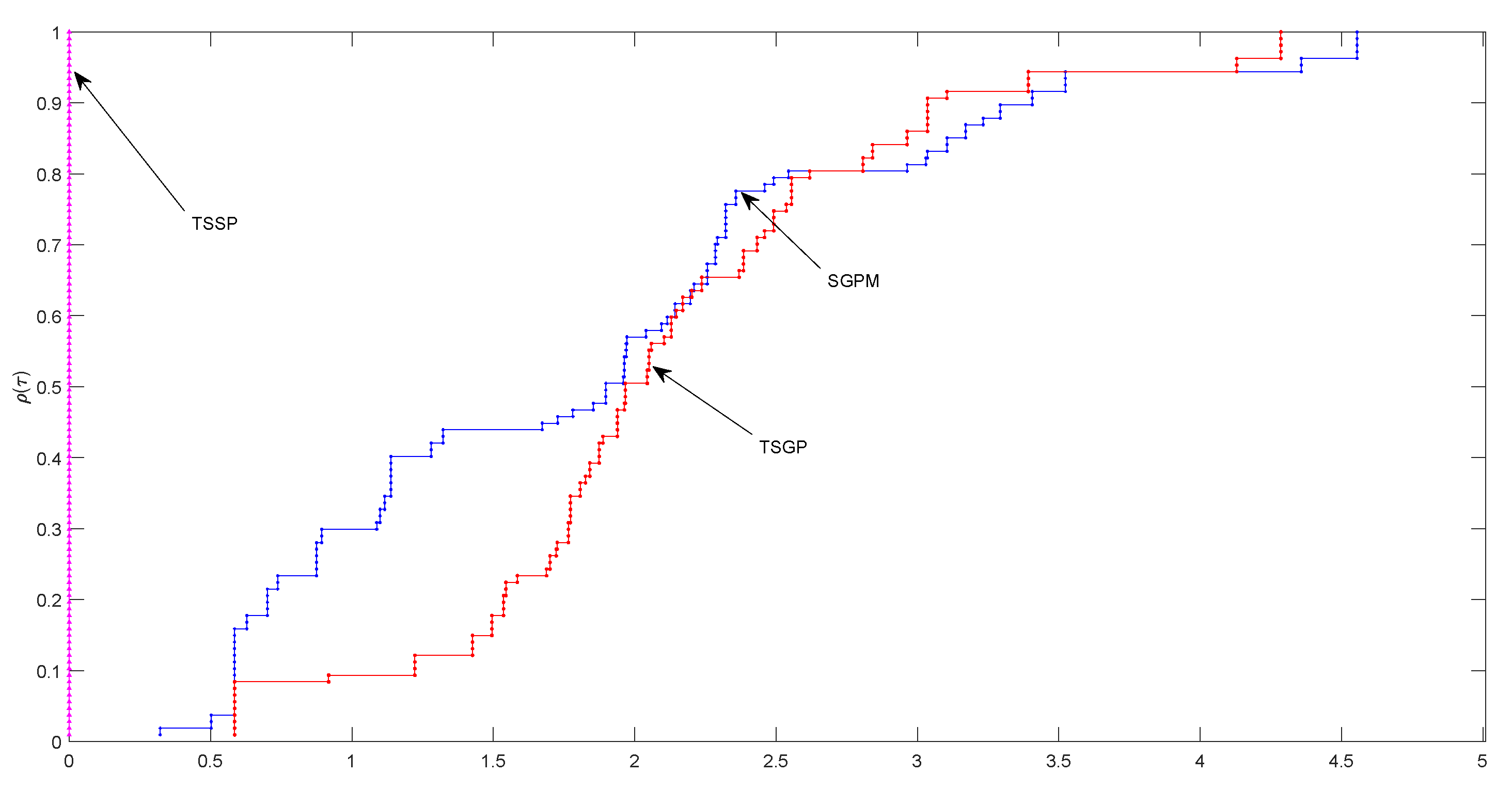
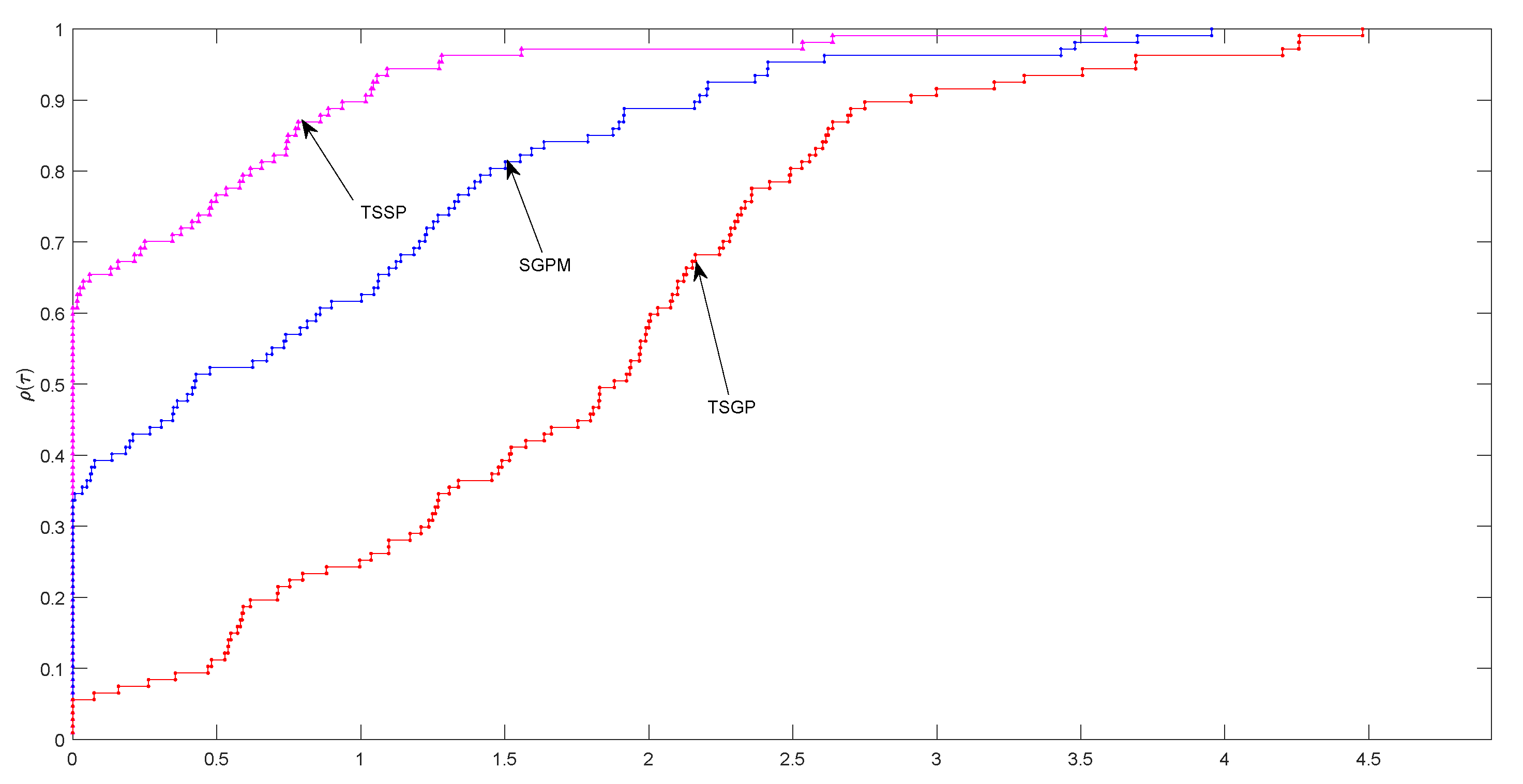
 Figure 1, Figure 2 and Figure 3 based on the Dolan and Mor e ´ performance profile [26]. This performance profile tells the percentage win by each solver. In all the experiments, we see from Figure 1, Figure 2 and Figure 3 that the proposed TSSP algorithm performs better with higher percentage win based on ITER, FVAL and TIME for solving all the test problems. In fact, the TSSP algorithm recorded 100 percent least FVAL for all the test problems.
We use the following test problems where F ( x ) = ( f 1 ( x ) , f 2 ( x ) , , f n ( x ) ) T , and x = ( x 1 , x 2 , , x n ) T .
Problem 1
([27]).
f 1 ( x ) = e x 1 1 f i ( x ) = e x i + x i 1 1 , i = 1 , 2 , , n 1 ,
where Λ = R + n .
Problem 2
([28]).
f i ( x i ) = log ( x i + 1 ) x i n , i = 1 , 2 , , n ,
where Λ = { x R n : i = 1 n x i n , x i > 1 , i = 1 , 2 , , n } .
Problem 3
([29]).
f i ( x ) = 2 x i sin | x i | , i = 1 , 2 , , n ,
where Λ = R + n .
Problem 4
([30]).
f i ( x ) = e x i 1 , i = 1 , 2 , , n ,
where Λ = R + n .
Problem 5
([29]).
f 1 ( x ) = x 1 e cos ( h ( x 1 + x 2 ) ) f i ( x ) = x i e cos ( h ( x i 1 + x i + x i + 1 ) ) , i = 1 , 2 , , n 1 , f n ( x ) = x n e cos ( h ( x n 1 + x n ) ) ,
where h = 1 n + 1 and Λ = R + n .
Problem 6
([31]).
f i ( x ) = x i sin ( | x i 1 | ) , i = 1 , 2 , , n 1 ,
where Λ = { x R n : i = 1 n x i n , x i 1 , i = 1 , 2 , , n } .

4. Applications in Image Deblurring

In this section, we apply the proposed Algorithm 1 to solve problems arising from compressive sensing, particularly image deblurring. Consider the following least square problem with 1 regularization term
min x 1 2 y E x 2 2 + μ x 1 ,
where x R n is the underlying images, y R k is the observed images, E R k × n ( k < < n ), linear operator, is an m × n blurring matrix, and the parameter μ > 0 . Problem (46) is of great importance because it appears in many areas of applications arising from compressive sensing. Recently, problem (46) has been investigated by many researchers and different kinds of iterative algorithms have been proposed in the literature [3,32,33,34,35]. Many algorithms for solving (46) fall into two categories namely: algorithms that required differentiability assumption and algorithms that are derivative free. Since 1 - norm is a nonsmooth function, algorithms that require the assumption of differentiabilty are not suitable for problem (46) in its original form. Consequently, either x 1 is approximated with some smooth function or problem (46) is reformulated into an equivalent problem. For instance, Figueiredo et al. [3] translate problem (46) into convex quadratic program as follows. For any x R n , we can find some vectors, say u , v R n such that
x = u v , u 0 , v 0 ,
where u i = max { 0 , x i } , v i = max { 0 , x i } for all i = 1 , 2 , , n . Thus, we can write x 1 = e n T ( u + v ) , where e n is an n - dimensional vector with all elements one. Therefore, we can rewrite problem (46) as
min u , v 1 2 y E ( u v ) 2 2 + μ e n T ( u + v ) . s . t u 0 , v 0
Furthermore, if we let q = [ u v ] T , then from Reference [3], we can write (47) as the following
min q 1 2 q T G q + c T q , s . t q 0 ,
where c = μ e 2 n + b b , b = E T y , G = E T E E T E E T E E T E . It is not difficult to see that G is a positive semi-definite matrix.
In Reference [36], the resulted constrained minimization problem (48) is further translated into the following linear variable inequality problem
Find q R n such that G q + c , q q 0 , q 0 .
Since the feasible region of q is R n , problem (49) is equivalent to the following linear complementary problem
Find q R n such that q 0 , G q + c 0 , G q + c , q = 0 .
We can see that the point q R n is a solution of the above linear complementary problem (50) if and only if it satisfies the following system of nonlinear equation
F ( q ) : = min { q , G q + c } = 0 .
The mapping F is a vector-valued and the “min” operator denotes the componentwise minimum of two vectors. Interestingly, Lemma 3 of Reference [37] and Lemma 2.2 of Reference [36] show that the mapping F satisfies Assumption 1 (ii) i.e., is Lipschitzian continuity and monotonicity. Therefore our proposed TSSP algorithm can be applied to solve it.

Image Deblurring Experiment

We tested the performance of the two-step TSSP algorithm in restoring some blurred images in comparison with the one-step spectral gradient method for 1 problems in compressed sensing (SGCS) [36]. The images used for the experiment are the well-known gray test images namely: Lena, House, Pepper, Camera man and Barbara where the size of each image is given in Table 5. The following metrics are used to assess the performance and quality of restoration by each algorithm tested: number of iteration (ITER), CPU time in seconds (TIME), signal-to-noise-ratio (SNR) which is defined as
SNR = 20 × log 10 x ¯ x x ¯ ,
and the structural similarity (SSIM) index that measure the similarity between the original image and the restored image [38] for each of the two experiments. The MATLAB implementation of the SSIM index can be obtained at http://www.cns.nyu.edu/~lcv/ssim/. To achieve fairness in comparison, each code was run from same initial point x 0 = E T y and terminate when
| f k f k 1 | | f k 1 | < 10 5 ,
where f k is the merit function evaluation at x k , with f ( x k ) = 1 2 y E x k 2 2 + μ x k 1 . The parameters used for both TSSP and SGCS in this experiment come from Reference [36] except for c = 1 in the line search (1) and α k = ( 0 . 999 k ) × ( 10 5 + F ( x 0 ) 2 ) .
The original, blurred and restored images by each algorithm are given in Figure 4. The two tested algorithms restored the blurred images successfully with different speed and level of quality. The results of the restoration by each algorithm are reported in Table 5. We see from Table 5 that TSSP restored all the five images with less ITER. Taking TIME into consideration, we see that though the SGCS is faster in restoring two of the images (i.e., Camera man and Barbara), TSSP is faster in restoring the remaining three images (i.e., Lena, House and Pepper). In addition, the SNR and SSIM values recorded by each algorithm revealed that TSSP restored the five blurred images with slightly better quality than SGCS except for Camera man. Taking everything together, this experiment shows that the two-step TSSP can deal with the 1 regularization problems effectively and can be a favourable alternative for image reconstruction.

5. Conclusions

This paper presents an efficient derivative-free iterative algorithm called TSSP for nonlinear monotone equations. It utilizes a two-step approach that incorporates the well-known BB parameters with a projection strategy. We showed that the TSSP converges globally under the Lipschitzian and monotonicity assumptions. Also, we proposed a new line search that is more general than the one proposed by Cheng in Reference [24], able to include the line search by Cheng as a special case. Preliminary numerical results reported in Table 2 shows that the parameter c introduced in the new line search defined by (1) may have some effect on the performance of the proposed algorithm. Numerical results presented revealed that the proposed TSSP algorithm has computational advantage and performs better than the two existing algorithms in References [17,25]. These results indicate that the two-step BB-like algorithm is superior to the existing one-step BB-like algorithms, especially on solving nonlinear equations. It is worth emphasizing that the TSSP algorithm improves existing results on monotone nonlinear equations. The results obtained in Section 3 show that the TSSP algorithm possessed excellent numerical performances with evidence of efficiently solving all the test problems considered with minimal number of iterations and function evaluations. The numerical results reported from the experiments of deblurring two-dimensional images from their limited measurements have shown that the two-step algorithm TSSP competes favorably with the one-step SGCS algorithm. Future work includes the extension of TSSP algorithm on different forms of optimization frameworks and applications such as nonlinear least-squares problems [39,40], neural networks [41,42] and machine learning [43,44].

Author Contributions

Conceptualization, L.W. and A.M.A.; methodology, A.M.A.; software, A.M.A. and H.M.; validation, A.M.A., L.W., P.K. and H.M.; formal analysis, A.M.A. and L.W.; investigation, A.M.A. and H.M.; resources, L.W. and P.K.; data curation, A.M.A. and H.M.; writing—original draft preparation, A.M.A.; writing—review and editing, A.M.A., L.W., P.K. and H.M.; visualization, P.K.; supervision, L.W. and P.K.; project administration, L.W. and P.K.; funding acquisition, P.K. and L.W. All authors have read and agreed to the published version of the manuscript.

Funding

The authors acknowledge the financial support provided by the Petchra Pra Jom Klao Doctoral Scholarship for Ph.D. program of King Mongkut’s University of Technology Thonburi (KMUTT) and Center of Excellence in Theoretical and Computational Science (TaCS-CoE), KMUTT. The first author was supported by the Petchra Pra Jom Klao Ph.D. Research Scholarship from King Mongkut’s University of Technology Thonburi (Contract No. 42/2560).

Acknowledgments

The authors would like to thank the anonymous referees for their useful comments. This project was supported by Center of Excellence in Theoretical and Computational Science (TaCS-CoE) Center under Computational and Applied Science for Smart Innovation research Cluster (CLASSIC), Faculty of Science, KMUTT. This work was done while the first author visits Yunnan University of Finance and Economics, Kunming China.

Conflicts of Interest

The authors declare no conflict of interest.

References

  1. Iusem, N.A.; Solodov, V.M. Newton-type methods with generalized distances for constrained optimization. Optimization 1997, 41, 257–278. [Google Scholar] [CrossRef]
  2. Zhao, Y.B.; Li, D. Monotonicity of fixed point and normal mappings associated with variational inequality and its application. SIAM J. Optim. 2001, 11, 962–973. [Google Scholar] [CrossRef]
  3. Figueiredo, M.A.T.; Nowak, R.D.; Wright, S.J. Gradient projection for sparse reconstruction: Application to compressed sensing and other inverse problems. IEEE J. Sel. Top. Signal Process. 2007, 1, 586–597. [Google Scholar] [CrossRef] [Green Version]
  4. Barzilai, J.; Borwein, J.M. Two-point step size gradient methods. IMA J. Numer. Anal. 1988, 8, 141–148. [Google Scholar] [CrossRef]
  5. Dai, Y.H.; Al-Baali, M.; Yang, X. A Positive Barzilai–Borwein-Like Stepsize and an Extension for Symmetric Linear Systems. Numer. Anal. Optim. 2015, 41, 59–75. [Google Scholar]
  6. Dai, Y.H.; Huang, Y.; Liu, X.W. A family of spectral gradient methods for optimization. Comput. Optim. Appl. 2019, 74, 43–65. [Google Scholar] [CrossRef] [Green Version]
  7. Birgin, E.G.; Martínez, J.M.; Raydan, M. Spectral projected gradient methods: Review and perspectives. J. Stat. Softw. 2014, 60, 1–21. [Google Scholar] [CrossRef]
  8. Fletcher, R. On the Barzilai-Borwein method. Optim. Control Appl. 2005, 60, 235–256. [Google Scholar]
  9. Dai, Y.H. A new analysis on the Barzilai-Borwein gradient method. J. Oper. Res. Soc. China 2013, 41, 187–198. [Google Scholar] [CrossRef] [Green Version]
  10. Dai, Y.H.; Kou, C. A Barzilai-Borwein conjugate gradient method. Sci. China Math. 2016, 59, 1511–1524. [Google Scholar] [CrossRef]
  11. Raydan, M. On the Barzilai and Borwein choice of steplength for the gradient method. IMA J. Numer. Anal. 1993, 13, 321–326. [Google Scholar] [CrossRef] [Green Version]
  12. Raydan, M. The Barzilai and Borwein gradient method for the large scale unconstrained minimization problem. SIAM J. Optim. 1997, 7, 26–33. [Google Scholar] [CrossRef]
  13. La Cruz, W.; Raydan, M. Nonmonotone spectral methods for large-scale nonlinear systems. Optim. Methods Softw. 2003, 18, 583–599. [Google Scholar] [CrossRef]
  14. La Cruz, W.; Martínez, J.M.; Raydan, M. Spectral residual method without gradient information for solving large-scale nonlinear systems of equations. Math. Comput. 2006, 75, 1429–1448. [Google Scholar] [CrossRef] [Green Version]
  15. Solodov, M.V.; Svaiter, B.F. A globally convergent inexact Newton method for systems of monotone equations. In Reformulation: Nonsmooth, Piecewise Smooth, Semismooth and Smoothing Methods; Springer: Boston, MA, USA, 1998; pp. 355–369. [Google Scholar]
  16. Zhang, L.; Zhou, W. Spectral gradient projection method for solving nonlinear monotone equations. J. Comput. Appl. Math. 2006, 96, 478–484. [Google Scholar] [CrossRef] [Green Version]
  17. Yu, Z.; Lin, J.; Sun, J.; Xiao, Y.; Liu, L.; Li, Z. Spectral gradient projection method for monotone nonlinear equations with convex constraints. Appl. Numer. Math. 2009, 59, 2416–2423. [Google Scholar] [CrossRef]
  18. Wang, C.; Wang, Y.; Xu, C. A projection method for a system of nonlinear monotone equations with convex constraints. Math. Methods Oper. Res. 2007, 66, 33–46. [Google Scholar] [CrossRef]
  19. Mohammad, H.; Abubakar, A.B. A positive spectral gradient-like method for large-scale nonlinear monotone equations. Bull. Comput. Appl. Math. 2017, 5, 97–113. [Google Scholar]
  20. Awwal, A.M.; Kumam, P.; Abubakar, A.B.; Wakili, A.; Pakkaranang, N. A New Hybrid Spectral Gradient Projection Method for Monotone System of Nonlinear Equations with Convex Constraints. Thai J. Math. 2018, 16, 125–147. [Google Scholar]
  21. Abubakar, A.B.; Kumam, P.; Mohammad, H. A note on the spectral gradient projection method for nonlinear monotone equations with applications. Comput. Appl. Math. 2020. [Google Scholar] [CrossRef]
  22. Mann, W.R. Mean value methods in iteration. Proc. Am. Math. Soc. 1953, 4, 506–510. [Google Scholar] [CrossRef]
  23. Ishikawa, S. Fixed points by a new iteration method. Proc. Am. Math. Soc. 1974, 44, 147–150. [Google Scholar] [CrossRef]
  24. Cheng, W. A PRP type method for systems of monotone equations. Math. Comput. Model. 2009, 50, 15–20. [Google Scholar] [CrossRef]
  25. Liu, J.; Duan, Y. Two spectral gradient projection methods for constrained equations and their linear convergence rate. J. Inequal. Appl. 2015, 1, 8. [Google Scholar] [CrossRef] [Green Version]
  26. Dolan, E.D.; Moré, J.J. Benchmarking optimization software with performance profiles. Math. Program. Ser. 2002, 91, 201–213. [Google Scholar] [CrossRef]
  27. La Cruz, W.; Martínez, J.M.; Raydan, M. Spectral Residual Method without Gradient Information for Solving Large-Scale Nonlinear Systems: Theory and Experiments; Technical Report RT-04-08; Universidad Central de Venezuela: Caracas, Venezuela, 2004; p. 37. Available online: http://kuainasi.ciens.ucv.ve/mraydan/download_papers/TechRep.pdf (accessed on 15 April 2020).
  28. Abubakar, A.B.; Kumam, P.; Mohammad, H.; Awwal, A.M. An Efficient Conjugate Gradient Method for Convex Constrained Monotone Nonlinear Equations with Applications. Mathematics 2019, 7, 767. [Google Scholar] [CrossRef] [Green Version]
  29. La Cruz, W. A spectral algorithm for large-scale systems of nonlinear monotone equations. Numer. Algorithms 2017, 76, 1109–1130. [Google Scholar] [CrossRef]
  30. Awwal, A.M.; Kumam, P.; Abubakar, A.B. A modified conjugate gradient method for monotone nonlinear equations with convex constraints. Appl. Numer. Math. 2019, 145, 507–520. [Google Scholar] [CrossRef]
  31. Yu, G.; Niu, S.; Ma, J. Multivariate spectral gradient projection method for nonlinear monotone equations with convex constraints. J. Ind. Manag. Optim. 2013, 9, 117–129. [Google Scholar] [CrossRef]
  32. Daubechies, I.; Defrise, M.; De Mol, C. An iterative thresholding algorithm for linear inverse problems with a sparsity constraint. Commun. Pure Appl. Math. A J. Issued Courant Inst. Math. Sci. 2004, 57, 1413–1457. [Google Scholar] [CrossRef] [Green Version]
  33. Hale, E.T.; Yin, W.; Zhang, Y. A Fixed-Point Continuation Method for ℓ1-Regularized Minimization with Applications to Compressed Sensing; CAAM TR07-07; Rice University: Houston, TX, USA, 2007; Volume 43. [Google Scholar]
  34. Beck, A.; Teboulle, M. A fast iterative shrinkage-thresholding algorithm for linear inverse problems. SIAM J. Imaging Sci. 2009, 2, 183–202. [Google Scholar] [CrossRef] [Green Version]
  35. Wright, S.J.; Nowak, R.D.; Figueiredo, M.A.T. Sparse reconstruction by separable approximation. IEEE Trans. Signal Process. 2009, 57, 2479–2493. [Google Scholar] [CrossRef] [Green Version]
  36. Xiao, Y.; Wang, Q.; Hu, Q. Non-smooth equations based methods for l1-norm problems with applications to compressed sensing. Nonlinear Anal. Theory Methods Appl. 2011, 74, 3570–3577. [Google Scholar] [CrossRef]
  37. Pang, J.S. Inexact Newton methods for the nonlinear complementarity problem. Math. Program. 1986, 36, 54–71. [Google Scholar] [CrossRef]
  38. Wang, Z.; Bovik, A.C.; Sheikh, H.R.; Simoncelli, E.P. Image quality assessment: From error visibility to structural similarity. IEEE Trans. Image Process. 2004, 13, 600–612. [Google Scholar] [CrossRef] [Green Version]
  39. Awwal, A.M.; Kumam, P.; Mohammad, H. Iterative algorithm with structured diagonal Hessian approximation for solving nonlinear least squares problems. arXiv 2020, arXiv:2002.01871. [Google Scholar]
  40. Mohammad, H.; Waziri, M.Y. Structured two-point stepsize gradient methods for nonlinear least squares. J. Optim. Theory Appl. 2019, 181, 298–317. [Google Scholar] [CrossRef] [Green Version]
  41. Li, G.; Zeng, Z. A neural-network algorithm for solving nonlinear equation systems. In Proceedings of the 2008 International Conference on Computational Intelligence and Security, Suzhou, China, 13–17 December 2008; Volume 1, pp. 20–23. [Google Scholar]
  42. Li, G.; Zeng, Z. A new neural network for solving nonlinear projection equations. Neural Netw. 2007, 20, 577–589. [Google Scholar]
  43. Zhu, Z.; Wang, H.; Zhang, B. A spectral conjugate gradient method for nonlinear inverse problems. Inverse Probl. Sci. Eng. 2018, 26, 1561–1589. [Google Scholar] [CrossRef]
  44. Bottou, L.; Cutis, F.E.; Nocedal, J. Optimization Methods for Large-Scale Machine Learning. SIAM Rev. 2018, 60, 223–311. [Google Scholar] [CrossRef]
Figure 1. Dolan and Mor e ´ performance profile with respect to number of iterations.
Symmetry 12 00874 g001
Figure 2. Dolan and Mor e ´ performance profile with respect to number of function evaluation.
Symmetry 12 00874 g002
Figure 3. Dolan and Mor e ´ performance profile with respect to CPU time.
Symmetry 12 00874 g003
Figure 4. The original images (first row), the blurred images (second row), the restored images by methods TSSP (third row) and SGCS (last row).
Symmetry 12 00874 g004
Table 1. Starting points used for the test problems.
Starting Points (SP)Values
x 1 ( 0.1 , 0.1 , 0.1 , , 0.1 ) T
x 2 ( 1 2 , 1 2 2 , 1 2 3 , , 1 2 n ) T
x 3 ( 2 , 2 , , 2 ) T
x 4 ( 1 , 1 2 , 1 3 , , 1 n ) T
x 5 ( 1 1 n , 1 2 n , 1 3 n , , 0 ) T
x 6 rand ( 0 , 1 )
Table 2. Numerical results showing the effect of the parameter c in the line search.
c12345
SPITERFVALNORMITERFVALNORMITERFVALNORMITERFVALNORMITERFVALNORM
P1 x 1 462.18 ×  10 7 462.18 ×  10 7 462.18 ×  10 7 462.18 ×  10 7 462.18 ×  10 7
x 2 792.82 ×  10 7 792.82 ×  10 7 792.82 ×  10 7 792.82 ×  10 7 792.82 ×  10 7
x 3 571.05 ×  10 7 571.05 ×  10 7 571.05 ×  10 7 571.05 ×  10 7 571.05 ×  10 7
x 4 796.34 ×  10 8 796.34 ×  10 8 796.34 ×  10 8 796.34 ×  10 8 796.34 ×  10 8
x 5 796.13 ×  10 8 796.13 ×  10 8 796.13 ×  10 8 796.13 ×  10 8 796.13 ×  10 8
x 6 792.77 ×  10 8 791.94 ×  10 8 792.3 ×  10 8 793.63 ×  10 8 791.94 ×  10 8
P2 x 1 352.41 ×  10 8 352.41 ×  10 8 352.41 ×  10 8 352.41 ×  10 8 352.41 ×  10 8
x 2 8105.09 ×  10 8 8105.09 ×  10 8 8105.09 ×  10 8 8105.09 ×  10 8 8105.09 ×  10 8
x 3 8101.23 ×  10 7 8101.23 ×  10 7 8101.23 ×  10 7 8101.23 ×  10 7 9111.49 ×  10 7
x 4 9111.53 ×  10 7 9111.53 ×  10 7 9111.53 ×  10 7 9111.53 ×  10 7 9111.53 ×  10 7
x 5 10125.81 ×  10 8 10125.81 ×  10 8 10125.81 ×  10 8 9113.45 ×  10 7 9113.45 ×  10 7
x 6 10124.97 ×  10 8 10126.04 ×  10 8 10125.27 ×  10 8 9113.51 ×  10 7 9113.49 ×  10 7
P3 x 1 354.03 ×  10 8 354.03 ×  10 8 354.03 ×  10 8 354.03 ×  10 8 354.03 ×  10 8
x 2 351.19 ×  10 7 351.19 ×  10 7 351.19 ×  10 7 351.19 ×  10 7 351.19 ×  10 7
x 3 468.27 ×  10 7 468.27 ×  10 7 468.27 ×  10 7 468.27 ×  10 7 468.27 ×  10 7
x 4 462.12 ×  10 8 462.12 ×  10 8 462.12 ×  10 8 462.12 ×  10 8 462.12 ×  10 8
x 5 571.46 ×  10 7 571.46 ×  10 7 571.46 ×  10 7 571.46 ×  10 7 571.46 ×  10 7
x 6 571.46 ×  10 7 571.44 ×  10 7 579.49 ×  10 8 571.37 ×  10 7 571.88 ×  10 7
P4 x 1 120120120120120
x 2 120120120120120
x 3 120120120120120
x 4 120120120120120
x 5 120120120120120
x 6 120120120120120
P5 x 1 357.96 ×  10 7 357.96 ×  10 7 357.96 ×  10 7 357.96 ×  10 7 357.96 ×  10 7
x 2 358.26 ×  10 7 358.26 ×  10 7 358.26 ×  10 7 358.26 ×  10 7 358.26 ×  10 7
x 3 352.18 ×  10 7 352.18 ×  10 7 352.18 ×  10 7 352.18 ×  10 7 352.18 ×  10 7
x 4 358.24 ×  10 7 358.24 ×  10 7 358.24 ×  10 7 358.24 ×  10 7 358.24 ×  10 7
x 5 356.8 ×  10 7 356.8 ×  10 7 356.8 ×  10 7 356.8 ×  10 7 356.8 ×  10 7
x 6 356.77 ×  10 7 356.81 ×  10 7 356.8 ×  10 7 356.79 ×  10 7 356.87 ×  10 7
P6 x 1 351.07 ×  10 7 351.07 ×  10 7 351.07 ×  10 7 351.07 ×  10 7 351.07 ×  10 7
x 2 9118.56 ×  10 9 9118.56 ×  10 9 8107.89 ×  10 7 8107.89 ×  10 7 8107.89 ×  10 7
x 3 461.15 ×  10 8 461.15 ×  10 8 461.15 ×  10 8 461.15 ×  10 8 461.15 ×  10 8
x 4 11131.26 ×  10 7 11131.26 ×  10 7 11131.26 ×  10 7 10128.08 ×  10 8 10128.08 ×  10 8
x 5 10129.99 ×  10 9 10129.99 ×  10 9 10129.99 ×  10 9 10129.99 ×  10 9 10129.99 ×  10 9
x 6 10122.72 ×  10 8 10121.67 ×  10 8 9111.46 ×  10 7 10122.84 ×  10 8 10123.82 ×  10 8
Table 3. Numerical results obtained by each solver.
TSSPSGPMTSGP
ProblemDIMSPITERFVALTIMENORMITERFVALTIMENORMITERFVALTIMENORM
P11000 x 1 460.234232.18 ×  10 7 5110.0714521.98 ×  10 7 10210.0274834.81 ×  10 7
x 2 790.0241292.82 ×  10 7 21430.0207058.07 ×  10 7 16330.009937.7 ×  10 7
x 3 570.004791.05 ×  10 7 8170.0054399.35 ×  10 9 14290.0066887.24 ×  10 7
x 4 790.0063486.34 ×  10 8 22450.0076466.66 ×  10 7 10210.0066828.79 ×  10 7
x 5 790.0071796.13 ×  10 8 7150.0055332.11 ×  10 8 8170.0079779.36 ×  10 7
x 6 790.010283.35 ×  10 8 7150.0085462.31 ×  10 8 14290.0061456.95 ×  10 7
50,000 x 1 460.0658636.63 ×  10 8 5110.066183.18 ×  10 7 11230.261788.02 ×  10 7
x 2 790.068252.82 ×  10 7 21430.168738.07 ×  10 7 16330.237247.7 ×  10 7
x 3 570.10917.38 ×  10 7 8170.0926836.61 ×  10 8 16330.198287.44 ×  10 7
x 4 790.078156.35 ×  10 8 22450.195876.67 ×  10 7 10210.117778.72 ×  10 7
x 5 8100.0908368 ×  10 9 7150.0528031.34 ×  10 7 17350.2127.38 ×  10 7
x 6 8100.0819646.53 ×  10 9 7150.0490611.32 ×  10 7 16330.174288.9 ×  10 7
100,000 x 1 460.105877.46 ×  10 8 5110.122334.34 ×  10 7 12250.356984.49 ×  10 7
x 2 790.139382.82 ×  10 7 21430.366698.07 ×  10 7 16330.533827.7 ×  10 7
x 3 680.172025.19 ×  10 9 8170.154269.34 ×  10 8 17350.589494.19 ×  10 7
x 4 790.152236.35 ×  10 8 22450.4736.67 ×  10 7 10210.249478.72 ×  10 7
x 5 8100.220731.13 ×  10 8 7150.10361.9 ×  10 7 18370.460194.18 ×  10 7
x 6 8100.155841.18 ×  10 8 7150.10351.94 ×  10 7 17350.512777.07 ×  10 7
P21000 x 1 350.0536922.41 ×  10 8 19390.0220916.53 ×  10 7 14290.0092739.17 ×  10 7
x 2 8100.0062475.09 ×  10 8 19390.0083775.84 ×  10 7 14290.010227.19 ×  10 7
x 3 8100.0070911.23 ×  10 7 24490.0091187.53 ×  10 7 19390.01715.49 ×  10 7
x 4 9110.0069621.53 ×  10 7 20410.007657.01 ×  10 7 15310.0117347.44 ×  10 7
x 5 10120.0100535.81 ×  10 8 23470.0103989.51 ×  10 7 17350.0120629.65 ×  10 7
x 6 10120.007337.06 ×  10 8 23470.0096599.64 ×  10 7 17350.0150279.61 ×  10 7
50,000 x 1 350.0587321.71 ×  10 7 22450.270951.14 ×  10 8 17350.262774.05 ×  10 7
x 2 8100.11125.09 ×  10 8 19390.171435.86 ×  10 7 14290.25047.22 ×  10 7
x 3 8100.111578.68 ×  10 7 27550.336451.35 ×  10 8 21430.442856.23 ×  10 7
x 4 9110.112861.52 ×  10 7 20410.187587.05 ×  10 7 15310.268277.49 ×  10 7
x 5 10120.137384.2 ×  10 7 26530.249058.68 ×  10 7 20410.323684.36 ×  10 7
x 6 10120.156184.3 ×  10 7 26530.366058.69 ×  10 7 20410.311564.35 ×  10 7
100,000 x 1 350.0912772.42 ×  10 7 21430.412743.2 ×  10 8 17350.554815.73 ×  10 7
x 2 8100.195255.09 ×  10 8 19390.350455.86 ×  10 7 14290.483087.22 ×  10 7
x 3 9110.276311.21 ×  10 8 27550.6281.91 ×  10 8 21430.665148.81 ×  10 7
x 4 9110.327551.52 ×  10 7 20410.440647.05 ×  10 7 15310.486987.49 ×  10 7
x 5 10120.259095.94 ×  10 7 27550.540566.2 ×  10 7 20410.744116.16 ×  10 7
x 6 10120.289415.64 ×  10 7 27550.579846.19 ×  10 7 20410.669266.16 ×  10 7
P31000 x 1 350.0275054.03 ×  10 8 5110.0044181.97 ×  10 8 11230.0049324.32 ×  10 7
x 2 350.0022431.19 ×  10 7 5110.0048813.84 ×  10 8 8170.0061485.84 ×  10 7
x 3 460.0039018.27 ×  10 7 6130.003284.62 ×  10 7 13270.0102016.63 ×  10 7
x 4 460.0029992.12 ×  10 8 5110.0022163.93 ×  10 7 11230.0078599.11 ×  10 7
x 5 570.0041831.46 ×  10 7 6130.0023054.67 ×  10 8 14290.0092218.68 ×  10 7
x 6 570.0025171.08 ×  10 7 6130.0026344.62 ×  10 8 14290.0079648.55 ×  10 7
50,000 x 1 350.0378392.85 ×  10 7 5110.0468131.39 ×  10 7 13270.30244.88 ×  10 7
x 2 350.0437021.19 ×  10 7 5110.0755473.84 ×  10 8 8170.135.84 ×  10 7
x 3 570.0676545.79 ×  10 8 7150.0532263.24 ×  10 8 15310.20877.48 ×  10 7
x 4 460.0434132.13 ×  10 8 5110.0416883.93 ×  10 7 11230.202569.12 ×  10 7
x 5 680.057191.03 ×  10 8 6130.0521963.31 ×  10 7 16330.319849.81 ×  10 7
x 6 680.0800351.01 ×  10 8 6130.0476763.31 ×  10 7 16330.310029.75 ×  10 7
100,000 x 1 350.0749484.03 ×  10 7 5110.0955031.97 ×  10 7 13270.384016.89 ×  10 7
x 2 350.0680171.19 ×  10 7 5110.0709573.84 ×  10 8 8170.189475.84 ×  10 7
x 3 570.261138.19 ×  10 8 7150.136524.58 ×  10 8 16330.517684.22 ×  10 7
x 4 460.136682.13 ×  10 8 5110.0739033.93 ×  10 7 11230.316749.12 ×  10 7
x 5 680.165271.46 ×  10 8 6130.0805724.68 ×  10 7 17350.465765.54 ×  10 7
x 6 680.154691.5 ×  10 8 6130.10354.68 ×  10 7 17350.490755.52 ×  10 7
Table 4. Numerical results obtained by each solver.
TSSPSGPMTSGP
ProblemDIMSPITERFVALTIMENORMITERFVALTIMENORMITERFVALTIMENORM
P41000 x 1 120.0249990130.0020820130.0026650
x 2 120.001530130.001492010210.0137086.89 ×  10 7
x 3 120.0020330130.0017520130.0030470
x 4 120.001605011230.004168.04 ×  10 7 130.0012040
x 5 120.001898020410.0069666.33 ×  10 7 17350.0245135.22 ×  10 7
x 6 120.002199020410.0050646.89 ×  10 7 17350.0095685.82 ×  10 7
50,000 x 1 120.0098160130.021620130.0275670
x 2 120.0157920130.010298010210.116976.89 ×  10 7
x 3 120.0195390130.0096520130.049430
x 4 120.022933011230.0875667.32 ×  10 7 130.0164330
x 5 120.014115023470.152245.8 ×  10 7 19390.259565.87 ×  10 7
x 6 120.015431023470.172125.81 ×  10 7 19390.343965.8 ×  10 7
100,000 x 1 120.0293330130.0180750130.0271670
x 2 120.0295020130.021229010210.209626.89 ×  10 7
x 3 120.0294130130.0291060130.0425740
x 4 120.029978011230.157857.32 ×  10 7 130.0296470
x 5 120.024201023470.375038.2 ×  10 7 19390.462688.31 ×  10 7
x 6 120.023344023470.302688.28 ×  10 7 19390.446898.24 ×  10 7
P51000 x 1 350.0265847.96 × 10 7 22450.0127814.76 × 10 7 20410.023548.85 × 10 7
x 2 350.0035138.26 × 10 7 21430.0214469.78 × 10 7 20410.0264189.18 × 10 7
x 3 350.0031162.18 × 10 7 20410.0116015.12 × 10 7 19390.020136.08 × 10 7
x 4 350.0029868.24 × 10 7 24490.0084551.26 × 10 7 20410.0385479.16 × 10 7
x 5 350.0033866.8 × 10 7 26530.0151252.64 × 10 8 20410.0210847.56 × 10 7
x 6 350.0032386.8 × 10 7 26530.0148892.67 × 10 8 20410.0193517.56 × 10 7
50,000 x 1 680.108417.24 × 10 7 18370.281111.99 × 10 8 22450.638379.98 × 10 7
x 2 680.120087.52 × 10 7 19390.352525.32 × 10 7 23470.590834.14 × 10 7
x 3 460.0918087.79 × 10 7 17350.244945.52 × 10 7 21430.617626.85 × 10 7
x 4 680.103567.52 × 10 7 19390.261991.04 × 10 8 23470.582764.14 × 10 7
x 5 680.11186.19 × 10 7 22450.420865.64 × 10 8 22450.688668.53 × 10 7
x 6 680.130426.19 × 10 7 20410.304572.21 × 10 7 22450.571088.53 × 10 7
100,000 x 1 790.39915.17 × 10 7 17350.532295.58 × 10 8 23471.41835.64 × 10 7
x 2 790.330165.37 × 10 7 19390.706427.53 × 10 7 23471.29365.85 × 10 7
x 3 570.224235.57 × 10 7 17350.539797.8 × 10 7 21431.07289.69 × 10 7
x 4 790.319265.37 × 10 7 18370.594932.92 × 10 8 23471.34595.85 × 10 7
x 5 680.253848.75 × 10 7 19390.693541.21 × 10 8 23471.26824.82 × 10 7
x 6 680.371718.75 × 10 7 20410.620583.13 × 10 7 23471.30074.82 × 10 7
P61000 x 1 350.0109551.07 × 10 7 23470.012576.93 × 10 7 19390.0159194.69 × 10 7
x 2 9110.0068.56 × 10 9 23470.0123849.68 × 10 7 19390.017165.74 × 10 7
x 3 460.0064741.15 × 10 8 6130.0021992.21 × 10 7 13270.0094288.36 × 10 7
x 4 11130.0085021.26 × 10 7 23470.0135569.78 × 10 7 19390.0127285.69 × 10 7
x 5 10120.0101029.99 × 10 9 7150.0041832.36 × 10 7 19390.0100114.42 × 10 7
x 6 10120.0070117.27 × 10 9 7150.0068912.93 × 10 7 19390.0095424.06 × 10 7
50,000 x 1 350.0612557.6 × 10 7 24490.230972.6 × 10 8 21430.327755.28 × 10 7
x 2 11130.135652.66 × 10 7 25510.238411.83 × 10 8 21430.343166.46 × 10 7
x 3 460.0624628.1 × 10 8 7150.0658558.32 × 10 9 15310.255299.4 × 10 7
x 4 14160.204461.62 × 10 8 26530.260128.69 × 10 7 21430.313486.46 × 10 7
x 5 10120.146577.62 × 10 8 8170.0711418.94 × 10 9 21430.346695.05 × 10 7
x 6 10120.155977.06 × 10 8 8170.0912298.84 × 10 9 21430.356755.27 × 10 7
100,000 x 1 460.111845.71 × 10 9 24490.577693.68 × 10 8 21430.627647.47 × 10 7
x 2 14160.441771.79 × 10 7 25510.451882.59 × 10 8 21430.64279.14 × 10 7
x 3 460.203051.15 × 10 7 7150.140391.18 × 10 8 16330.516875.3 × 10 7
x 4 14160.306291.42 × 10 7 27550.494756.18 × 10 7 21430.655039.14 × 10 7
x 5 9110.189472.07 × 10 8 8170.134161.26 × 10 8 21430.676697.15 × 10 7
x 6 9110.252672.25 × 10 8 8170.160381.25 × 10 8 21430.678867.17 × 10 7
Table 5. Test results for TSSP and SGCS in image restoration.
TSSPSGCS
ImageSizeITERTIME(s)SNRSSIMITERTIME(s)SNRSSIM
Lena256 × 2561138.8424.250.9021811.0923.700.90
House256 × 25612116.5322.860.8723517.4723.610.87
Pepper256 × 2561008.6927.580.8916712.0527.020.89
Camera man256 × 256212.2020.330.84282.1920.560.84
Barbara512 × 5122212.6919.160.762311.0819.160.76

