Switching Perfect Control Algorithm

Abstract

The application of the switching control framework to the perfect control algorithm is presented in this paper. Employing the nonunique matrix inverses, the different closed-loop properties are obtained and further enhanced with possible switching methodology implementation. Simulation examples performed in the MATLAB/Simulink environment clearly show that the new framework can lead to benefits in terms of the control energy, speed, and robustness of the perfect control law. The possibility of transferring the new obtained results to the symmetrical nonlinear plants seems to be immediate.

1. Introduction

The design of multivariable control systems has always been considered as a complex problem in modern control theory. Throughout the years, numerous instances were developed with the aim of minimizing different performance indices. Naturally, differentiators such as control error, energy, or speed were used as clear assessment factors allowing for numerical comparison of various control structures. The pursuit of other desired properties led to clarification of such strategies as optimal, adaptive, energy efficient, or deadbeat control algorithms [1,2,3,4,5,6], whilst the minimization of control error has resulted in the development of the perfect control algorithm [7,8].

The perfect control law is one of the most energy-demanding scenario, which ensures that the control error disappears right after delay time deriving from the system description [9]. The perfect law is a member of the Inverse Model Control (IMC) family; thus, at some point of the closed-loop system design process, a kind of inverse is used. It is worth mentioning that in the case of nonsquare systems, i.e., systems with different numbers of inputs and outputs, the inverse task has various nonunique solutions entailing different control properties [10].

The matter of obtaining the inverse of nonsquare matrices is yet another wide scope of research topics considered in this paper. For years, the unique minimum-norm right T-inverse has been used in different inverse applications due to its said minimum-energy property [11,12]. However, it has also been shown that in the perfect or minimum-variance control instance, the uniqueness can be a drawback. Since for the non-minimum-phase systems, the perfect control poles can be unstable, the need to acknowledge some nonunique solutions has grown remarkably [13]. Naturally, the nonunique inverses turned out to be a remedy for all of the mentioned disadvantages. With the application of the so-called degrees of freedom, almost an infinite number of possible solutions could be employed in different control strategies [14], including the perfect control design. Properties connected with minimum energy or maximum speed were established using, e.g., the arbitrary $\sigma$- or H-inverse [15,16].

Interestingly, the idea of having different sets of the closed-loop properties obtained in a single control task is not a new one. For example, the switching systems or sliding mode controllers have already been developed with a plethora of possible applications [14,17,18,19]. With time-varying controller parameters, the possibility to influence the closed-loop system intentionally was given to the control designer.

Based on the above, it can be inferred that merging the mentioned strategies seems to be a very interesting, yet unexplored area of the control field. Having both nonunique inverses and sliding mode frameworks, the possibility to influence both transient and steady-states of perfect control arbitrarily has just now been invented. This paper constitutes the first approach to obtain the described hybrid control system with the goal to obtain a possibly accurate and fast perfect control algorithm with reasonable energy expenditure. The main achievement of the manuscript in the form of the switching perfect control law derived from the generalized inverse application provides the proper basis for further research investigation. The union of the above-mentioned techniques should finally lead to the re-confirmation of the sliding mode control approach strictly dedicated to the non-stationary state-space linear multivariable plants.

Thus, this paper is organized as follows. At the beginning, the system description is given. Based on the state and output equations, the perfect control algorithm is described in the third section. In Section 4, different inverses dedicated to nonsquare matrices are discussed together with their possible application in regard to perfect control. The main focus of this paper is considered in Section 5; a switching perfect-based control algorithm is developed here. The simulation study performed in Section 6 shows the innovative behavior obtained with the application of switching perfect state feedback. Naturally, the conclusions are given at the end of the paper.

2. System Description

The main focus of the presented work is a study covering multivariable systems. Specifically, cases covering nonsquare systems, i.e., plants with different numbers of input and output variables, are considered. Thus, a state-space framework in the following form:

$$\begin{array}{cc}\hfill \mathbf{x}(k+1)& =\mathbf{A}\mathbf{x}\left(k\right)+\mathbf{B}\mathbf{u}\left(k\right),\mathbf{x}\left(0\right)={\mathbf{x}}_0,\hfill \\ \hfill \mathbf{y}\left(k\right)& =\mathbf{C}\mathbf{x}\left(k\right),\hfill \end{array}$$

(1)

is selected to describe the system being subject to the control actions. To be exact, we also specify the dimensions of the parameter matrices to be $\mathbf{A}\in {\Re }^{n\times n}$, $\mathbf{B}\in {\Re }^{n\times n_u}$, $\mathbf{C}\in {\Re }^{n_y\times n}$. Additionally, $\mathbf{x}\left(k\right)$, $\mathbf{u}\left(k\right)$, and $\mathbf{y}\left(k\right)$ are the n-state, $n_u$-input, and $n_y$-output vectors, respectively, whereas the initial state is denoted by ${\mathbf{x}}_0$. Moreover, for the requirements of perfect control, we are assuming that the system is controllable and that the matrix product $\mathbf{CB}$ is right-invertible [8].

3. Perfect Control

The perfect control algorithm is usually obtained for Linear Time-Invariant (LTI) systems using a d-step output predictor, in general. However, in the case of plants with single unit delay in the state description, it is obtained by equating the one-step deterministic output predictor $\mathbf{y}(k+1)=\mathbf{C}\left(\mathbf{x}\right(k+1\left)\right)=\mathbf{CBu}\left(k\right)+\mathbf{CAx}\left(k\right)$ to the reference/setpoint ${\mathbf{y}}_{\mathrm{ref}}$. With proper transition, the perfect control law is obtained in the following form:

$$\mathbf{u}\left(k\right)={\left(\mathbf{C}\mathbf{B}\right)}^{\mathrm{R}}({\mathbf{y}}_{\mathrm{ref}}\left(k\right)-\mathbf{C}\mathbf{A}\mathbf{x}\left(k\right)),$$

(2)

where (${\mathbf{CB})}^{\mathrm{R}}$ denotes any right inverse of $\mathbf{CB}$.

Remark 1.

Naturally, the right inverse of the $\mathbf{CB}$ matrix used in the perfect control law can be obtained in different numeric procedures described, e.g., in [12,16,20].

With the application of the perfect control formula, the closed-loop system can be described in terms of the state-feedback framework as follows:

$$\mathbf{u}\left(k\right)=-\mathbf{K}\mathbf{x}\left(k\right)+\mathbf{B}\mathbf{v}\left(k\right),$$

(3)

where $\mathbf{K}={\left(\mathbf{C}\mathbf{B}\right)}^{\mathrm{R}}\mathbf{C}\mathbf{A}$ and $\mathbf{v}\left(k\right)$ denotes new arbitrary input signal. However, according to the state-space framework from Equation (1), we can write the closed-loop state equation as follows:

$$\mathbf{x}(k+1)=(\mathbf{A}-\mathbf{BK})\mathbf{x}\left(k\right)+\mathbf{B}{\left(\mathbf{CB}\right)}^{\mathrm{R}}\mathbf{v}\left(k\right).$$

(4)

Of course, for such a given state equation, the output $\mathbf{y}\left(k\right)=\mathbf{C}\mathbf{x}\left(k\right)$ with reference/setpoint $\mathbf{B}\mathbf{v}\left(k\right)=\mathbf{B}{\left(\mathbf{CB}\right)}^{\mathrm{R}}{\mathbf{y}}_{\mathrm{ref}}\left(k\right)$, the output formula can be reduced to the following statement:

$$\mathbf{y}(k+1)={\mathbf{y}}_{\mathrm{ref}}\left(k\right).$$

(5)

Naturally, in such a case, the control error will assume the lowest possible value. Interestingly, this behavior is obtained in every case; thus, the Bounded-Input, Bounded-Output (BIBO) stability shall not be considered in the perfect control analysis. Of course, the Bounded-Input, Bounded-State (BIBS) stability of such a system depends on the closed-loop perfect control plant poles, which are the solution of the characteristic equation as follows:

$$det(z\mathbf{I}-\mathbf{A}+\mathbf{B}\mathbf{K})=0.$$

(6)

Aiming for the further clarity of the notion, we will introduce the closed-loop system matrix ${\mathbf{A}}^{\ast }$. Now, the perfect control stability can be calculated according to the formula employing the closed-loop system matrix as follows:

$$det(z\mathbf{I}-{\mathbf{A}}^{\ast })=0.$$

(7)

The stability, the same as other closed-loop properties, can be assigned with the usage of different state-feedback gains. Moreover, in the perfect control strategy developed for a nonsquare plant, there is a wide possibility to obtain numerous solutions using nonunique inverses. Thus, the foundations of nonunique inverse calculation are given in the next section.

4. Nonsquare Matrix Inverses

The idea of inverse matrix calculation is a mathematical concept frequently used in control applications. The whole branch of the so-called inverse model control algorithms is based on some kind of parameter or matrix inverses. Through various arrangements, the minimum-norm Moore–Penrose, approach has mainly been used due to its established properties connected with energy performance. The mentioned minimum-norm, later recalled as the right T-inverse, of given right-invertible matrix $\mathbf{M}$ is in the following form:

$${\mathbf{M}}_0^{\mathrm{R}}={\mathbf{M}}^{\mathrm{T}}{\left(\mathbf{M}{\mathbf{M}}^{\mathrm{T}}\right)}^{-1}.$$

(8)

The unique approach consisting of the T-inverse is often used as a benchmark for other, nonunique inverse techniques. This nonuniqueness can help to eliminate the drawbacks inherent to a unique numerical solution. Various properties of IMC schemes have been assigned in the past with the application of, e.g., the nonunique right $\sigma$-inverse. The mentioned inverse can be obtained with the following equation:

$${\mathbf{M}}_{\sigma }^{\mathrm{R}}={\beta }^{\mathrm{T}}{\left(\mathbf{M}{\beta }^T\right)}^{-1},$$

(9)

where matrix $\beta$ is the so-called degree of freedom. With a properly executed process of determining the numerical values of $\beta$, there is a possibility to assign almost arbitrarily the desired closed-loop perfect control behavior. It was already shown that employment of the right $\sigma$-inverse can be beneficial in terms of pole placement, control energy, or robustness. Of course, similar properties can be obtained with the application of any nonsquare inverse. Nevertheless, it seems interesting for it to be the Singular Value Decomposition (SVD)-based right H-inverse. Based on the SVD procedure, any matrix $\mathbf{M}$ can be rewritten in the following form:

$$\mathbf{M}=\mathbf{U}\Sigma {\mathbf{V}}^{\mathrm{T}},$$

(10)

where $\Sigma =\left[\begin{array}{c}\mathsf{\Lambda }\mathbf{0}\end{array}\right]$, with $\mathsf{\Lambda }$ revealing the eigenvalues of $\mathbf{M}$.

Remark 2.

Matrix Λ in the case of nonsingular $\mathbf{M}$ is just a diagonal matrix with eigenvalues on the main diagonal. In any more complex scenarios, the Λ matrix shall assume a so-called Jordan form, which is a certain type of extension of the diagonalization process.

The right inverse of matrix $\mathbf{M}$ is obtained by calculating the following expression:

$${\Sigma }^{\mathrm{R}}=\left[\begin{array}{c}{\mathsf{\Lambda }}^{-1}\\ \mathbf{L}\end{array}\right],$$

(11)

where $\mathbf{L}$ is the H-inverse-related matrix being the degree of freedom. The final H-inverse form is obtained directly with the equation presented below:

$${\mathbf{M}}_H^{\mathrm{R}}={\left({\mathbf{V}}^{\mathrm{T}}\right)}^{-1}{\Sigma }^{\mathrm{R}}{\mathbf{U}}^{-1}.$$

(12)

Having three different ways of appointing the right inverse of a nonsquare matrix, let us now continue with the application of nonunique inverses in perfect control scenarios. Significantly, the particular approach covering the time-varying solution of the matrix inverse problem is presented in the next section.

5. Switching Perfect Control

During the perfect control design, the selection of the degrees of freedom has a major influence on determining the closed-loop properties. With almost an infinite number of possible outcomes, some numeric procedures were developed to determine the “good” sets of the degrees of freedom. However, the classical approach has considered only the parameter degrees of freedom, but this limitation was maintained only for computational reasons. Now, with the advancement in computational power, those limitations are no longer necessary to impose. The first attempts covering varying state feedback were already undertaken, providing valuable foundations for further studies. Naturally, the changing parameters can be understood in different manners. Of course, the degree of freedom $\beta$ or L can be in the form of a polynomial matrix resulting in time-varying state feedback, entailing the whole closed-loop plant to be a Linear Time-Varying (LTV) one [21,22]. On the other hand, in the perfect control scenario, there is the possibility to change one perfect feedback gain to another without loss of perfect output behavior. In such a case, the classical perfect control law with the distinction of two $\mathbf{CB}$ inverses that can be described by the following equation:

$$\mathbf{u}\left(k\right)={\left(\mathbf{C}\mathbf{B}\right)}^{\mathrm{R}}{\mathbf{y}}_{\mathrm{ref}}\left(k\right)-{\left(\mathbf{C}\mathbf{B}\right)}^{\mathrm{R}}\mathbf{C}\mathbf{A}\mathbf{x}\left(k\right),$$

(13)

can also be developed with the admission of a nonunique inverse solution. Henceforth, the inverses involved in the perfect control design will now be considered twofold, depending on the switching time. The application of such switching control can be described as follows:

$$\mathbf{u}\left(k\right)={\left(\mathbf{C}\mathbf{B}\right)}^{\mathrm{R}}\left(k\right){\mathbf{y}}_{\mathrm{ref}}\left(k\right)-{\left(\mathbf{C}\mathbf{B}\right)}^{\mathrm{R}}\left(k\right)\mathbf{C}\mathbf{A}\mathbf{x}\left(k\right).$$

(14)

Of course, the switching inverse can be understood as twofold. The first approach in terms of perfect state feedback changing after some threshold time $k_s$ is as below:

$${\mathbf{CB}}^{\mathrm{R}}\left(k\right)=\begin{array}{c}{\mathbf{CB}}_1^{\mathrm{R}}fork\le k_s,\hfill \\ {\mathbf{CB}}_2^{\mathrm{R}}fork>k_s.\hfill \end{array}$$

(15)

It is rather clear that with such perfect control gains, all the closed-loop system properties will also change. To cover the changes of Equation (15), the perfect control closed-loop system matrix will also be dependent on the switched parameter matrix in the following manner:

$$\mathbf{A}-\mathbf{BK}\left(k\right)=\begin{array}{c}\mathbf{A}-{\mathbf{BK}}_{1}fork\le k_s\hfill \\ \mathbf{A}-{\mathbf{BK}}_{2}fork>k_s.\hfill \end{array}$$

(16)

Of course, the changing parameters inside the closed-loop system will result in different time-varying behaviors. The transition between subsequent internal states of the control plant can naturally be described in the following manner:

$$\mathbf{x}(k+1)={\mathbf{A}}^{\ast }\left(k\right)\mathbf{x}\left(k\right).$$

(17)

The LTV matrix ${\mathbf{A}}^{\ast }\left(k\right)$ will of course influence the transient states of control system response. With switching dynamics, the various schemes of perfect control can be obtained. The generalized form involves a number of possible switching procedures. However, in this particular study, the state feedback is switched only once. The reasoning for that is the aim of the possibly clear notion in further formulas.

Remark 3.

The equation presented above can also be used for the classical time-invariant framework with substitution ${\mathbf{A}}^{\ast }\left(k\right)={\mathbf{A}}^{\ast }$. It is worth mentioning that the time-varying part is expected to have greater influence in the close surroundings of switching time.

Of course, the stability of such a system is yet another complex issue. Naturally, this property can be described by the evolutionary operator in the following form [21]:

$$\varphi (k,i)={\mathbf{A}}^{\ast }\left(k\right){\mathbf{A}}^{\ast }(k-1)\dots {\mathbf{A}}^{\ast }(k-i),$$

(18)

that was originally introduced to describe the time-varying systems. Moreover, in the former case, the stability has been related to the following relation:

$$\left|\right|\varphi (k,i)\left|\right|\le M{e}^{-\gamma (k-i)},$$

(19)

for some positive M, $\gamma$, and $k\ge i$. This can be understood as that the state variables vary towards some finite state in a finite time. Thus, the above definition covers the BIBO stability of the linear state-space system. Additionally, in the considered case of single switching action, the stability can be determined based on the eigenvalues of the pre- and post-switching closed-loop system matrix. Additionally, the stability of transition between the two mentioned states shall be acknowledged with the use of an evolutionary operator mentioned above.

On the other hand, for systems with nonzero reference values, there is an additional possibility to influence the control plant. The pre-amplifier of reference value contained in ${\left(\mathbf{C}\mathbf{B}\right)}^{\mathrm{R}}\left(k\right){\mathbf{y}}_{\mathrm{ref}}\left(k\right)$ can again be switched during simulation time. Similarly to the switching state feedback, the switching pre-amplifier can be described with the following relations:

$${\left(\mathbf{C}\mathbf{B}\right)}^{\mathrm{R}}\left(k\right){\mathbf{y}}_{\mathrm{ref}}\left(k\right)=\begin{array}{c}{\left(\mathbf{C}\mathbf{B}\right)}_1^{\mathrm{R}}{\mathbf{y}}_{\mathrm{ref}}\left(k\right)fork\le k_s\hfill \\ {\left(\mathbf{C}\mathbf{B}\right)}_2^{\mathrm{R}}{\mathbf{y}}_{\mathrm{ref}}\left(k\right)fork>k_s.\hfill \end{array}$$

(20)

Thus, in the switching perfect control design process, along with the nonunique inverses with included degrees of freedom, there are other parameters that can be changed in order to obtain a different system response. Said additional degrees of freedom will be the already mentioned switching times of both the state feedback and setpoint pre-amplifier. Of course, having so much potential to influence the perfect control system, there is a need to pick some sets of “good” and “bad” solutions for a given plant carefully. Alongside such performance indices as the control energy, speed, or amplitude of the signals fed into the plant, the main differentiator will still be the already mentioned stability of the closed-loop perfect control systems. Naturally, the basis of the switching inverse model control is strictly derived from the classical perfect control scenario with established output run on the reference value after time delay accompanying the state-space plant description.

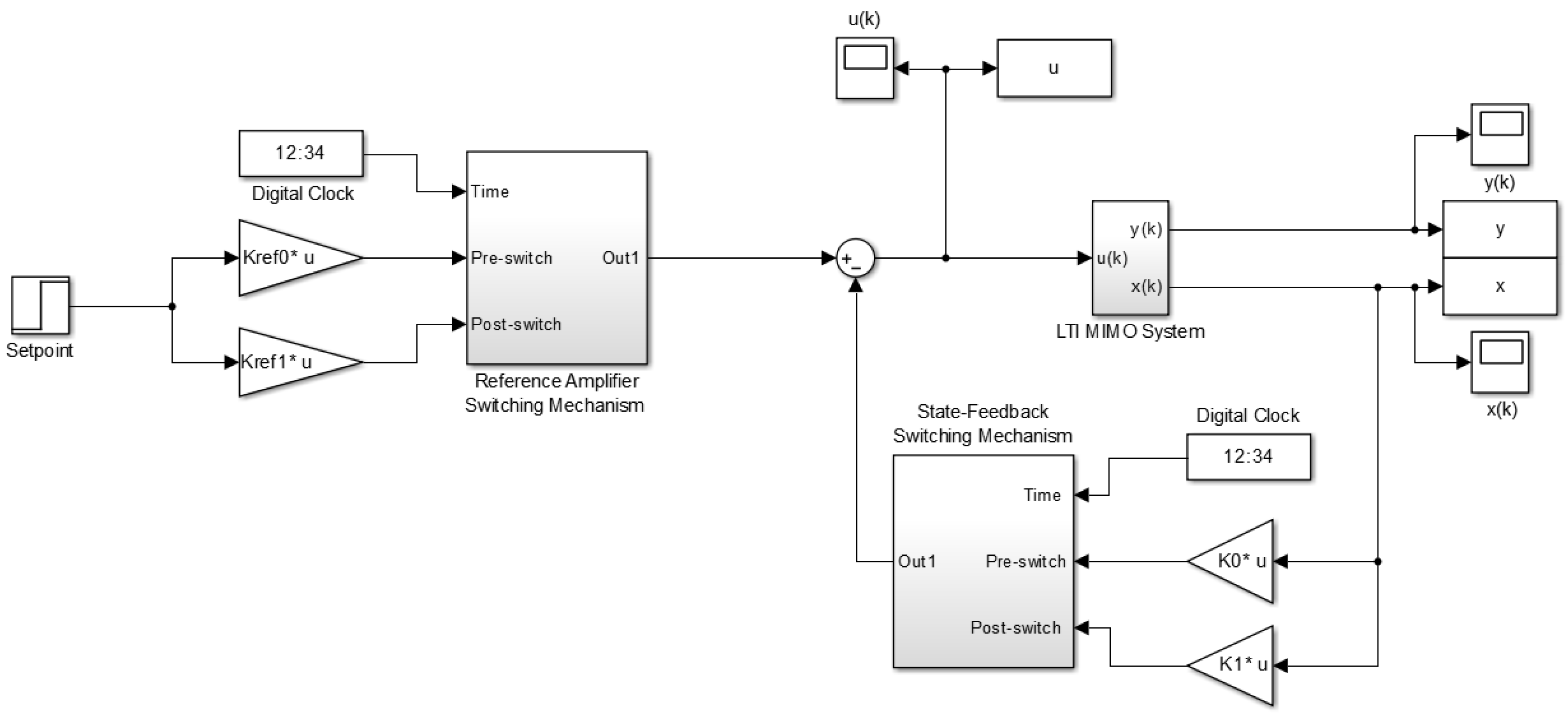
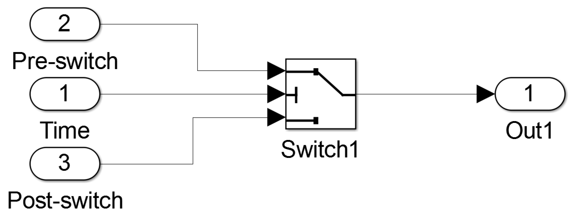
Having defined the basic properties of the switching perfect control system, let us continue with the application of the whole mentioned machinery into some particular MATLAB/Simulink simulation instances.

6. Simulation Examples

In this section, the simulation study concerning the switching perfect control is described. To cover the peculiarities coming from the considered control strategy fully, there is a need to acknowledge some certain factors. Of course, the main subject is the application of different inverses to steady and transient states. Later, the time of switching between starting and ending feedback gains will be arbitrarily changed in order to obtain different energy- and speed-based performance indices. Some energy characteristics can also be presented based on the dependencies of switching parameters. Additionally, the possible minimization of control amplitudes is also expected here. Of course, for every given system, the benchmark constituted by the minimum-norm instance will be given. Let us now continue with two numerical instances covering previously described procedures in the aspect of perfect control design.

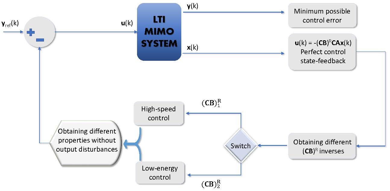
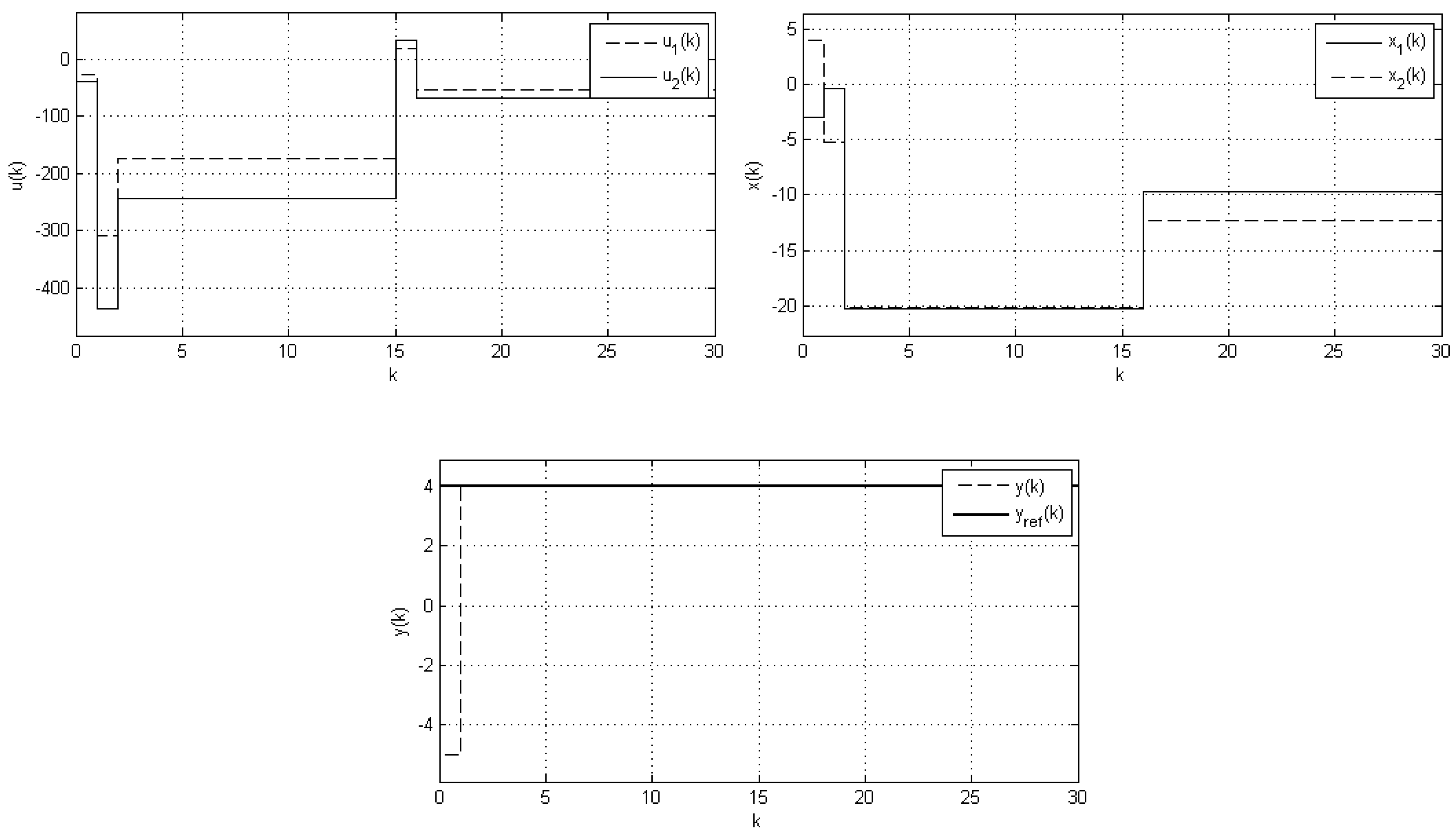
Example 1.

In the first simulation example, we are considering the LTI MIMO discrete-time system described with the following matrices$\mathbf{A}=\left[\begin{array}{cc}0.10& -0.40\\ 0.70& 1.20\end{array}\right]$, B = $\left[\begin{array}{cc}1.00& 0.50\\ -0.30& 0.80\end{array}\right]$, C = $\left[\begin{array}{cc}0.60& -0.90\end{array}\right]$$,and{\mathbf{x}}_0^T=\left[\begin{array}{cc}1& 2\end{array}\right].$ 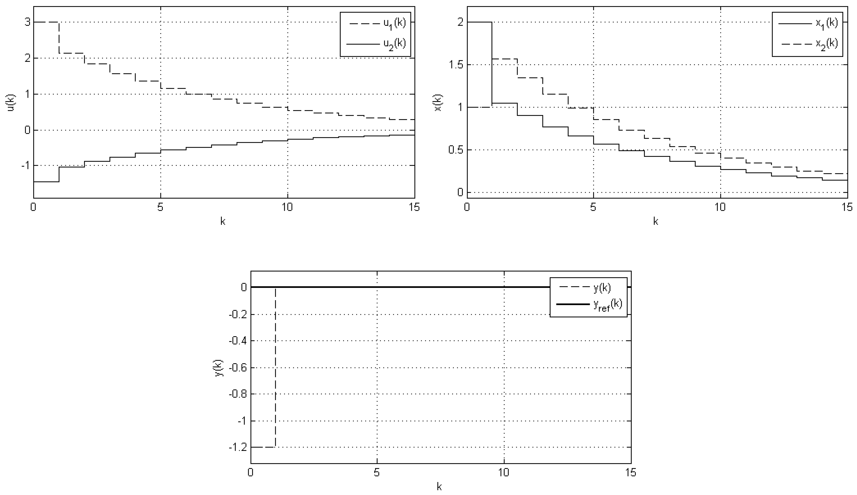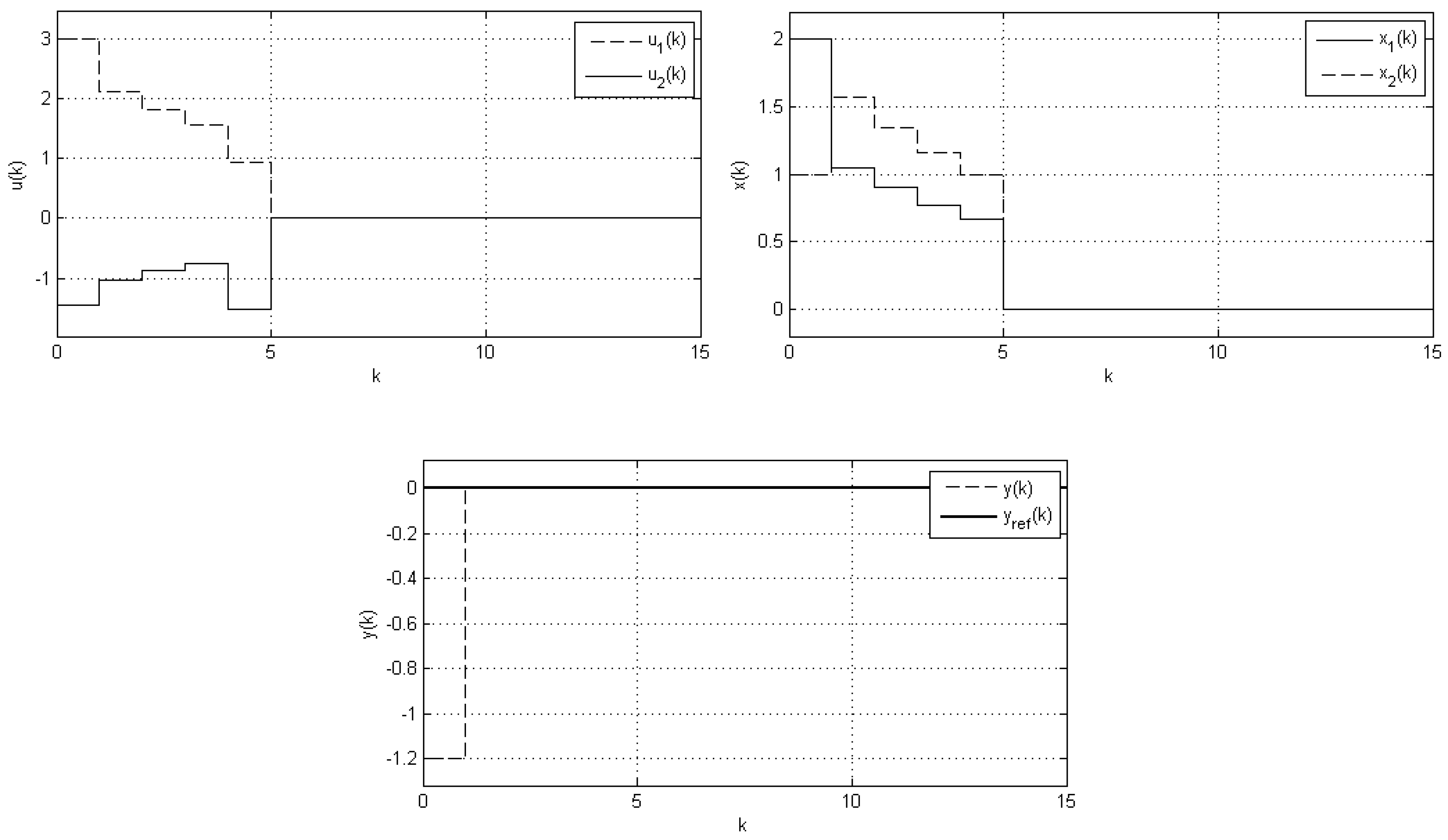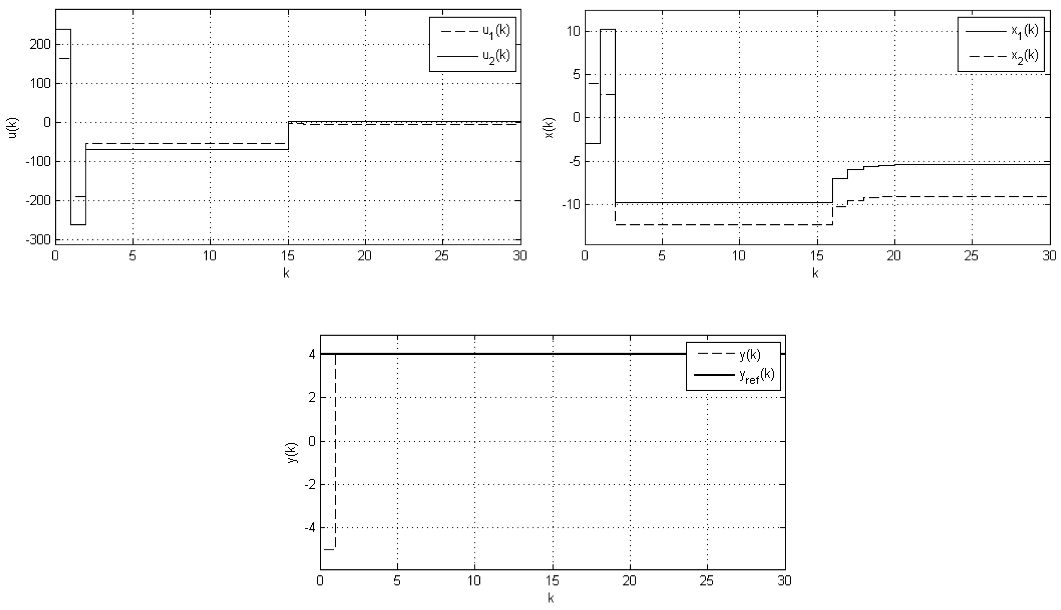With the application of the unique right T-inverse, we immediately obtain the state-feedback matrix equal to:

$$\mathbf{K}=\left[\begin{array}{cc}-0.5313& -1.2305\\ 0.2565& 0.5940\end{array}\right].$$

Now, according to the closed-loop formula of Equation (7), we arrive at the matrix describing the zero-reference perfect control plant as follows:

$${\mathbf{A}}^{\ast }=\left[\begin{array}{cc}0.5031& 0.5335\\ 0.3354& 0.3556\end{array}\right],$$

with eigenvalues equal to $z_1=0$ and $z_2=0.8587$. The corresponding control signals with the final energy $E_u=31.9681$ (in the squared ${\mathcal{L}}_2$-norm) and state variables are shown in Figure 1.

On the other hand, after application of the mentioned switching state-feedback methodology, under arbitrary selected degrees of freedom:

$${\beta }_1=\left[\begin{array}{c}0.8700-0.4200\end{array}\right],$$

$${\beta }_2=\left[\begin{array}{c}-0.76631.2579\end{array}\right],$$

applied to the state-feedback part of the IMC scheme, we arrive at the switching perfect control procedure. In such a case, the closed-loop system matrices are equal to:

$${\mathbf{A}}_1^{\ast }=\left[\begin{array}{cc}0.5031& 0.5335\\ 0.3354& 0.3556\end{array}\right],{\mathbf{A}}_2^{\ast }=\left[\begin{array}{cc}0.1655& -0.2483\\ 0.1103& -0.1655\end{array}\right].$$

Additionally, there is a need to define the last control parameter, namely the switching time $k_s$. Control and state signals obtained for $k_s=4$ under switching from ${\mathbf{A}}_1^{\ast }$ to ${\mathbf{A}}_2^{\ast }$ are presented in Figure 2.

In this scenario, the energy of the control signal is equal to $E_u=26.8649$. Indeed, with various degrees of freedom and switching times, different scenarios can be obtained. During the switching perfect control design, the proper selection of the transition time between two control gains can be crucial. Summing up, this simulation example clearly shows that the application of switching perfect feedback can result in measurable merits in terms of control speed and/or energy. Moreover, it is worth emphasizing that despite the change in state feedback, the output is preserved at its reference. These intriguing properties will be investigated in detail in the next perfect control instance. Of course, all results can be reproduced using the exemplary MATLAB/Simulink implementation given in Figure A1 and Figure A2, to be found in Appendix A.

Example 2.

In the second example, we take into account the nonzero reference/setpoint value applied to the perfect control algorithm dedicated to the state-space system with corresponding matrices

$$\mathbf{A}=\left[\begin{array}{cc}-0.30& 0.70\\ 0.40& 0.10\end{array}\right],\mathbf{B}=\left[\begin{array}{cc}1.20& -0.80\\ 0.20& -0.10\end{array}\right],\mathbf{C}=\left[\begin{array}{cc}-0.80& 0.60\end{array}\right],and{\mathbf{x}}_0^T=\left[\begin{array}{cc}4& -3\end{array}\right].$$

With the minimum-norm T-inverse-based perfect control design, we obtain the state-feedback matrix:

$${\mathbf{K}}_0=\left[\begin{array}{cc}0.8047& -0.2537\\ 1.0059& -0.3171\end{array}\right].$$

With such state feedback, the closed-loop perfect control system matrix is equal to:

$${\mathbf{A}}^{\ast }=\left[\begin{array}{cc}0.3781& -0.0063\\ 0.5041& -0.0084\end{array}\right].$$

Interestingly, the application of the already mentioned right T-inverse to the IMC-oriented plant with a nonzero reference value entails the setpoint pre-amplifier described by the following matrix:

$$\mathbf{B}{\left(\mathbf{CB}\right)}_0^{\mathrm{R}}=\left[\begin{array}{c}-3.3929\\ -2.8571\end{array}\right].$$

The corresponding state and control signals obtained for nonzero setpoint ${\mathbf{y}}_{\mathrm{ref}}\left(k\right)=4$ are presented in Figure 3.

Moreover, the switching procedure is applied here to the pre-amplifier. Thus, the setpoint gain is changed after switching time $k_s=15$ to the following value:

$$\mathbf{B}{\left(\mathbf{CB}\right)}_1^{\mathrm{R}}=\left[\begin{array}{c}-1.4127\\ -0.2169\end{array}\right].$$

In this scenario, the control energy is equal to $E_u=170.31e02$. However, the amplitudes of control signals seem to be more interesting, which are crucial for long-term control consumption. As we can observe, the switching gain parameter can influence the input behavior without any disturbances of the output variables.

Let us now consider the same setpoint amplifiers for the same LTI plant, but governed with different state feedback, i.e., for the state gain equal to:

$${\mathbf{K}}_1=\left[\begin{array}{cc}-0.4645& 0.4839\\ 0.1548& -0.1613\end{array}\right].$$

In such a scenario, the closed-loop perfect control system obtains properties that are different than in the T-inverse consideration. The only nonzero closed-loop pole is here equal to $z_1=0.3684$; hence, the system is stable. Naturally, the closed-loop poles are calculated as the eigenvalues of the closed-loop system matrix, which in this scenario is equal to:

$${\mathbf{A}}^{\ast }=\left[\begin{array}{cc}0.3813& -0.0097\\ 0.5084& -0.0129\end{array}\right].$$

For such a system, the switching control with $k_s=15$ resulted in the input and state variables presented in Figure 4.

Interestingly, in this scenario, the control energy associated with the nonzero reference value is equal to $E_u=1.5738e06$. Again, the control amplitudes can be decreased during the perfect control action without losing the proper output behavior.

The last considered simulation test covers the case where the state feedback is switched under nonzero reference. The key point of this study is to show that the linear gain matrix $\mathbf{K}$ affects the steady-states of control signals. Here, we are touching the same control system as before, but instead of setpoint gain, the state feedback is switched. With switching time, as before, equal to $k_s=15$, we adjust the state feedback from ${\mathbf{K}}_1$ to ${\mathbf{K}}_0$. The signals obtained under constant ${\left(\mathbf{C}\mathbf{B}\right)}^{\mathrm{R}}{\mathbf{y}}_{\mathrm{ref}}\left(k\right)$ are presented in Figure 5.

Again, the obtained results clearly show that the steady control amplitudes can be reduced with proper application of nonunique inverses. In this particular case, the energy of single steady control signal is decreased from $E_{15}=7675.2$ to $E_{30}=30.6090$ at every simulation step.

7. Summary and Future Work

The perfect control algorithm is a very interesting research area with plenty of possible developments. The classical inverse-based approach has already exhibited numerous advantages in terms of control speed, energy, or in general, robustness. In this paper, the perfect control design process was enhanced even more with the application of switching parameters.

The novelty of this manuscript mainly touched the nonzero referenced perfect control systems, which has never been attempted before. A number of simulation cases showed that the energy of control signals could be significantly limited, which is a key property in the perfect control design, since this control strategy was originally very energy-demanding.

Moreover, it is clear now that during the minimum-energy perfect control pursuit, it is necessary to find compromise between the energy of transient and steady-states. This compromise is usually given by some numerical solutions posed during the control design process. Amazingly, the merging of perfect and sliding mode control can stretch the boundaries usually applied to the mentioned energy-based consideration.

It was shown that the proper degrees of freedom, including the switching time, provided the perfect control scheme to be almost arbitrarily influenced aiming at different properties. Simultaneously, it is expected that some clear frameworks will be developed allowing obtaining the desired properties with the lowest possible computational effort.

Summing up, a new approach covering the switching perfect control was given in this paper. The new framework supported by a number of simulation examples clearly showed that the nonunique matrix inverses could have even a greater influence than in the classical method; thus, more studies employing this approach are expected in the near future.

The symmetric extension of the new solutions presented throughout the manuscript to the set of nonlinear plants also constitutes a solid research challenge. The second most import problem seems to be transferring the new issues to the case of the stochastic scenario involving the additive disturbance in the form of the uncorrelated zero-mean Gaussian-related white noise sequence, as many actual processes employ such a modeling paradigm. Last, but not least, the analytical objective function of the switching state-feedback control seems to be a real research challenge in the near future. Finally, in order to obtain the useful benefits of the new approach, the comparison with other control techniques in the form of classical perfect control or even classical sliding mode control is also required.