1. Introduction
The possibilities of unification of the early time inflationary era with late time accelerated expansion of the universe is one of the attractive facts of modified gravity theories; this captured the attention of the researchers in this field. This approach, based on geometrical grounds, avoids the introduction of additional degrees of freedom for the inflation or dark energy.
The modified gravity models represent an appealing alternative to a dynamical explanation of dark energy (for review see [
1,
2,
3,
4]), despite the success of the cosmological constant as the source of dark energy, but which is clouded by the known fine tuning problem. These theories introduce additional non-linear corrections to the Einstein model, which are subject to local systems tests and cosmological observational constraints that determine the viability of the model (see [
5,
6,
7,
8,
9,
10,
11] for reviews). A variety of models for modified gravity were proposed and some of them are [
6,
12,
13,
14,
15,
16,
17,
18,
19,
20,
21,
22,
23,
24,
25,
26,
27,
28,
29,
30,
31,
32]. Models that can satisfy both cosmological and local gravity constraints were proposed in [
31,
33,
34,
35,
36,
37], and exact cosmological solutions were studied in [
38,
39,
40,
41,
42,
43,
44]. Modified gravity with arbitrary function of the 4-dimensional Gauss-Bonnet invariant was introduced in [
45,
46,
47]. There are also models that attempt to unify early time inflation with late time acceleration, among which we can highlight: [
15] in which negative and positive powers of curvature were introduced in order to unify inflation and cosmic acceleration, in [
48] an extension of the Hu-Sawyki model [
31] was proposed that includes inflation and late-time accelerated expansion, in [
49] a modified gravity that unifies power-law curvature inflation with late-time
CDM epoch was considered, in [
36] a class of exponential modified gravity models was introduced, in which the inflation and accelerated expansion are present, a simple modified model with exponential gravity was considered in [
37,
50], a model with exponential and logarithmic corrections was considered in [
51] and constant roll inflation with exponential modified gravity was studied in [
52]. Unified models of inflation and dark energy with modified Gauss-Bonnet contribution were studied in [
45,
46,
47,
53,
54]. In [
55] a comprehensive study of the cosmological constraints for general
theory was performed, where a classification of
models was proposed, depending on the existence of the standard matter era and on the final accelerated state. The viability of several models was also analyzed by using the autonomous system approach. In [
56], local and cosmological constraints are discussed and the evolution of matter density perturbations was studied. A dynamical analysis and study of critical points for locally anisotropic cosmological models of modified gravity were carried out in [
57,
58].
The aim of this paper is to propose a simple viable model of
gravity that consistently describes both the inflationary epoch and the late time accelerated expansion of the universe, while satisfies the stringent local gravity constraints. This model contains a new exponential gravity correction that gives compatible with observations description of the cosmic evolution, mimicking the
CDM model, and
term [
32] that becomes relevant at high curvature and gives successful explanation of the early-time inflation. The viability of the model is shown in the (
) diagram which describes trajectories connecting the matter dominated saddle point at
,
with late-time de Sitter attractor at
and
. The model also satisfies the more stringent local gravity constraints.
This paper is organized as follows. In
Section 2 we present the general features of the
models, including the autonomous system and the relevant critical points for our study in terms of the
parameters. In
Section 3 we present the model, showing the conditions for viability and its trajectories in the (
)-plane, including some numerical cases of cosmic evolution. In
Section 4 we present some discussion.
2. Field Equations
The modified gravity can be the described by the following action
where
and
is the Lagrangian density for the matter component which satisfies the usual continuity equation. The equation of motion is given by
where
is the matter energy-momentum tensor assumed as
and
. The trace of Equation (
2) gives
Extracting the time and spatial components of Equation (
2) gives by the expressions
and
where dot represents derivative with respect to cosmic time. The effective equation of state (EoS) from these expressions is
where
and
p include both matter and radiation components, i.e.,
and
. The viability conditions begin with the stability which demands that
where the first condition is necessary to avoid change of sign in the effective Newtonian coupling, and the second is necessary in order to avoid tachyonic behavior of the scalaron and is also a condition of stability under perturbations, especially at the matter dominated epoch. In fact, the scalar particle associated with
, dubbed scalaron with mass
which in matter epoch or in the regime
, when
and
can be reduced to
which requires
. Apart from that, the model must be compatible with the observational evidence at both local and cosmological scales. The mass
M plays an important role in local gravity constraints since it defines the range of the force mediated by the scalaron which determines the Compton wavelength
. If
ℓ is the typical size of a local gravitational system, then the local gravity constraints on
are satisfied whenever
or
[
55,
56]. On the other hand, to demonstrate the viability of modified gravity as cosmological model it is useful to consider the autonomous system with the following dimensionless variables that can be obtained from Equation (
4) [
55] (we will use indistinctly
or
)
which lead to the following dynamical system
where
,
is the density parameter of the radiation component, and
m is given by
Along with the parameter
m there is another useful parameter
r defined as
These parameters are useful to analyze the cosmological viability of
models and characterize the deviation of a given
model from the standard
CDM model, which corresponds to the line
. In terms of the dynamical variables the effective EoS (
6) is written as
while the dark energy equation of state from (
4) and (
5) can be written as [
55,
56]
where
is the current value of
.
The critical points of the dynamical system (
11)–(
15), that are the solutions of the equations ([
55,
56])
allow analyzing asymptotic cosmological solutions of the model (
1) and their stability properties. Among the solutions of the system (
20) there are three important critical points that we will consider to analyze the viability of our models (in this analysis we do not consider the contribution of radiation, which does not change the stability properties of the critical points).
The first critical point corresponds to scaling solutions which include the matter dominated era, has the following coordinates in terms of the parameter
m
with eigenvalues
where
m is given by (
16) and prime represents derivative with respect to
r. At this point the matter density parameter and the effective EoS take the form
The second point has the coordinates
with eigenvalues
and lead to the de Sitter solution with
The third critical point, that leads to accelerated expansion scenarios, has the coordinates
with the eigenvalues
The matter density parameter and effective EoS corresponding to this point are
From the coordinates
y and
z for the points
and
it can be seen that they are connected by the line
, where the relation
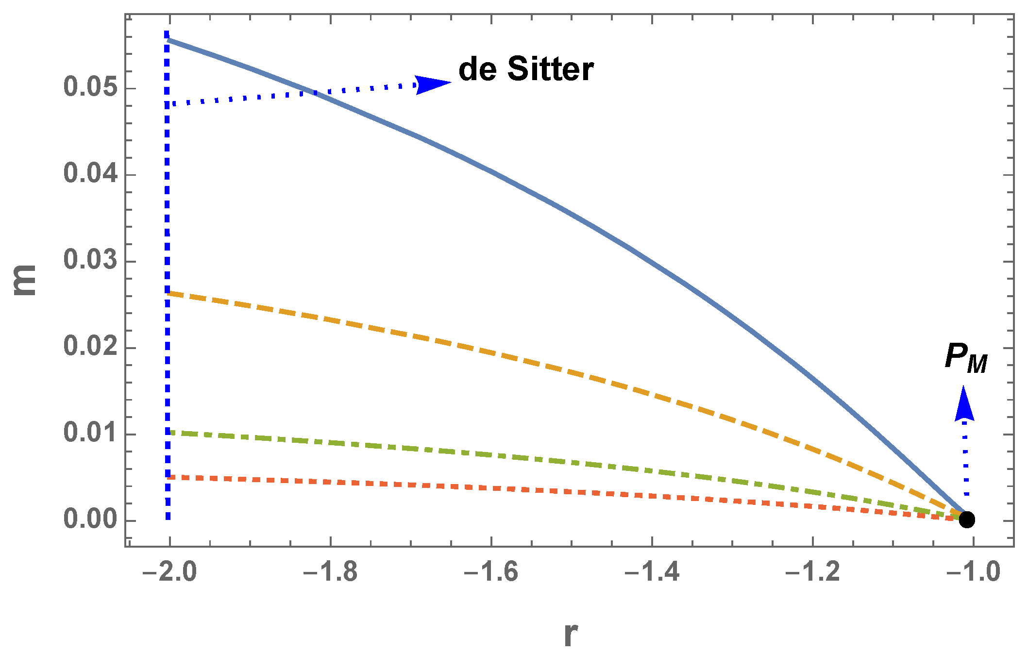
is used.
From (
21) follows that the matter dominated point corresponds to
=
. The existence of a viable saddle matter era requires
and
. This last condition implies that all the
trajectories must be between the lines
and
. In order to be viable, the trajectory of a given
model in the
plane should be such that it contains the matter dominated point
and starting from
intersects the line
in the region
[
55]. The
CDM model, for instance, connect the points
and
. There are also viable trajectories connecting the saddle matter point
with the curvature dominated point that leads to stable accelerated expansion
, whenever
.
3. The Models
The following model, as will be shown satisfies all above discussed conditions of stability and viability
where the dimensionless constants
,
and
are positive, and
. This function is well defined for any
R and describes the physical regimes related to the crucial cosmological epochs epochs of the universe: the inflationary regime where the relevant contribution comes from the
Starobinsky term and the small curvature regime covering from the matter era to the current stage of accelerated expansion, where gravity is described mainly by the first two terms in (
31). The Lagrangian composed of
which is the dominant sector of the model (
31) for large curvature, typical of the inflationary epoch, gives the well known and still consistent with observational data Starobinsky inflation. Hence, these two corrections are of different nature and are introduced for different purposes. Then to analyze the viability of the model to explain the late time accelerated expansion, the
term should be irrelevant, which imposes restrictions on the parameter
. In fact the scale
was introduced in the last term with the sole objective to make
dimensionless, since at the end
must satisfy the restrictions imposed by the curvature at the inflationary period. The properties of the model (
31) must be reflected in the behavior of the autonomous system, as we show below. First we note that the exponential function satisfies the limits
The first limit allows the existence of flat spacetime solutions and the second is necessary for consistency with high redshift CMB observations.
To check the stability conditions (
7) we analyze the corresponding expressions for
and
The condition
can be easily meet under the assumption
and taking into account that
. Since the last term in (
34) is positive and the
R-dependent terms are always less than 1, it can be satisfied under the following restriction on
From (
35) follows that
is always true for
and
. This is compatible with the criteria we will use below to redefine the stability conditions, by setting
such that the de Sitter critical point takes place at
.
The
r and
m parameters for the model (
31), that determine its cosmological viability, are obtained from (
17) and (
16) respectively and are given by
and
where the expressions for
and
from (
34) and (
35) were used.
To analyze the stability at the de Sitter point
, we fix
in such a way that the de Sitter point
takes place at
. From (
37) it is found
Please note that this value does not depend on
because de de Sitter solution is automatically satisfied by the
-model. The restriction
can be solved by imposing
And for the stability condition at the de sitter point
, using the above value for
, leads to
This inequality cannot be solved explicitly in terms of
, but it we choose the parametrization
which satisfies (
40), then the inequality (
41) becomes
that is satisfied by
In fact, given that
, this inequality is always satisfied by any
which is consistent with (
42).
Turning to the stability conditions and taking into account
from (
39) and
from (
42), we find after replacing in (
34)
as
, then a sufficient condition to satisfy the inequality
is
From the fact that
follows that
or
then the inequality (
46) also takes place if we assume the maximum value for
, which reduces to
which takes place if additionally to
, we impose the restriction
. For the second derivative
we obtain
And the stability condition
is automatically satisfied since
and
(we can also use the maximum value of
coming from the inequality
to find that
, which leads to
). Thus, we found the conditions for stability without compromising the constant
which will be useful in adjusting the Starobinsky
term with the scale of inflation. It is worth noticing that the stability condition
holds for any
, and there are not any instability problems related to the matter epoch and at local systems scales. Note also that the stability conditions derived after fixing
maintain the consistency with the general stability conditions derived for
and
given by the expressions (
34) and (
35) respectively. The restriction (
36) on
can be satisfied assuming, for instance,
(i.e.,
) one finds
To analyze the viability of the model in the
-plane we resort to the parametric plot of some trajectories, since
m cannot be expressed analytically in terms of
r. Using (
37) and (
38) and defining the variable
with de Sitter value
(see (
42)) we can write the corresponding expressions for
r and
m as follows
where we used the expression for
from (
39). It can be confirmed that at
,
r takes the value
. To simplify the numerical analysis, in what follows we assume the restriction
that satisfies all above restrictions and, according to (
42), gives
.
On the other hand, the value of
must be chosen in such a way that
where
, which is the typical value required for inflation. If
is the typical curvature during inflation, then the coefficient
should be of the order of
to ensure that in the small curvature regime, when
, it is verified that
necessary to avoid the effect of the
-term in the small curvature regime. Thus, for the model (
31) the physical criteria to establish the value of
involves the curvature (mass) scale
. At the same time, this scale is set so that local gravity constraints are satisfied. In any case since, after the restriction (
52), the de Sitter curvature satisfies
, then this scale should be smaller than the current curvature
, i.e.,
, which implies, according to (
53), that
In
Figure 1 we present some trajectories in the
-plane. The model contains the matter dominated point
and cosmologically viable trajectories that connect the matter era with the final de Sitter attractor at
. As can be seen from
Figure 1 the value of
is such that it avoids the effects of the
term during the matter era. Nevertheless numerical calculations show that the curves in
Figure 1 practically remain unchanged for any
, which reflects the fact that the scale
is not relevant for the cosmological trajectories in the
-plane. The real stringent restrictions on
, and therefore on
through (
53), come from the local gravity tests.
Local Gravity Constraints.
The effective mass corresponding to the modified gravity
model is given by
This mass characterizes the range of the force mediated by the scalaron and defines the Compton wavelength
. To avoid the propagation of this scalar degree of freedom and satisfy the local gravity constraints, this Compton length must be negligible small compared to the typical size of the system
ℓ,
. Thus, to satisfy the local gravity constraints it is necessary that
If we use the approximation for the local curvature
, then using this in (
56) we can write
then from (
57) it follows that
which gives from (
56)
This allows us to write the constraint (
57) as
Making use of the relationship
applied to the current universe (
) and to the local structure (
), we can write
and the above constraint becomes [
56]
For the solar system with gr/cm and cm one finds that , where we used cm.
Applied to the model (
31) the local gravity constraints can be addressed using the representation for
m given by (
51). For the solar system one has
, where
. For the parameters
and
p used in
Figure 1, we will set
, which gives
and
(assuming
in (
53)
Hence, the model (
31) can pass solar system tests, assuming
for the viable trajectories depicted in
Figure 1. If we consider larger values of
then the results for local systems improve as shown bellow.
It is worth noting that the above numerical values for local restrictions on
m can be obtained for
, even though
is subject to the restriction (
53) which results in much smaller values than this limit.
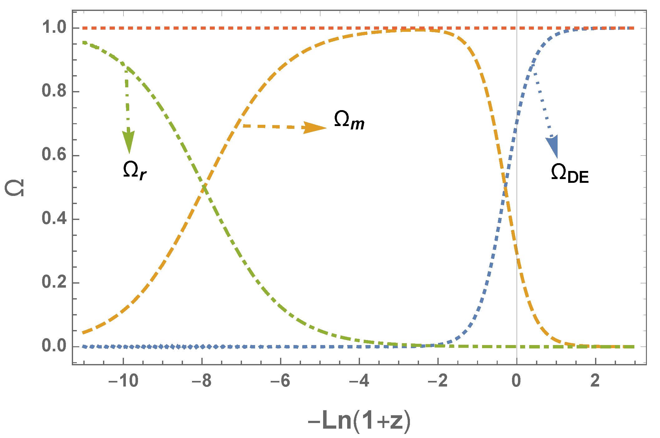
In
Figure 2 we present the evolution of the density parameters for the radiation
, matter
and the geometrical dark energy
, with parameters
and
p that satisfy cosmological constraints. Since there is no explicit expression for
, we used a polynomial fit to the paths depicted in
Figure 1. Taking, for instance, the cosmological scenario with
and
, the corresponding trajectory in
Figure 1 can be approximated by the following function of the dynamical variables
and
(
)
with
where (
) represents more digits taken into account for the numerical calculations.
Numerical calculations show that as in the case of the
-plane in
Figure 1, the evolution of the densities does not substantially change if we choose
(including
obtained after inflationary restrictions). This indicates that cosmological constraints on
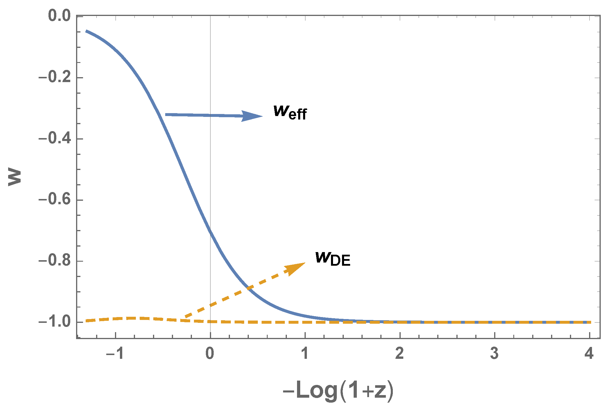
are not as stringent as local gravity constraints. In
Figure 3 we show the behavior of the effective and geometrical dark energy equations of state for this numerical sample.
Please note that these numerical results are consistent with those obtained in [
59], showing that the
corrections in the matter era are negligible. The
term is also consistent with local gravity tests according to the above numerical values of
m. It is worth noting that if we continue lowering the values of
, the model becomes practically undistinguishable from
CDM, but the local gravity constraints become more relaxed in the sense that the scale
does not have to be so small compared to
. Thus, we find the following behavior
In this case, the local restrictions on m can be obtained for .
Model 2.
A viable model with characteristics similar to those of the model (
31) has the following form
where as in the case of the model (
31),
and
. This model satisfies the limits
showing closeness to
CDM model with the cosmological constant vanishing in the flat spacetime. Let us first look at the model’s ability to produce inflation. To this end we consider the model
where the second term in (
66) was neglected. The corresponding scalar field in the Einstein frame has the form
The scalar potential in the Einstein frame for
models
gives for the model (
68)
Using parametric method, in
Figure 4 we show the shape of the potential, which maintains similarity with the Starobinsky potential and is appropriate for slow-roll inflation. The slow-roll parameters defined for the potential
take the following form using the variable
These parameters are evaluated at the horizon crossing where the curvatures takes the value
, i.e.,
. The inflaton value at the end of inflation is found from the condition
, which leads to the approximate equation for
where we neglected the exponential for
. Additionally if we consider
, then
and we ca appreciate the magnitude of the curvature at the end of inflation from
In the slow-roll approximation the duration of inflation is measured by the
e-folding number
N
where
is the curvature at the horizon crossing. Numerical integration gives
for a given number of
e-foldings before the end of inflation, sufficient to prove the viability of the model to predict the values of inflationary observables. The spectral index of scalar perturbations and the tensor-to-scalar ratio are among the most important observables and for the potential driven inflation are given in therms of the slow-roll parameters by
To evaluate
and
r we will consider the case with numerical parameters that were used to obtain the evolution of density parameters in
Figure 2 (
) (dotted line in
Figure 1) and that satisfy local gravity constraints (
) and
from (
53). We can use these results from the model (
31) because the intermediate matter era and the late time behavior is the same for both models, including the local gravity restrictions. After numerical calculations, taking
(suggested by (
76)) and
we find that
which gives, after replacing in (
73) and (
74),
which are in good agreement with the current Planck observations. From (
69) we find
and
. The corresponding Hubble parameter during inflation is
. Then the model is capable of describing inflation, matter era and late time accelerated expansion.
To analyze the stability conditions we first define the constant
in such a way that the de Sitter solution at
is reached at
. The
r and
m parameters take the form
where
. The equation
at
(
) gives
which lead to
for
Replacing
in
m (
81), the stability condition for de Sitter point,
leads to the inequality
To facilitate the numerical analysis, in what follows we will set
, equivalent to
. Setting
in (
84) we find
which given the fact that
, is satisfied by any
. The first derivative of
, after replacing
and setting
becomes
Since all the terms, except the last one, are positive then to satisfy the condition
it is enough that it is fulfilled
Since
, and
then the sufficient condition to satisfy
is
Repeating the same procedure with
we find
which automatically satisfies
since
,
and, according to (
83),
. Then the model (
66) satisfies all conditions of stability and cosmological viability.
Concerning the local gravity restrictions, for the solar system the model gives the same values for
m shown in (
63) and (
65). Likewise the density parameters and the equation of state, present the same behavior as shown in
Figure 2 and
Figure 3. As is the case for most of the realistic models, the stringent local gravity constraints forces the models (
31) and (
66) to be practically indistinguishable form
CDM. The possibility remains that further analysis of matter perturbations allows finding a departure from
CDM.
The exponential term in the models (
31) and (
66) is useful to avoid some type of singularities. Excluding the last term in (
31) and (
66) we can see that
as
,
tends to 1 and
at
. Then the r.h.s. of Equation (
4), excluding the matter density, for the models (
31) and (
66), which gives the corresponding
, tends to a constant value on singular solutions with
, avoiding in this way the appearance of type I and type III future singularities [
37]. From
Figure 1 and
Figure 2 it is clear also that the inflationary term in the models (
31) and (
66) does not have any influence on the stability of matter era.
4. Discussion
Two models of modified gravity that are able to explain early time inflation and late time accelerated expansion were studied. The models include an exponential function of de form and the term. The factor , which is present in both models, leads to the limit at implying the disappearance of the cosmological constant. i.e., the models contain the flat space-time solution. The stability, cosmological viability and local gravity restrictions were studied. The dynamical system was solved under appropriate initial conditions, and the cosmological evolution for the density parameters corresponding to radiation, matter and (geometrical) dark energy was obtained, which is closely adjusted to current observations. Consequently, the equation of state evolves according to observations with showing the transition to the accelerated phase at the currently observed , and .
The local gravity constraints, as expected, impose very stringent conditions for
m to achieve values of the order
, which demand very small values for the scale
(
), although this scale may increase as we take smaller values of
. However, at the same time, making
smaller brings the model closer to
CDM, making it practically indistinguishable from it. In any case the general result is that the stronger the local gravity restrictions are, the further in the future the final de Sitter attractor of the system is. It is also interesting to note that the numerical results for local restrictions on
m can be obtained for
, even though
is subject to the restriction (
53) which results in much smaller values than this limit. On the other hand, the cosmological constraints, which do not depend on the scale
, impose softer conditions on
, being sufficient to consider
.
The expressions for
m given by (
51) for the model (
31) and by (
81) for the model (
66) suggest a correlation between the curvature dependent parameter
m and
, which could be useful to fix
by local gravity constraints on
m. This is an interesting alternative mechanism to fix
, other than the condition (
53) where the mass
is determined from the amplitude of the scalar power spectrum. On the other hand, at high curvature typical of inflation, the model (
31) leads to the Starobinsky inflation while the model (
66) gives a new potential with the appropriate behavior to develop successful slow-roll inflation. A peculiarity of this potential is its dependence on
and
that is transferred to the slow-roll parameters, allowing exploring a wider region of possibilities for the inflationary observables, compared to the Starobinsky potential.
A more detailed analysis of local gravity restrictions is necessary, particularly to test whether local gravity constraints can independently and uniquely determine a value of that is consistent with inflation. Further study of cosmological effects that distinguish the models form CDM is needed, for instance, the evolution of the background and matter density perturbations which could give patterns in the growth of structures that mark the difference with CDM.


