Symmetric Free Form Building Structures Arranged Regularly on Smooth Surfaces with Polyhedral Nets

Abstract

The article is an original insight into interdisciplinary challenges of shaping innovative unconventional complex free form buildings roofed with multi-segment shell structures arranged with using novel parametric regular networks. The roof structures are made up of nominally plane thin-walled folded steel sheets transformed elastically and rationally into spatial shapes. A method is presented for creating such symmetric structures based on the regular spatial polyhedral networks created as a result of a composition of many complete reference tetrahedrons by their common flat sides and straight side edges arranged regularly and symmetrically in the three-dimensional Euclidean space. The use of the regularity and symmetry in the process of shaping different forms of (a) single tetrahedral meshes and whole consistent polyhedral structures, (b) individual plane walls and complex elevations, (c) single transformed folds, entire corrugated shell roofs, and their structures allow a creative search for attractive rational parametric solutions using a few author’s parametric algorithms and their implementation as built-in commands of the AutoCAD visual editor or applications of the Rhino/Grasshopper program.

1. Introduction

Thin-walled steel sheets are profiled in one direction to use them as members and coverings for roofing. The rationality of using such sheets results from the very favorable ratio of self-weight to load-bearing capacity or covering surface area, and from quick roof assembly [1]. Due to the orthotropic properties of the sheeting, including very different stiffness in two orthogonal directions, flat profiled sheets have been elastically deformed into two shell forms, i.e., rotational cylinder [2,3], Figure 1, and central sectors of right hyperbolic paraboloids [3,4], Figure 2.

Geometric and mechanical changes of the transformed sheets depend on the imposed boundary conditions including the type and degree of the shape transformations. The possibility of using elastically deformed folded sheets as roof coverings depends primarily on the amount of the initial stresses caused by the shape transformations. Therefore, shallow hyperbolic paraboloid sheeting shaped as a result of small twist transformations are most often used [2], Figure 2.

Thin-walled steel sheets having open profiles and folded in one direction can be joined with their longitudinal edges into nominally flat sheeting and transformed into ruled shell shapes as a result of spreading onto at least two skew roof directrices, Figure 3a. The shell shape of each transformed sheeting depends on a mutual position and curvature of two edge directrices. The sheeting can be modeled with a regular smooth ruled undevelopable surface called a warped surface [1], Figure 3b.

The analyses related to a static strength work of such deformed and loaded corrugated shells are based on analytical methods leading to calculations of critical forces [5] or FEM describing the entire behavior of these shells [6]. All spatial shape transformations investigated in the present article are effective because freedom of the transverse width increments of each shell fold diversified along its length is ensured [7]. The effective shape transformations are accomplished to obtain a rational static strength work of each shell fold and then very attractive visual building forms [8]. Each shell sheeting transformed effectively, Figure 4, is characterized by a line of contraction passing through the half-length of each shell fold and the smallest possible pre-stresses [9].

The specific feature of the investigated effective shape transformations is that they particularly provide an easy shaping of various symmetric unconventional and rational shell-free forms of roofs, entire buildings, and their structural systems [10], Figure 5a,b. In this way, very attractive free forms of buildings having oblique eaves, girders, and elevations can be shaped [11].

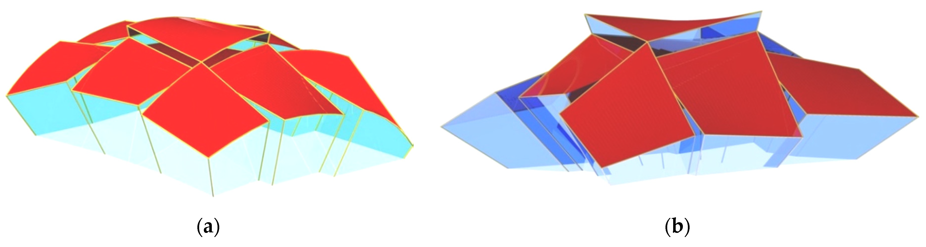
The aforementioned basic properties and restrictions of a rational shaping of single corrugated ruled shell-free forms transformed effectively, concerning the complexity of their shapes, including the contractions, results in the fact that two complete corrugated shell sheets cannot be joined with their crosswise ends, that is perpendicular to their fold’s direction, to obtain one resultant smooth shell [3]. Straight or curved edges must appear between two individual shell sheeting joined transversally towards their folds, Figure 6a. Thus, such shells must be modeled by means of complex multi-segment roof shell structures, Figure 6b.

2. State of the Art

Thin-walled folded steel sheets of open profiles allow easy deformations of their folds, including their flat rectangular walls and inclination angles between flanges and webs. Nilson studied the possibilities of the sheet’s deformations into hyperbolic paraboloid shells and published his research in 1962 [12]. He showed that double-layered fold sheeting transformed elastically into a central sector of a hyperbolic paraboloid or a symmetrical arrangement of four quarters of such a sector is more economical than a reinforced concrete hyperbolic paraboloid shell.

The research conducted under the guidance of Winter [13] confirmed the most important Nilson’s conclusions. It was associated with a greater variety of the sheet profiles and dimensions of two-layer hyperbolic paraboloid shells. Central sectors and compositions of quarters of the hyperbolic paraboloid shells were examined. Parker studied roof structures consisting of four folded quarters of a right hyperbolic paraboloid. The analyzed segments were made of two layers of sheets located orthogonally and stiffened with a circumference frame. He analyzed the behavior of the transformed sheeting, including the changes in stiffness and potential energy of these sheets [4]. The Muscat’s research [14] concerned primarily critical loads and stability of the sheeting of the type analogous with the one investigated by Parker and Nilsen. Banavalkar made a thorough analysis of the static strength work of these shells [15].

A comprehensive summary of the research performed at Cornwell University is the report made by Gergely et al., [16]. The authors carried out a complete detailed analysis of the static strength work of single and complex profiled hyperbolic paraboloid shells. These shells were made up of plane sheets profiles located in two mutually orthogonal layers, which enables these researches to analyze the shells as isotropic. They examined folded shells of different profiles.

Behavior of a central sector of a folded steel hyperbolic paraboloid stiffened with a circumferential frame was studied by McDermott [17]. Gioncu and Petcu [18] studied the work of the analogous hyperbolic paraboloid shells using traditional analytical analyses of strength and critical loads. They finally developed a novel HYPBUCK computer program for calculating critical loads. They also studied umbrella shell sheeting composed of four symmetrical right hyperbolic paraboloid quarters in various configurations, Figure 7a,b.

Parallel studies and analyzes related to the static strength work of single and complex hyperbolic paraboloid shells made up of flat folded sheets of different profiles were conducted by Egger et al. [19]. Their method is based on the performed tests, conventional analyses, and analytical calculations of strength and critical loads.

The shells investigated by the aforementioned researchers were undergone forced shape transformations causing relatively big pre-stresses due to the imposed boundary conditions, including the joints between two orthogonal layers arranged over the whole area of the transformed shells and the frames stiffen the quadrangular edges of the shells, so only shallow hyperbolic paraboloid shells called hypars could be created, Figure 8a,b. In addition, the adjustment of all longitudinal shell fold’s axes to the calculated rulings of the designed hyperbolic paraboloid quarters imposes a significant change in the width of the transverse fold’s ends passing along each shell directrix affecting important initial stresses. To limit the level of the pre-stresses, a maximum deformation degree has to be introduced. Initial forced deformations of the nominally plane folded sheets have been used by Dawydov in prefabrication of long-span roof panels [20].

Davis and Bryan [21] described the most important geometrical and mechanical characteristics of flat and thin-walled transformed shell folds. They presented a complete way of analyzing and designing shells and structures made up of two-layer corrugated sheets located orthogonally. Two most important general conclusions given by these authors and regarding the transformed roof shells are as follows. The researchers found that, theoretically, it is possible to shape many different types of the transformed folded shell sheeting. Practically, however, it is possible to build only cylindrical and hyperbolic paraboloid types of the transformed folded steel shells for roofing due to the available technology.

The use of the well-known conventional design methods [1,16,19,21], known from the traditional courses of theory of thin-walled shells, in shaping of such transformed shell roofs is ineffective because it usually results in high values of normal and shear stresses, local buckling and distortion of thin-walled walls: flanges and webs. The assembly of each designed shell sheeting into skewed roof directrices is often impossible because of the plasticity of the fold’s edges between flanges and webs. Reichhart developed a specific method for calculating the arrangement and the length of the supporting lines of all folds in transformed one-layer corrugated shell sheeting [10], Figure 5a and Figure 6a,b. The method is based on the orthotropic geometric and mechanic properties of the folded sheets and limits the value of the pre-stresses. His method enables one to shaped right hyperbolic paraboloids or other deep right ruled surfaces [22].

The Reichhart’s method is effective only for the cases where the fold’s longitudinal axes are perpendicular to roof directrices or very close to those [3]. The method leads to serious errors as it is demonstrated by Abramczyk [3]. These errors result from the lack of conditions providing similar values of stresses at both transverse ends of the same fold. Abramczyk significantly improved the Reichhart’s concept and has proposed an innovative method [3,8], so that the transformation would cause the smallest possible initial stresses on the shell folds resulting from this transformation. The visible result of different stress values at both transverse ends of the same shell fold is that the transverse contraction of the fold does not pass halfway along its length, on the contrary, it is shifted closer to one of these ends.

In order to create a method for shaping the considered type of the roof shells transformed rationally, Abramczyk [3] proposed a condition requiring the contraction of each entire shell to pass halfway along the length of each shell fold, Figure 3a,b. The condition has to be ensured to obtain a shell fold characterized by the effectiveness of the shape transformations [23]. The Abramczyk’s method employs some specific geometric properties of warped surfaces, primarily their lines of striction. The second condition utilized by Abramczyk relates to calculations of the respective surface areas modeling compressing and stretching zones on the transformed folds [24]. Both conditions are based on the results of his experimental tests and computer simulations [25], Figure 1 and Figure 2. They are implemented in the Abramczyk’s application [23] developed in the Rhino/Grasshopper program used for parametric modeling of engineering objects.

Simple shell structures composed of a few complete corrugated shells were used in different architectural configurations, most often as shells supported by stiff constructions based on very few columns [24,25]. Such shell structures are used for achieving (a) large spans; (b) greater architectural attractiveness; and (c) skylights letting sunlight into the building interior. Reichhart arranged the complete corrugated shells on horizontal or oblique planes [10] to achieve continuous ribbed structures, Figure 6 and Figure 9. He developed a simple method for geometrical and strength shaping of the transformed shell roofs. He designed a few corrugated shell sheeting supported by very stiff frameworks or planar girders with additional intermediate directrices, members, and roof bracings.

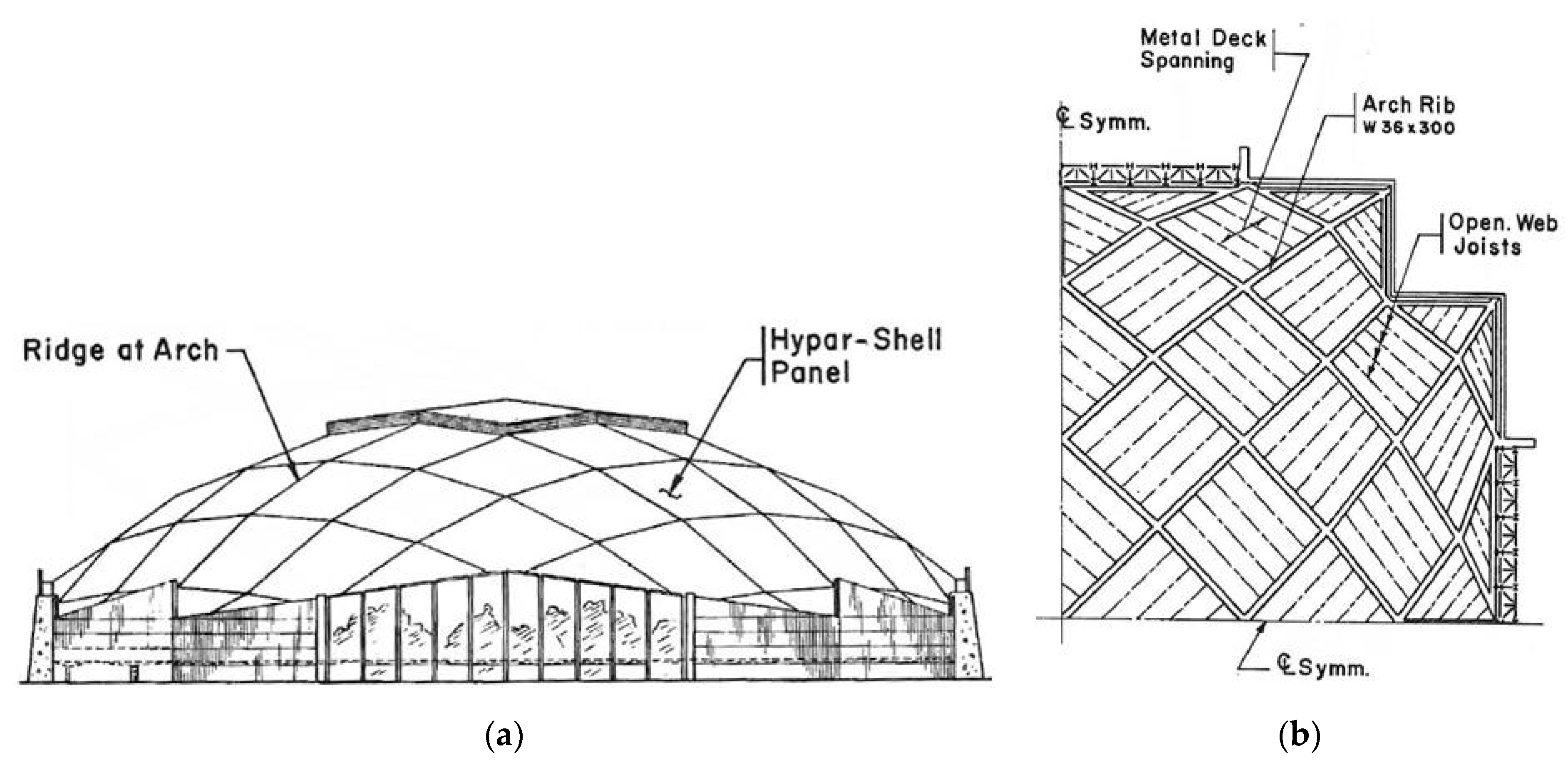
In the 70s, Biswas and Iffland [26] presented two concepts of two continuous regular roof structures composed of many identical hyperbolic paraboloid segments made up of transformed folded steel sheets arranged on two various spheres. In the first concept, Figure 10a,b, they proposed triangular shell segments having three-segment edge lines. Another important feature of this concept is that the proposed plane system, dividing the roof structure into tetrads of triangular shell segments, which is based on a sphere. This concept requires significant oblique cuts and big transformation degree of all rectangular folded sheets.

In the second concept, typical quadrilateral transformed hyperbolic paraboloid segments are used, Figure 11a,b. This concept is more realistic, but the degree of twisting and deflection of the complete hyperbolic paraboloid segments are small.

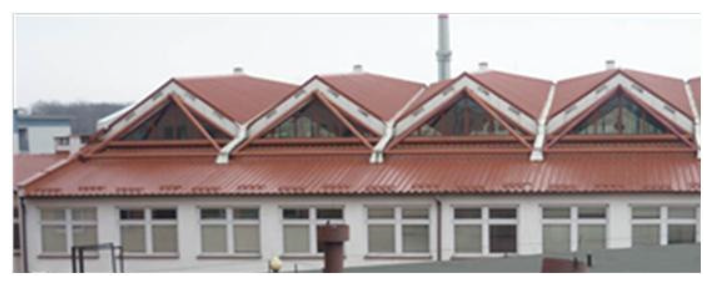
At present, shell structures consisting solely of steel decks are not visually appealing. In order to increase their attractiveness, it is possible to use: (1) areas of discontinuity between the metal steel segments, filled with, e.g., glass panels, (2) green plant gardens on the transformed segments, (3) coat the segments with different plastic membranes, (4) communication routes between the segments, (5) a coherent connection of glass facades and steel shell roof.

In order to create medium and long span free form building structures roofed with complex corrugated shells, Abramczyk [27,28] has proposed certain types of the so-called reference tetrahedrons to model complete free forms covered with folded glass elevations and roofed with complete transformed corrugated steel shell sectors. These tetrahedrons can be arranged regularly in the three-dimensional space to model complex building free forms, Figure 12a,b. Prokopska [29,30] has drawn drew attention to the architectural aspects of shaping such forms.

One of the Abramczyk’s methods [31] relates to positioning of many aforementioned reference tetrahedrons along ellipses t₀ and w₀ contained in two orthogonal principal planes (x,z) and (y,z) of symmetry of a reference ellipsoid ω_r, Figure 13a. The method allows the investigated form of a polyhedral structure to be a regular network and precisely take into account by the designer the variable curvature of ω_r. The method replaces a finite number of the selected straight lines t_i,j normal to ω_r with side edges k_i,j of the sought-after reference tetrahedrons. A specific feature of the reference tetrahedrons is that two their subsequent straight side edges k_i,j and k_i+1,j belonging to the same side must intersect, while two corresponding straight lines t_i,j and t_i+1,j normal to ω_r do not intersect to each other, Figure 13b. The positions of t_i,j and t_i+1,j have to be replaced by k_i,j and k_i+1,j, so that the positions of k_i,j and k_i+1,j have to be defined based on the geometric properties of ω_r. An architectural study of a free form created with the help of the method is presented in Figure 14.

Parameterization of the reference tetrahedrons enables to computationally search for attractive unconventional building free forms [23,27] and innovative structural systems intended for the investigated complex building free forms. In the analyses of these systems, the supported himself with the following works Obrębski [32] developed a few methods for shaping very diversified shell rod structures. Rebielak [33] developed steel rod structural systems supporting flat roof covers composed of corrugated sheets. A team of researchers led by Abel and Mungan [34] published comprehensively many examples of the construction systems associated with shaping very diversified roof shells and building free forms. A parametric method for shaping rod shells in the form of Catalan surfaces using the Rhino/Grasshopper program is presented by Dźwierzyńska and Prokopska [35]. The exact geometrical characteristics and methods for determining regular curves and surfaces have been presented by Carmo [36] and Gray [37].

Transformed folded steel sheets are also used as curved supports for shell panels of individual roof covers [38], Figure 15. Convex roof shells characterized by the positive Gaussian curvature can be created in this way.

3. Aim

The aim is to present a novel method for parametric shaping of building complex free forms based on the innovative spatial polyhedral networks. The presentation is focused on using symmetry for (1) obtaining attractive complex shapes of shell roof structures, folded multi-plane elevations and entire free form buildings, (2) reducing the number of the variables required to define the geometric objects employed, (3) making the proposed algorithm very intuitive, (4) getting rationality of the transformed shell roof forms and their structural systems. The shell roof structures designed with the help of the method are composed of many complete shell sectors arranged in conformity with shapes of various regular reference surfaces. In addition, each elevation should be composed of many planar and oblique walls coherent with the designed shell roof structure.

4. Concept of the Method

The algorithm of the investigated method allows a rational use of the shape transformations of nominally flat thin-walled open folded steel sheets to achieve visually attractive shell roofs whose shapes determine unconventional building free forms as well as their innovative structural systems. Since any two roof directrices are mutually skew straight or curved lines, it is convenient to contain these directrices in the planes of façade walls or in the planes of roof girders. The directrices should be assumed as segments of the roof shell eaves. In addition, a controlled inclination of all elevations to the vertical makes it possible to increase the attractiveness of the created free form buildings.

A smooth resultant shell cannot be the result of a composition of two transformed individual shells with their transverse edges due to the location of the fold’s contraction of each effectively transformed roof shell with respect to the roof directrices. Thus, both smooth shells must be separated by a common rib disturbing the smoothness of the resultant complex structure. The ribs- between many complete transformed shells can be taken for common directrices of many pairs of the adjacent shells in the complex roof shell structure.

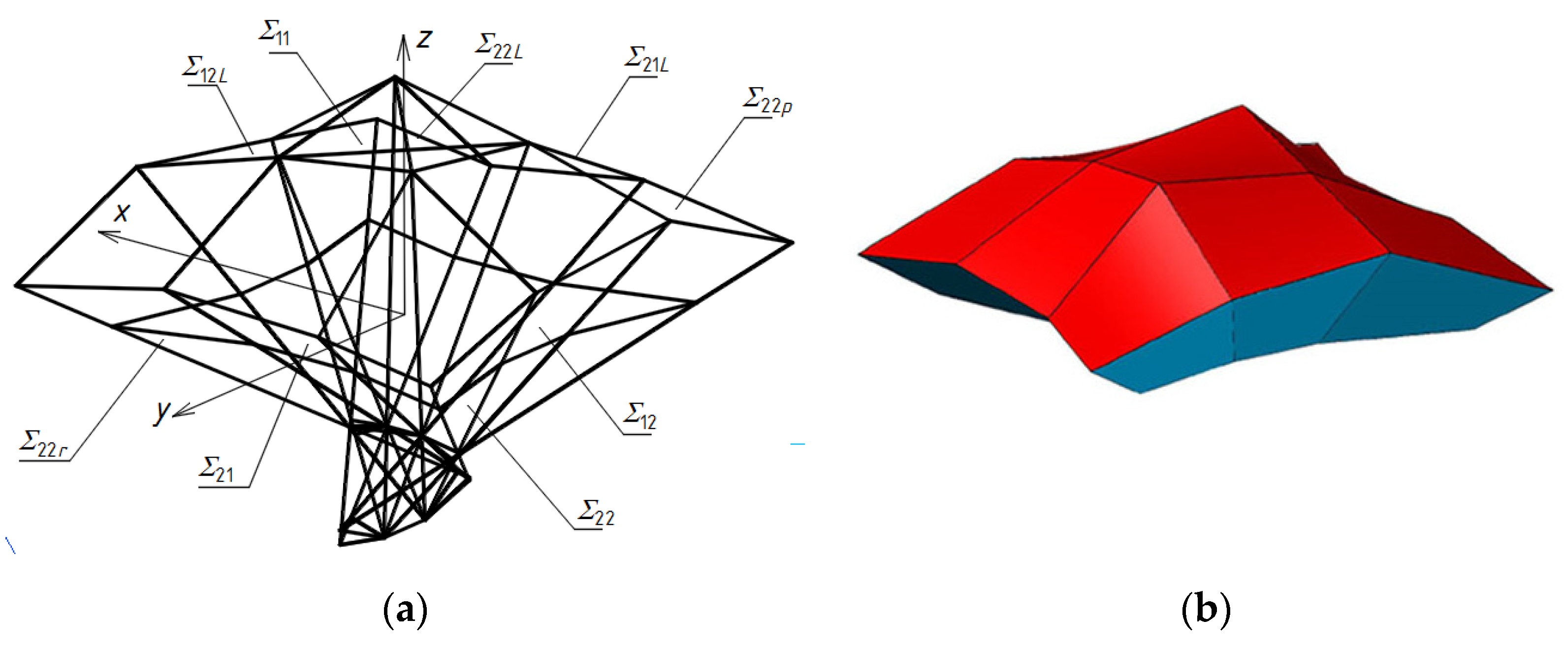
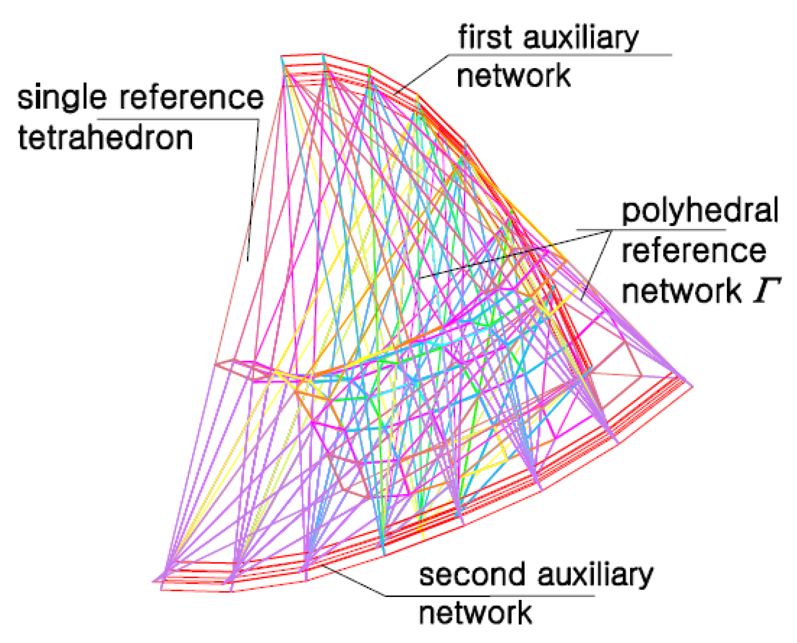
Following the method’s algorithm, a system of the planes separating all roof shell segments and containing the aforementioned edges, including directrices, has to be adopted. Such a spatial system is called a polyhedral reference network Γ. Each reference network Γ is characterized by the following geometrical properties. Each complete mesh Γ_ij of Γ is limited by four adjacent planes of the system defined by means of four vertices W_ABij, W_CDij, W_ADij, and W_BCij, Figure 16. Each single shell segment Ω_ij and each complete free form Σ_ij are located in one mesh Γ_ij, so that façade walls, roof directrices and eaves segments are included in the aforementioned quadruple of planes of Γ_ij.

Every two adjacent planes of each single mesh Γ_ij intersect in the side edges: a_ij, b_ij, c_ij, d_ij, and, every two opposite planes intersect in the axes u_ij or v_ij of Γ_ij. The side edges and axes of Γ_ij are defined by means of four vertices W_ABij, W_CDij, W_ADij, W_BCij, Figure 16a. Thus, each possible triple of these vertices determines one plane of Γ_ij. On the basis of these vertices, four points S_Aij, S_Bij, S_Cij and S_Dij are constructed on four side edges a_ij, b_ij, c_ij, d_ij. These points are vertices of a spatial quadrangle S_AijS_BijS_CijS_Dij determining a certain piece of a reference surface ω_r, Figure 16b. In relation to ω_r, four vertices A_ij, B_ij, C_ij, D_ij of single eaves B_vij are determined to obtain mutually skew roof directrices. Vertices P_Aij, P_Bij, P_Cij, P_Dij, Figure 16a, belonging to a flat horizontal base of the sought-after free form Σ are constructed in relation to the aforementioned four vertices W_ABij, W_CDij, W_ADij, W_BCij. The complex free form Σ created on the basis of such a reference network Γ is a sum of all individual free forms Σ_ij. Finally, a resultant z-axis symmetric free form structure can be achieved, Figure 17a,b.

Parameterization realized in the process of the geometric shaping of such free forms Σ is based on a definition of a finite set of variables entering into computer application in the form of either the measures of stiff motions, like rotations and translations, or division coefficients of all pairs of the adopted vertices of Γ. An algorithm of the stiff motions leading to the creation of Σ is presented in Section 5. An example of using the division coefficients in creating a spatial reference network is presented in Section 6.

5. Method’s Algorithm

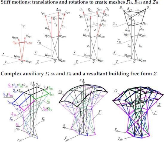
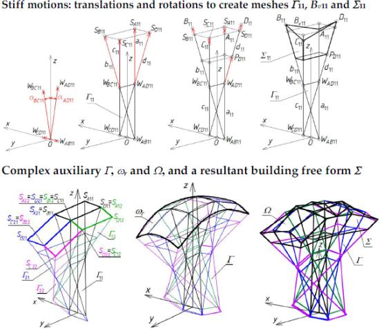
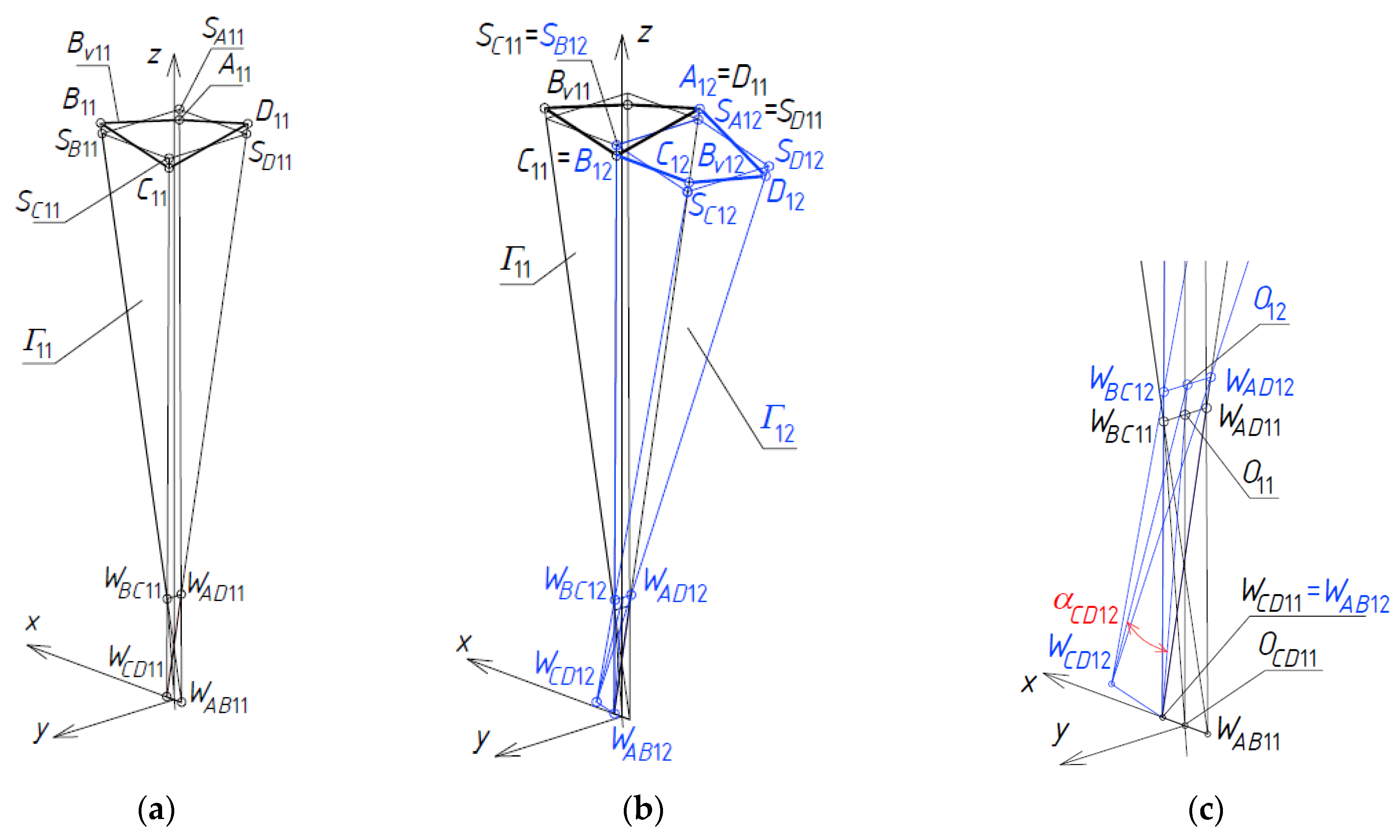
In the first step of the method’s algorithm, the first mesh Γ₁₁ of a reference network Γ is created so that the positions of its four vertices W_AB11, W_CD11, W_AD11, and W_BC11 are defined in the three-dimensional space. For this purpose, a global coordinate system [x,y,z] must be taken, Figure 18a, where a point O is the origin of [x,y,z]. These vertices are arranged symmetrically in relation to the principal planes of [x,y,z], so the sought-after mesh must be symmetric. The first set of initial data is formed from the measures of the vectors and angles employed to determine all characteristic points of Γ₁₁.

On the basis of the aforementioned set of initial data, four vertices of Γ₁₁ are determined as follows. The position of vertex W_CD11 is the result of the translation T_OCD11 of the point O by the vector OW_CD11 whose measure is defined by means of one element of the first initial set. In an analogous way, the position of vertex W_AB11 is defined by means of the translation T_OAB11 of the point O by the vector OW_AB11 so that its location is on opposite side of O on the x-axis.

The position of vertex W_AD11 is the result of a composition of the rotation O_{CD11_ AB11} of the z-axis about the x-axis by the angle α_AD11 and the translation T_OAD11 of O by the vector OW_AD11, where the measures of α_AD11 and OW_AD11 are two elements of the first set of initial data. The position of vertex W_BC11 can be obtained in an analogous way, that is, by means of the rotation O_{AB11_CD11} of the z-axis about the x-axis by the angle α_BC11 opposite to α_AD11 and the translation T_OBC11 of O. If we want to achieve a z-axis-symmetric reference tetrahedron, the absolute values of the above vectors and angles must be equal to each other, respectively.

The obtained vertices W_AB11, W_CD11, W_AD11 and W_BC11 determine four straight side edges: a₁₁, b₁₁, c₁₁ and d₁₁ of Γ₁₁. In order to obtain four points S_A11, S_B11, S_C11 and S_D11 of a reference surface and four vertices A₁₁, B₁₁, C₁₁ and D₁₁ of eaves B_v11 of a shell roof structure, four vectors have to be measured along the side edges a₁₁, b₁₁, c₁₁ and d₁₁, Figure 19a,b, so that S_A11= T_SA11(W_AD11), S_B11 = T_SB11(W_BC11), S_C11 = T_SC11(W_BC11), and = T_SD11(W_AD11), and A₁₁ = T_A11(S_A11), B₁₁ = T_B11(S_B11), C₁₁ = T_C11(S_C11), and D₁₁ = T_D11(S_D11). The measures of these vectors belong to the set of initial data.

In order to determine a horizontal plane base of the complete free form Γ₁₁, a point P_D11 = T_PD11(W_CD11) has to be defined on d₁₁. The measure of the vector W_CD11P_D11 must be one of the elements of the first set of initial data. Other points of this base can be calculated as the intersection of the horizontal base plane passing through the point P_D11 and the four side edges of Γ₁₁.

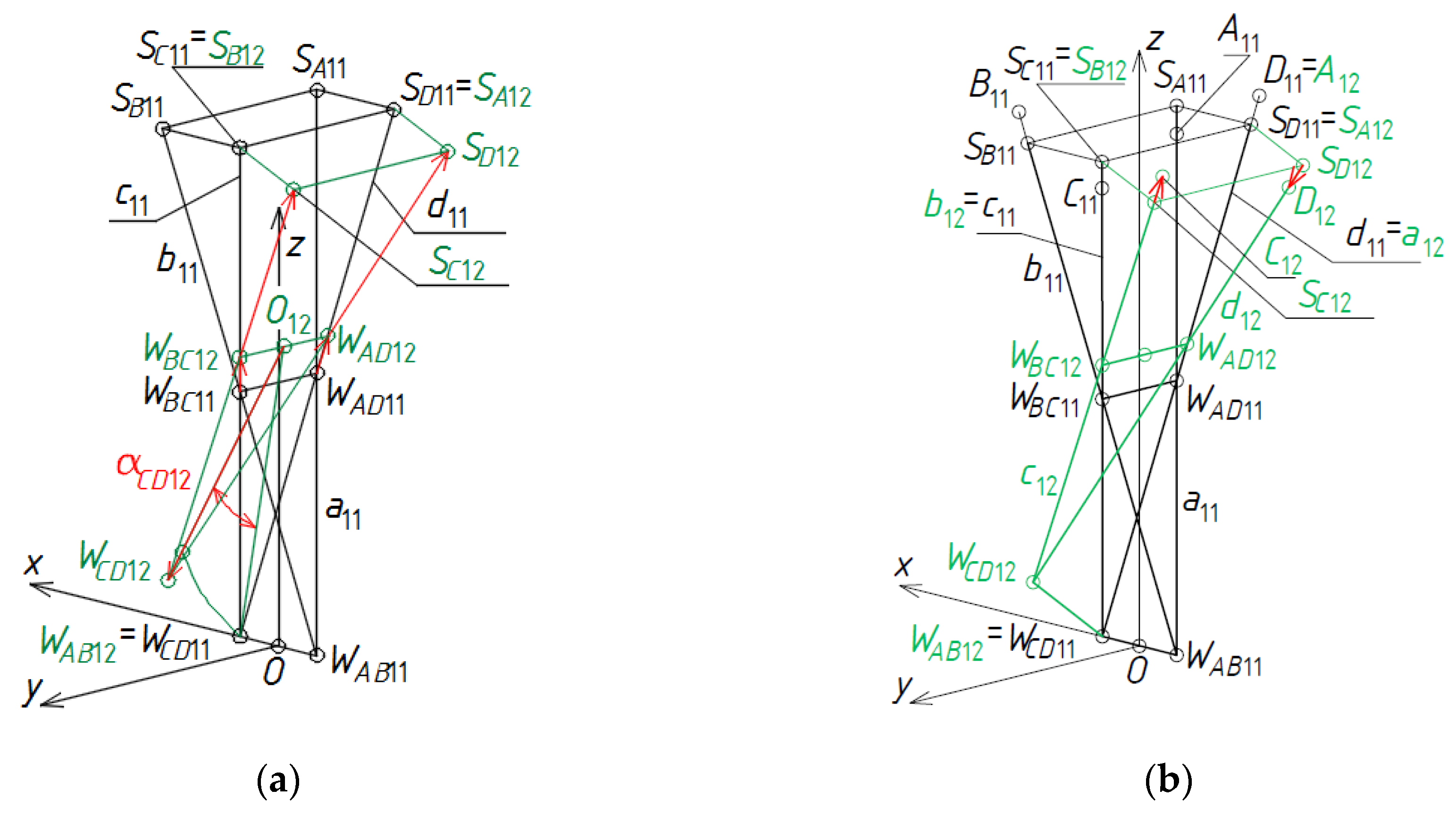
The second step of the algorithm relates to the determination of the reference tetrahedron Γ₁₂, Figure 20a,b. At first, a second set of initial data must be adopted. The set is composed of the measures of the angles and vectors employed in the algorithm to define the positions of all characteristic points of Γ₁₂.

Four vertices of Γ₁₂ are determined as follows. Vertex W_AB12 is identical with W_CD11 of Γ₁₁ introduced previously. Positions of the vertices W_BC12 = T_BC12(W_BC11), W_AD12 = T_AD12(W_AD11) are defined on two side edges b₁₂ = c₁₁, a₁₂ = d₁₁ so that the measures of the vectors W_AD11W_AD12 and W_BC11W_BC12 are elements of the second set of initial data. The position of vertex W_CD12 is obtained as a result of a composition of the rotation O_{WAD12_WBC12} of O₁₂W_AB11 about the axis W_AD12W_BC12 by the angle α_CD12 and the translation T_CD12 of O₁₂ by the vector O₁₂W_CD12, where O₁₂ is a point of the (W_AD12, W_BC12) straight line. If the reference tetrahedron Γ₁₂ is to be symmetrical about the z-axis, W_BC12 and W_AD12 have to be symmetric to each other towards the (x,z)-plane and O₁₂ has to be the middle point of the edge W_BC12W_AD12. Four vertices W_AB12, W_CD12, W_AD12, and W_BC12 determine four straight side edges: a₁₂, b₁₂, c₁₂, and d₁₂ of Γ₁₂.

Four auxiliary points belonging to a reference surface ω_r and Γ are constructed so that S_A12 = S_D11, S_B12 = S_C11, S_C12 = T_SC12(W_BC12), S_D12 = T_SD12(W_AD12), where the measures of the vectors W_BC12S_C12 and W_AD12S_D12 are two elements of the second set of initial data. On the basis of two other elements of the second set, four points A₁₂ = D₁₁, B₁₂ = C₁₁, C₁₂ = T_C12(S_C12), D₁₂ = T_D12(S_D12), Figure 20b, constituting the vertices of a closed spatial quadrilateral line modeling shell roof eaves are constructed.

The third step of the method’s algorithm relates to determination of the reference tetrahedron Γ₂₁, Figure 21a,b. The third set of initial data, composed of the measures of the respective angles and vectors employed to define all specific points of Γ₂₁ is adopted.

Four vertices W_AB21, W_CD21, W_AD21, and W_BC21 of Γ₂₁ are determined as follows, Figure 21a. The vertex W_AD21 = W_BC11. The positions of vertices W_AB21 = T_AB21(W_AB11), W_CD21 = T_CD21(W_CD11) are defined on two side edges a₂₁ = b₁₁, d₂₁ = c₁₁, Figure 21b, so that the measures of the vectors W_AB11W_AB21 and W_CD11W_CD21 are two elements of the third set of initial data. The position of W_BC21 = T_BC21O_{WCD21_WAB21}(W_BC11) is obtained as a result of a composition of the rotation O_{WCD21_WAB21} of O₂₁W_AD21 about the axis W_CD21W_AB21 by the angle α_BC21 and the translation T_BC21 of O₂₁ by the vector O₂₁W_BC21, where O₂₁ is a point of the straight line W_CD21W_AB21. If the reference tetrahedron Γ₂₁ is to be symmetrical towards the (y,z)-plane, the positions of points W_CD21 and W_AB21 have to be symmetric to each other towards the (y,z)-plane and O₂₁ has to be the middle point of the segment W_CD21W_AB21. Four vertices W_AB21, W_CD21, W_AD21, and W_BC21 determine four straight side edges: a₂₁, b₂₁, c₂₁ and d₂₁ of Γ₂₁.

Four auxiliary points belonging to ω_r are determined on the side edges of Γ₂₁ so that S_A21 = S_B11, S_D21 = S_C11, S_C21 = T_SC21(W_BC21) and S_B21 = T_SB21(W_BC21), where the measures of the vectors W_BC21S_C21 and W_BC21S_B21 belong to the third set of initial data.

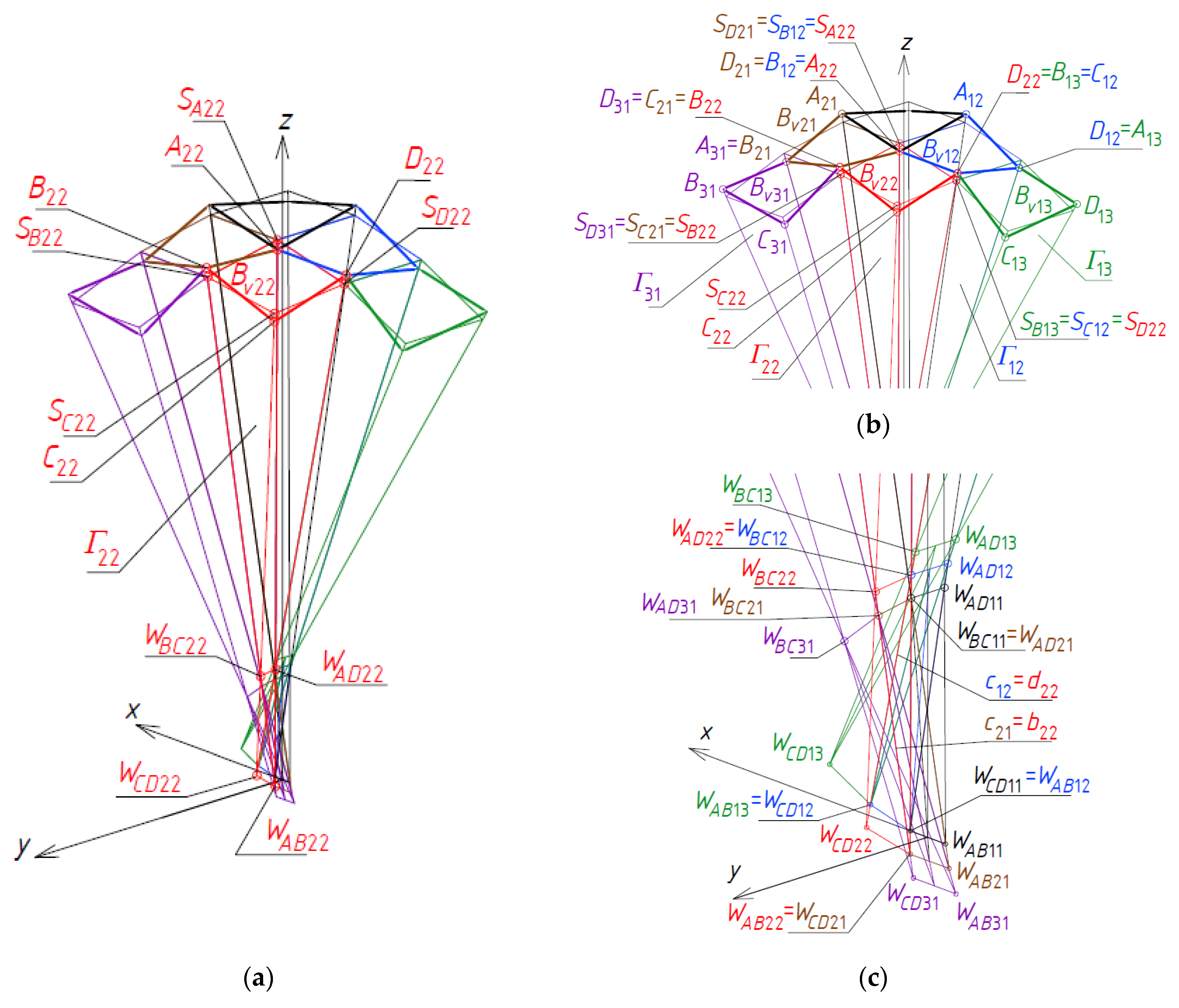
The fourth step of the method’s algorithm concerns a determination of the reference tetrahedron Γ₂₂, Figure 22a,b. The fourth set composed of the measures of the vectors and angles employed in this step is adopted.

Four vertices W_AD22 = W_BC12, W_AB22 = W_CD21, W_BC22 = T_BC22(W_BC21), W_CD22 = T_CD22(W_CD12) of Γ₁₂, Figure 22a, are defined so that the measures of the vectors W_BC21W_BC22 and W_CD21W_CD22 are two elements of the fourth set of initial data. Four vertices W_AB22, W_CD22, W_AD22, and W_BC22 determine four straight side edges: a₂₂, b₂₂, c₂₂, and d₂₂ and two axes u₂₂ and v₂₂ of Γ₂₂ Figure 23a.

Four auxiliary points of Γ belonging to ω_r are constructed so that S_A22 = S_C11, S_D22 = S_C12, S_B22 = S_C21, and S_C22 = T_C22(W_BC22), Figure 23b, where the measure of the vector W_BC22S_C22 is a value belonging to the fourth set of the initial data. On the basis of these points of ω_r, four points A₂₂ = C₁₁, B₂₂ = C₂₁, C₂₂ = T_C22(S_C22), D₂₂ = C₁₂ constituting the vertices of a closed spatial quadrilateral line modeling complete shell roof eaves are constructed.

The result of adding up the four reference tetrahedrons Γ_ij constructed above is a subnet Γ₁ constituting about one-fourth of the designed reference network Γ. The other three parts of Γ can be built using z-axis symmetry and two (x,z)- and (y,z)-plane symmetries called 3D-mirrors, Figure 24a,b, in the way described Section 6 with the help of a certain example. All obtained points S_Aij, S_Bij, S_Cij, and S_Dij, Figure 24a, and their images obtained as a result of the aforementioned symmetries are the selected vertices of a certain net defining ω_r, Figure 24b. In relation to this net, a roof structure Ω composed of nine sectors Ω_ij is positioned. Thus, the vertices of the eaves of each Ω_ij segment of the roof structure Ω are defined on the basis of ω_r, Figure 25.

In addition, it is worth paying attention to the following properties of the reference network Γ built so far. The vertices of each reference tetrahedron Γ_ij designate side edges a_ij, b_ij, c_ij, and d_ij and planes of Γ. Each new reference tetrahedron Γ_i+1j or Γ_ij+1 is created as a spatial mesh having four sought-after vertices defined in the selected side edges of the previously constructed tetrahedrons Γ_ij to obtain subsequent pairs of the adjacent meshes having common planes. In the aforementioned planes of Γ, the locations of roof directrices are determined.

In the case of creating a reference tetrahedron contained in any of the two orthogonal directions related to the first z-axially symmetrical tetrahedron Γ₁₁, one its vertex is laid outside the side edges of the already created subnet of Γ. This vertex determines a new plane of Γ passing through the already constructed axis of this tetrahedron. However, in the case of two directions diagonal in relation to the first Γ₁₁, each new reference tetrahedron has to have two vertices identical to two from the four previously constructed vertices of Γ and two other new vertices have to be determined on two side edges of the previously created subnet of Γ.

This way of constructing the subsequent reference tetrahedrons located in these orthogonal and diagonal directions leads to the fact that each inner side edge of Γ is shared by four adjacent reference tetrahedrons and eight vertices of these four tetrahedrons belong to this side edge. In a general case, these vertices occupy four different positions, in pairs.

Therefore, it seems rational to carry out a process of a geometric parameterization of this type of reference networks, especially the mutual positions of their vertices and other characteristic points. An example of using such an algorithm for a parametric determination of reference polyhedral networks Γ and eaves nets B_v is given in Section 6, where certain division coefficients of the selected pairs of some adjacent vertices by other vertices of the reference network are employed. In addition, some points belonging to a reference surface and vertices of the eaves edge line of each individual roof shell segment are defined at each side edge of the network Γ. It is also advisable to use analogous division coefficients of pairs of the reference network’s vertices in determining these points of the reference surface and the eaves limiting the individual roof shell segments. An example of making such a parameterization is included in Section 6.

6. Parametric Shaping of an Example Reference Network and a Free Form Shell Roof

The algorithm assisted computationally leads to creation of intuitive engineering parametric and regular models of attractive and rational building free forms. To create such models stiff motions including translations and rotations of points and planes presented in the previous section are going to be replaced by slightly more complex actions related to the division coefficients and proportions of some elements of the reference Γ and eaves B_v networks. These coefficients and proportions allow us to define the positions of (1) the sought-after vertices of Γ with respect to the adopted or calculated at one of the previous steps pairs of other vertices of Γ, (2) the subsequent planes of Γ, (3) the points S_Air, S_Bij, S_Cij, and S_Dij belonging to a reference surface w_r, (4) the vertices A_ij B_ij, C_ij and D_ij of B_v relative to the already determined vertices of Γ and these points of w_r.

A use of the method for determining a quarter Γ₁ of a reference network Γ, Figure 26, and a quarter B_v1 of B_v consisting of closed spatial quadrangles B_vij, is presented below. It is based on some adopted proportions. All vertices of the other three quarters Γ_2L, Γ_3p, Γ_4r of Γ, Figure 26, and B_v2L, B_v3p, B_v4r of B_v are determined using: (1) a z-axial symmetry, in the case of Γ_2L, (2) a (x,z)-plane symmetry called 3D-mirror, where Γ_3p is constructed, (3) a (y,z)―plane symmetry for Γ_4r.

Creating the z-axially symmetric network Γ is started with defining the first z-axially symmetric mesh Γ₁₁, Figure 27. The subsequent meshes Γ_ij are determined in the order presented in the previous section, Figure 18, Figure 19, Figure 20, Figure 21, Figure 22, Figure 23, Figure 24 and Figure 25. In order to build the mesh Γ₁₁, the following quantities and proportions are adopted. The values of these variables are given in

Table 1. The initial data defining the shapes of the meshes Γ₁₁ and B_v11 of Γ and B_v.

Variable or Division Coefficient	Value	Unit
α11	10.0
WAB11WCD11	2000.0	mm
OWBC11	100,00.0	mm
dOW11	1.0	-
dS11	2.5	-
dd11	0.1	-

.

Two opposite planes (W_AB11, W_CD11, W_BC11) and (W_AB11, W_CD11, W_AD11), Figure 27a–c, are inclined to each other at an angle α₁₁ = 2 α_BC11 = 2 α_AD11, Figure 19. The length of the edge W_CD11W_AB11 contained in the u₁-axis was adopted in accordance with the values given in Table 1.

The W_BC11W_AD11’s length results from the adopted values of the angle α₁₁ and the height OW_BC11 of the triangle <W_AB11, W_CD11, W_BC11> as well as the proportion.

d_OW11= OW_AD11/OW_BC11

The positions of points S_A11, S_V11, S_C11, and S_D11 are defined with the same constant d_S11 listed in Table 1 as follows

$${\mathrm{d}}_{SA11}=m(\overrightarrow{W_{AB11}{S}_{A11}})/m(\overrightarrow{W_{AB11}{W}_{AD11}})$$

$${\mathrm{d}}_{SB11}=m(\overrightarrow{W_{AB11}{S}_{B11}})/m(\overrightarrow{W_{AB11}{W}_{BC11}})$$

$${\mathrm{d}}_{SC11}=m(\overrightarrow{W_{CD11}{S}_{C11}})/m(\overrightarrow{W_{CD11}{W}_{BC11}})$$

$${\mathrm{d}}_{SD11}=m(\overrightarrow{W_{CD11}{S}_{D11}})/m(\overrightarrow{W_{CD11}{W}_{AD11}})$$

d_SB11 = d_SA11 = d_SC11 = d_SD11 = d_S11

where $\overrightarrow{W_{AB11}{W}_{AD11}}$ is the vector starting with W_AB11 and ending at W_AD11, m($\overrightarrow{W_{AB11}{W}_{AD11}}$) is the measure of $\overrightarrow{W_{AB11}{W}_{AD11}}$, $\overrightarrow{W_{AB11}{S}_{A11}}$ is the vector whose starting point is W_AB11 and ending point is S_A11, etc. Thus, the location of points S_A11, S_B11, S_C11 and S_D11 is defined on the basis of the adopted division coefficients of all pairs {W_AB11, W_AD11}, {W_AB11, W_BC11}, {W_CD11, W_BC11} and {W_CD11, W_AD11} of the vertices of the Γ₁₁ mesh. The subsequent four points S_A11, S_B11, S_C11 and S_D11 usually form a flat rectangle determining the reference surface ω_r in relation to which the shell segments of the designed multi-segment shell roof are arranged in the three-dimensional space.

The locations of the vertices A₁₁, B₁₁, C₁₁ and D₁₁ of Γ₁₁, Figure 27a, are defined by means of the following proportions

$${\mathrm{d}}_{A11}=m(\overrightarrow{W_{AB11}{A}_{11}})/m(\overrightarrow{W_{AB11}{W}_{AD11}})$$

$${\mathrm{d}}_{B11}=m(\overrightarrow{W_{AB11}{B}_{11}})/m(\overrightarrow{W_{AB11}{W}_{BC11}})$$

$${\mathrm{d}}_{C11}=m(\overrightarrow{W_{CD11}{C}_{11}})/m(\overrightarrow{W_{CD11}{W}_{BC11}})$$

$${\mathrm{d}}_{D11}=m(\overrightarrow{W_{CD11}{D}_{11}})/m(\overrightarrow{W_{CD11}{W}_{AD11}})$$

where $\overrightarrow{W_{AB11}{A}_{11}}$ is the vector having the starting point at W_AB11 and the end point at A₁₁, etc. Points A₁₁, B₁₁, C₁₁, and D₁₁ determine a spatial quadrangle B_v11 constituting the eaves of a single, smooth, shell segment Ω₁₁ modeling a single shell of a complex roof structure. It was adopted a constant dd₁₁ to calculate the values of four division coefficients d_A11, d_B11, d_C11, and d_D11. This constant is used with positive or negative sign depending on whether the points A₁₁, B₁₁, C₁₁, and D₁₁ lie above or below ω_r defined in the corresponding area by means of the quadrangle S_A11S_B11S_C11S_D11, Figure 27a. The ratios d_A11, d_B11, d_C11, and d_D11 are calculated as follows

d_A11 = d_SA11 + dd_A11

d_B11 = d_SB11 + dd_B11

d_C11 = d_SC11 + dd_C11

d_D11 = d_SD11 + dd_D11

dd_B11 = −dd_A11 = −dd_C11 = dd_D11 = dd₁₁

In order to construct Γ₁₂, Figure 27b, the values presented in

Table 2. The initial data defining the shapes of Γ₁₂ and B_v12.

Division Coefficient	Value
dαCD12	1.2
dO12WCD12	1.0
dWBC12, dWAD12	1.1
dSC12, dSD12	2.5
dd12	0.1

were adopted.

The angle α_CD12 is defined by means of the angle α₁₁ adopted in the previous step and the following formula.

dα_CD12 = α_CD12/α₁₁

In order to determine W_CD12, it was also adopted the following relationship

$${\mathrm{d}}_{O12WCD12}=m(\overrightarrow{O_{12}{W}_{CD12}})/m(\overrightarrow{O_{12}{W}_{AB12}})$$

where O₁₂ is the middle of the segment W_AD12W_BC12. The aforementioned values are listed in Table 2. Two new division coefficients d_WBC12 and d_WAD12 are adopted as follows

$${\mathrm{d}}_{WBC12}=m(\overrightarrow{W_{CD11}{W}_{BC12}})/m(\overrightarrow{W_{CD11}{W}_{BC11}})$$

$${\mathrm{d}}_{WAD12}=m(\overrightarrow{W_{CD11}{W}_{AD12}})/m(\overrightarrow{W_{CD11}{W}_{AD11}})$$

where m($\overrightarrow{W_{CD11}{W}_{BC12}}$) is the measure of the vector $\overrightarrow{W_{CD11}{W}_{BC12}}$ having the starting point at W_CD11 and the end point at W_BC12, and m($\overrightarrow{W_{CD11}{W}_{BC11}}$) is the measure of the vector $\overrightarrow{W_{CD11}{W}_{BC11}}$, etc.

The positions of points S_A12 and S_B12 are similar to the positions of S_D11 and S_C11 determined previously for Γ₁₁. The positions of S_C12 and S_D12 result from the following proportions

d_SC12 = d_SD12 = d_S11

The assumed values of these proportions are given in Table 2. The positions of points A₁₂ = D₁₁, B₁₂ = C₁₁ are calculated previously for Γ₁₁. The positions of points C₁₂ and D₁₂ can determined by means of the following proportions

d_C12 = d_SC12 + dd_C12

d_D12 = d_SD12 + dd_D12

dd_C12 = −dd_D12 = dd₁₂ = dd₁₁

where the considered values are listed in Table 2.

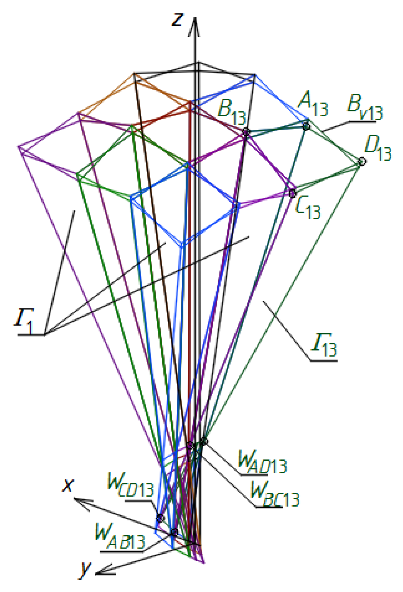
The sought-after vertices W_AB13, W_AD13, W_CD13, and W_BC13 of Γ₁₃ constituting one mesh of Γ₁, Figure 28a, the points S_A13, S_B13, S_C13, and S_D13 of ω_r and the vertices A₁₃, B₁₃, C₁₃, and D₁₃ of the closed eaves quadrangle B_v13, Figure 28b, can be defined analogously as for Γ₁₂ and B_v12 using the following formula

dα_CD13 = α_CD13/α₁₁

$${\mathrm{d}}_{O13WCD13}=m(\overrightarrow{O_{13}{W}_{CD13}})/m(\overrightarrow{O_{13}{W}_{AB13}})$$

$${\mathrm{d}}_{WBC13}=m(\overrightarrow{W_{CD12}{W}_{BC13}})/m(\overrightarrow{W_{CD12}{W}_{BC12}})$$

$${\mathrm{d}}_{WAD13}=m(\overrightarrow{W_{CD12}{W}_{AD13}})/m(\overrightarrow{W_{CD12}{W}_{AD12}})$$

d_SC13 = d_SD13 = d_S11

d_C13 = d_SC13 + dd_C13

d_D13 = d_SD13 + dd_D13

dd_D13 = −dd_C13 = dd₁₃ = dd₁₁

where O₁₃ is the middle point of W_AD13W_BC13.

The mutual position of the adjacent meshes B_v12 and B_v13 results from the relationships adopted for all meshes of B_v, which are as follows S_A13 = S_D12, S_B13 = S_C12, A₁₃ = D₁₂, B₁₃ = C₁₂, Figure 28a. The values of the adopted new proportions are given in

Table 3. The initial data defining the shapes of the meshes Γ₁₃ and B_v13 of Γ and B_v.

Division Coefficient	Value
dαCD13	1.2
dO13WCD13	1.0
dWBC13, dWAD13	1.1
dSC13, dSD13	2.5
dd13	0.1

.

Compared to the investigated way for creating Γ_1j and B_v1j meshes (for j = 1 to 3) of the first orthogonal direction in Γ, the manner of determining the subsequent Γ_i1 and B_vi1 meshes (for i = 1 to 3) of the second orthogonal direction in Γ, Figure 29a, needs a slight modification.

The angle α_BC21 is a function of the angle α₁₁, defined with the help of the following formula

dα_BC21 = α _BC21/α₁₁

The following relations were adopted

$${\mathrm{d}}_{O21WBC21}=m(\overrightarrow{O_{21}{W}_{BC21}})/m(\overrightarrow{O_{21}{W}_{BC11}})$$

$${\mathrm{d}}_{WCD21}=m(\overrightarrow{W_{BC11}{W}_{CD21}})/m(\overrightarrow{W_{BC11}{W}_{CD11}})$$

$${\mathrm{d}}_{WAB21}=m(\overrightarrow{W_{AD11}{W}_{CD21}})/m(\overrightarrow{W_{AD11}{W}_{CD11}})$$

where O₂₁ is the middle point of the edge W_CD21W_AB21, Figure 29b. The positions of points S_A21 and S_D21 are similar to the positions of points S_B11 and S_C11 obtained previously for Γ₁₁. The positions of points S_B21 and S_C21, Figure 29a, result from adopting of the following proportions

d_SB21 = d_SC21 = d_S11

$${\mathrm{d}}_{SB21}=m(\overrightarrow{W_{AB21}{S}_{B21}})/m(\overrightarrow{W_{AB211}{W}_{BC21}})$$

$${\mathrm{d}}_{SC21}=m(\overrightarrow{W_{CD21}{S}_{C21}})/m(\overrightarrow{W_{CD21}{W}_{BC21}})$$

whose values are given in

Table 4. The initial data defining the meshes Γ₂₁ and B_v21.

Division Coefficient	Value
dαCD21	1.2
dO21WBC21	1.0
dWCD21, dWAB21	1.1
dSB21, dSC21	2.5
dd21	0.1

. The positions of points A₂₁ = B₁₁ and D₂₁ = C₁₁. The positions of the points B₂₁ and C₂₁ result from adopting of the following proportions

d_B21 = d_SB21 + dd_B21

d_C21 = d_SC21 + dd_C21

dd_C21 = −dd_B21 = dd₂₁ = dd₁₁

To create Γ₂₁ and B_v21, Figure 29a, the values listed in Table 4 are employed.

All vertices W_AB31, W_AD31, W_CD31 and W_BC31 of Γ₃₁, four points S_A31, S_B31, S_C31, and S_D31 of ω_r and all vertices A₃₁, B₃₁, C₃₁, and D₃₁ of B_v31 are determined like for Γ₂₁, Figure 30a,b. For this purpose, the following proportions are defined

dα_BC31 = α _BC31/α _BC21

$${\mathrm{d}}_{O31WBC31}=m(\overrightarrow{O_{31}{W}_{BC31}})/m(\overrightarrow{O_{31}{W}_{BC21}})$$

$${\mathrm{d}}_{WCD31}=m(\overrightarrow{W_{BC21}{W}_{CD31}})/m(\overrightarrow{W_{BC21}{W}_{CD21}})$$

$${\mathrm{d}}_{WAB31}=m(\overrightarrow{W_{AD21}{W}_{CD31}})/m(\overrightarrow{W_{AD21}{W}_{CD21}})$$

d_SB31 = d_SC31 = d_S11

$${\mathrm{d}}_{SB31}=m(\overrightarrow{W_{AB31}{S}_{B31}})/m(\overrightarrow{W_{AB231}{W}_{BC31}})$$

$${\mathrm{d}}_{SC31}=m(\overrightarrow{W_{CD31}{S}_{C31}})/m(\overrightarrow{W_{CD31}{W}_{BC31}})$$

d_B31 = d_SB31 + dd_B31

d_C31 = d_SC31 + dd_C31

dd_B31 = −dd_C31 = dd₃₁ = dd₂₁

where O₃₁ is the middle point of W_CD31W_AB31. The locations of points S_A31 = S_B21, S_D31 = S_C21, A₃₁ = B₂₁, and D₃₁ = C₂₁. All values of the proportions defined above are shown in

Table 5. The initial data defining the meshes Γ₃₁ and B_v31.

Division Coefficient	Value
dαCD31	1.0
dO31WBC31	1.0
dWCD31, dWAB31	1.1
dSB31, dSC31	2.5
dd31	0.1

.

To create the tetrahedron Γ₂₂ and the quadrangle B_v22, Figure 31a, the values listed in

Table 6. The initial data defining the shapes of the meshes Γ₂₂ and B_v22.

Division Coefficient	Value
dWCD22	1.0
dWBC22	1.0
dSC22	2.5
dd21	−0.1

are adopted. To determine the position of W_CD22 on the straight line c₂₂, Figure 31a,c, a coefficient d_WCD22 defining the division of the edge W_BC12W_CD12 by the point W_CD22 is defined as follows

$${\mathrm{d}}_{WCD22}=m(\overrightarrow{W_{BC12}{W}_{CD22}})/m(\overrightarrow{W_{BC12}{W}_{CD12}})$$

To determine the location of W_BC22 on b₂₂ = c₂₁, a coefficient d_WBC22 defining the division of the edge W_CD21W_BC21 by the point W_BC22 is assumed, Figure 31c, so that

$${\mathrm{d}}_{WBC22}=m(\overrightarrow{W_{CD12}{W}_{BC22}})/m(\overrightarrow{W_{CD21}{W}_{BC21}})$$

In addition, W_AB22 = W_CD21, W_AD22 = W_BC12. Similarly, the values of two coefficients d_SC22 and dd_C22 are adopted. The first value defines a division ratio of the edge W_CD22W_BC22 by S_C22, Figure 31c,

$${\mathrm{d}}_{SC22}=m(\overrightarrow{W_{CD22}{S}_{C22}})/m(\overrightarrow{W_{CD22}{W}_{BC22}})$$

The second proportion together with the first one enables one to define a division ratio of the edge W_CD22W_BC22 by C₂₂

$${\mathrm{dd}}_{SC22}=m(\overrightarrow{W_{CD22}{C}_{22}})/m(\overrightarrow{W_{CD22}{W}_{BC22}})$$

where

d_C22 = d_SC22 + dd_SC22

Analogous proportions as for Γ₂₂ positioned diagonally towards Γ₁₁ are defined for: (1) Γ₂₃ and Γ₃₂, located diagonally in relation to Γ₁₂ and Γ₂₂. (2) Γ₃₃ located diagonally towards Γ₂₂. Values of these proportions are listed in

Table 7. The initial data defining the meshes Γ₂₃, Γ₃₂, Γ₃₃ and B_v23, B_v32, B_v33.

Division Coefficient	Value
dWCD23	1.0
dWBC23	1.0
dSC23	2.5
ddC23	0.1
dWCD32	1.0
dWBC32	1.0
dSC32	2.5
ddC32	0.1
dWCD33	1.0
dWBC233	1.0
dSC233	2.5
ddC33	−0.1

. A sum of all Γ_ij (for i = 1–3) achieved so far is a subnet Γ₁ constituting about one quarter of Γ. It is contained in the dihedral angle limited by the planes (x,z) and (y,z) containing the positive y-axis and negative x-axis, Figure 32.

The reference tetrahedrons Γ_1j and Γ_i1 for (for i, j = 1 to 3) of the subnet Γ₁ were arranged in two orthogonal directions along the principal planes (x,z) and (y,z) of [x,y,z]. However, other tetrahedrons Γ_ij (for i, j = 2 to 3) are arranged in diagonal directions towards the Γ₁₁ mesh. To construct these tetrahedrons, a relatively small number of the respective proportions is employed.

The calculated coordinates of all vertices of the subnets Γ₁ and B_v1 are given in

Table A1. The coordinates of the vertices W_ABij, W_CDij, W_ADij, W_BCij (for i, j = 1, 2, 3) of the polyhedral reference network Γ₁ shown in Figure 27.

Point	x-Coordinate [mm]	y-Coordinate [mm]	z-Coordinate [mm]
WAB11	4500.0	−4793.6	54,790.7
WCD11	4500.0	4880.7	55,786.9
WAD11	−4500.0	4793.6	54,790.7
WBC11	−4500.0	−4880.7	55,786.9
WAB12	xWCD11	yWCD11	zWCD11
WCD12	3254.3	0.0	468.2
WAD12	−100.0	−958.7	10,958.1
WBC12	−100.0	958.7	10,958.1
WAB13	xWCD12	yWCD12	zWCD12
WCD13	5572.7	0.0	zSC12
WAD13	−435.4	−1054.6	12,007.1
WBC13	−435.4	1054.6	12,007.1
WAB21	−1100.0	−87.2	−996.2
WCD21	1100.0	−87.2	−996.2
WAD21	xWBC11	yWBC11	zWBC11
WBC21	0.0	2574.0	9677.1
WAB31	−1210.0	−353.3	−2063.5
WCD31	1210.0	353.3	−2063.5
WAD31	−xWBC21	yWBC21	zWBC21
WBC31	0.0	4374.6	9074.6
WAB22	xWCD21	yWCD21	zWCD21
WCD22	3589.7	0.0	−580.8
WAD22	xWBC12	yWBC12	zWBC12
WBC22	−110.0	2840.1	10,744.4
WAB23	xWCD22	yWCD22	zWCD22
WCD23	6173.6	−105.5	435.5
WAD23	xWBC13	yWBC13	zWBC13
WBC23	−480.0	3133.7	11,876.9
WAB32	xWCD31	yWCD31	zWCD31
WCD32	3959.7	−389.5	−1713.3
WAD32	xWBC22	yWBC22	zWBC22
WBC32	−121.0	4847.4	10,188.4
WAB33	xWCD32	yWCD32	zWCD32
WCD33	6838.9	−429.4	−708.6
WAD33	xWBC23	yWBC23	zWBC23
WBC33	−529.1	5371.0	11,378.6

,

Table A2. The coordinates of the points S_Aij, S_Bij, S_Cij, S_Dij for (i,j = 1, 2, 3) of the reference surface ω_r.

Point	x-Coordinate [mm]	y-Coordinate [mm]	z-Coordinate [mm]
SA11	4500.0	−4793.6	54,790.7
SB11	4500.0	4880.7	55,786.9
SC11	−4500.0	4793.6	54,790.7
SD11	−4500.0	−4880.7	55,786.9
SA12	xSD11	ySD11	zSD11
SB12	xSC11	ySC11	zSC11
SC12	−13,517.1	4793.6	52,918.0
SD12	−13,517.1	−4793.6	52,918.0
SA13	xSD12	ySD12	zSD12
SB13	xSC12	ySC12	zSC12
SC13	−21,737.1	4793.6	49,304.2
SD13	−21,737.1	−4793.6	49,304.2
SA21	xSB11	ySB11	zSB11
SB21	4500.0	13,460.5	53,340.4
SC21	−4500.0	13,460.5	53,340.4
SD21	xSC11	ySC11	zSC11
SA31	xSB21	ySB21	zSB21
SB31	4500.0	21,957.5	50,497.3
SC31	−4500.0	21,957.5	50,497.3
SD31	xSC21	ySC21	zSC21
SA22	xSC11	ySC11	zSC11
SB22	xSC21	ySC21	zSC21
SC22	−13,675.6	13,605.3	52,270.2
SD22	xSC12	ySC12	zSC12
SA23	xSC12	ySC12	zSC12
SB23	xSC22	ySC22	zSC22
SC23	−22,104.0	13,660.9	49,061.5
SD23	xSC13	ySC13	zSC13
SA32	xSC21	ySC21	zSC21
SB32	xSC31	ySC31	zSC31
SC32	−13,692.4	22,263.8	49,770.7
SD32	xSC22	ySC22	zSC22
SA33	xSC22	ySC22	zSC22
SB33	xSC32	ySC32	zSC32
SC33	−22,428.4	22,611.2	47,304.5
SD33	xSC23	ySC23	zSC23

and

Table A3. The coordinates of the vertices A_ij, B_ij, C_ij, D_ij (for i, j = 1, 2, 3) of the eaves edge net B_v1.

Point	x-Coordinate [mm]	y-Coordinate [mm]	z-Coordinate [mm]
A11	4,400.0	−4,706.4	53,794.5
B11	4,600.0	4,880.7	55,786.9
C11	−4,400.0	4,706.4	53,794.5
D11	−4,600.0	−4,880.7	55,786.9
A12	−4,390.0	−4,697.7	53,694.9
B12	−4,610.0	4,889.4	55,886.5
C12	−13,517.1	4,697.9	51,869.0
D12	−13,852.6	−4,889.4	53,967.0
A13	−13,148.2	−4,688.1	51,764.1
B13	−13,886.1	4,899.0	54,071.9
C13	−21,136.3	4,688.1	48,252.2
D13	−22,338.0	−4,899.0	50,356.2
A21	4,390.0	4,697.7	53,694.9
B21	4,610.0	13,726.6	54,407.7
C21	−4,390.0	13,194.4	52,273.0
D21	xB12	yB12	zB12
A31	4,379.0	13,167.7	52,166.3
B31	4,621.0	22,430.3	51611.1
C31	−4,379.0	21,484.7	49,383.5
D31	−4,621.0	13,753.2	54,514.4
A22	xC11	yC11	zC11
B22	xD31	yD31	zD31
C22	−13,367.3	13,360.7	51,326.4
D22	xB13	yB13	zB13
A23	xC12	yC12	zC12
B23	−13,983.9	13,850.0	53,213.9
C23	−21,549.5	13,391.0	48,108.1
D23	−22,338.0	4,899.0	50,356.2
A32	xC21	yC21	zC21
B32	−4,621.0	22,430.3	51,611.1
C32	−13,352.3	21,827.4	48,778.9
D32	xB23	yB23	zB23
A33	xC22	yC22	zC22
B33	−14,032.4	22,700.2	50,762.6
C33	−21,916.7	22,208.4	46,465.1
D33	−22,658.4	13,930.9	50,015.0

posted in Appendix A. Table A1 applies to all vertices W_ABij, W_CDij, W_ADij, and W_BCij of Γ₁ (for i, j = 1 to 3). Table A2 relates to the vertices S_Aij, S_Bij, S_Cij, and S_Dij of ω_r. Table A3 concerns all vertices A_ij, B_ij, C_ij, and D_ij of B_v1.

In order to create the second pair of subnets Γ_2L and B_v2L of Γ and B_v, the z-axis-symmetry of all characteristic points W_ABij, W_CDij, W_ADij, W_BCij, A_ij, B_ij, C_ij, D_ij, S_Aij, S_Bij, S_Cij, and S_Dij of the previously constructed subnets Γ₁ and B_v1 is used. As a result of this transformation, the vertices W_ABijL, W_CDijL, W_ADijL and W_BCijL of Γ_2L, the vertices A_ijL, B_ijL, C_ijL, and D_ijL of B_vijL as well as the points S_AijL, S_BijL, S_CijL, and S_DijL of ω_r are determined so that S_AijL, S_BijL, S_CijL, S_DijL, A_ijL, B_ijL, C_ijL, and D_ijL belong to the dihedral angle located between the (x,z)-plane and (y,z)-plane and including the positive x-half-axis and the negative y-half-axis, Figure 33. Examples of a single reference tetrahedron Γ_13L of the subnet Γ_2L and a mesh B_v13L of the subnet B_v2L are shown in Figure 33.

For the subnets Γ_2L and B_v2L, there are many proportions between the lengths of their side edges and axes and the measures of their angles, identical to those obtained for Γ₁ and B_v1. Some selected relations resulting from the z-axis-symmetry of the vertices of Γ_2L and B_v2L and the corresponding vertices of Γ₁ and B_v1 are listed in

Table A4. The coordinates of the vertices W_ABijL, W_CDijL, W_ADijL, W_BCijL (for i, j = 1, 2, 3) of the polyhedral reference network Γ_2L shown in Figure 28.

Vertex	x-Coordinate [mm]	y-Coordinate [mm]	z-Coordinate [mm]
WAB12L	−xWCD12	−yWCD12	zWCD12
WCD12L	xWAB11	yWAB11	zWAB11
WAD12L	−xWBC12	−yWBC12	zWBC12
WBC12L	−xWAD12	−yWAD12	zWAD12
WAB13L	−xWCD13	−yWCD13	zWCD13
WCD13L	xWAB12 L	yWAB12 L	zWAB12 L
WAD13L	−xWBC13	−yWBC13	zWBC13
WBC13L	−xWAD13	−yWAD13	zWAD13
WAB21L	−xWCD21	−yWCD21	zWCD21
WCD21L	−xWAB21	−yWAB21	zWAB21
WAD21L	−xWBC21	−yWBC21	zWBC21
WBC21L	−xWAD21	−yWAD21	zWAD21
WAB31L	−xWCD31	−yWCD31	zWCD31
WCD31L	−xWAB31	−yWAB31	zWAB31
WAD31L	−xWBC31	−yWBC31	zWBC31
WBC31L	−xWAD31	−yWAD31	zWAD31
WAB22L	−xWCD22	−yWCD22	zWCD22
WCD22L	−xWAB22	−yWAB22	zWAB22
WAD22L	−xWBC22	−yWBC22	zWBC22
WBC22L	−xWAD22	−yWAD22	zWAD22
WAB23L	−xWCD23	−yWCD23	zWCD23
WCD23L	−xWAB23	−yWAB23	zWAB23
WAD23L	−xWBC23	−yWBC23	zWBC23
WBC23L	−xWAD23	−yWAD23	zWAD23
WAB32L	−xWCD32	−yWCD32	zWCD32
WCD32L	−xWAB32	−yWAB32	zWAB32
WAD32L	−xWBC32	−yWBC32	zWBC32
WBC32L	−xWAD32	−yWAD32	zWAD32
WAB33L	−xWCD33	−yWCD33	zWCD33
WCD33L	−xWAB3	−yWAB3	zWAB3
WAD33L	−xWBC33	−yWBC33	zWBC33
WBC33L	−xWAD33	−yWAD33	zWAD33

,

Table A5. The coordinates of the points S_AijL, S_BijL, S_CijL, S_DijL (for i, j = 1, 2, 3) of the reference surface ω_r.

Point	x-Coordinate [mm]	y-Coordinate [mm]	z-Coordinate [mm]
SA12L	−xSC12	−ySC12	zSC12
SB12L	−xSD12	−ySD12	zSD12
SC12L	−xSA12	−ySA12	zSA12
SD12L	−xSB12	−ySB12	zSB12
SA13L	−xSC12	−ySC13	zSC13
SB13L	−xSD13	−ySD13	zSD13
SC13L	−xSA13	−ySA13	zSA13
SD13L	−xSB13	−ySB13	zSB13
SA21L	−xSC21	−ySC21	zSC21
SB21L	−xSD21	−ySD21	zSD21
SC21L	−xSA21	−ySA21	zSA21
SD21L	−xSB21	−ySB21	zSB21
SA31L	−xSC31	−ySC31	zSC31
SB31L	−xSD31	−ySD31	zSD31
SC31L	−xSA31	−ySA31	zSA31
SD31L	−xSB31	−ySB31	zSB31
SA22L	−xSC22	−ySC22	zSC22
SB22L	−xSD22	−ySD22	zSD22
SC22L	−xSA22	−ySA22	zSA22
SD22L	−xSB22	−ySB22	zSB22
SA23L	−xSC23	−ySC23	zSC23
SB23L	−xSD23	−ySD23	zSD23
SC23L	−xSA23	−ySA23	zSA23
SD23L	−xSB23	−ySB23	zSB23
SA32L	−xSC32	−ySC32	zSC32
SB32L	−xSD32	−ySD32	zSD32
SC32L	−xSA32	−ySA32	zSA32
SD32L	−xSB32	−ySB32	zSB32
SA33L	−xSC33	−ySC33	zSC33
SB33L	−xSD33	−ySD33	zSD33
SC33L	−xSA33	−ySA33	zSA33
SD33L	−xSB33	−ySB33	zSB33

and

Table A6. The coordinates of the vertices A_ijL, B_ijL, C_ijL, D_ijL (for i, j = 1, 2, 3) of the eaves edge net B_v2L.

Point	x-Coordinate [mm]	y-Coordinate [mm]	z-Coordinate [mm]
A12L	−xC12	−yC12	zC12
B12L	−xD12	−yD12	zD12
C12L	−xA12	−yA12	zA12
D12L	−xB12	−yB12	zB12
A13L	−xC13	−yC13	zC13
B13L	−xD13	−yD13	zD13
C13L	−xA13	−yA13	zA13
D13L	−xB13	−yB13	zB13
A21L	−xC21	−yC21	zC21
B21L	−xD21	−yD21	zD21
C21L	−xA21	−yA21	zA21
D21L	−xB21	−yB21	zB21
A31L	−xC31	−yC31	zC31
B31L	−xD31	−yD31	zD31
C31L	−xA31	−yA31	zA31
D31L	−xB31	−yB31	zB31
A22L	−xC22	−yC22	zC22
B22L	−xD22	−yD22	zD22
C22L	−xA22	−yA22	zA22
D22L	−xB22	−yB22	zB22
A23L	−xC23	yC23	zC23
B23L	−xD23	−yD23	zD23
C23L	−xA23	−yA23	zA23
D23L	−xB23	−yB23	zB23
A32L	−xC32	−yC32	zC32
B32L	−xD32	−yD32	zD32
C32L	−xA32	−yA32	zA32
D32L	−xB32	−yB32	zB32
A33L	−xC33	−yC33	zC33
B33L	−xD33	−yD33	zD33
C33L	−xA33	−yA33	zA33
D33L	−xB330	−yB33	zB33

posted in Appendix A. Table A4 applies to the vertices W_ABijL, W_CDijL, W_ADijL, and W_BCijL of Γ_2L. Table A5 relates to the vertices S_AijL, S_BijL, S_CijL, and S_DijL of ω_r. Table A6 consists of the coordinates of the vertices A_ijL, B_ijL, C_ijL, and D_ijL belonging to B_v2L.

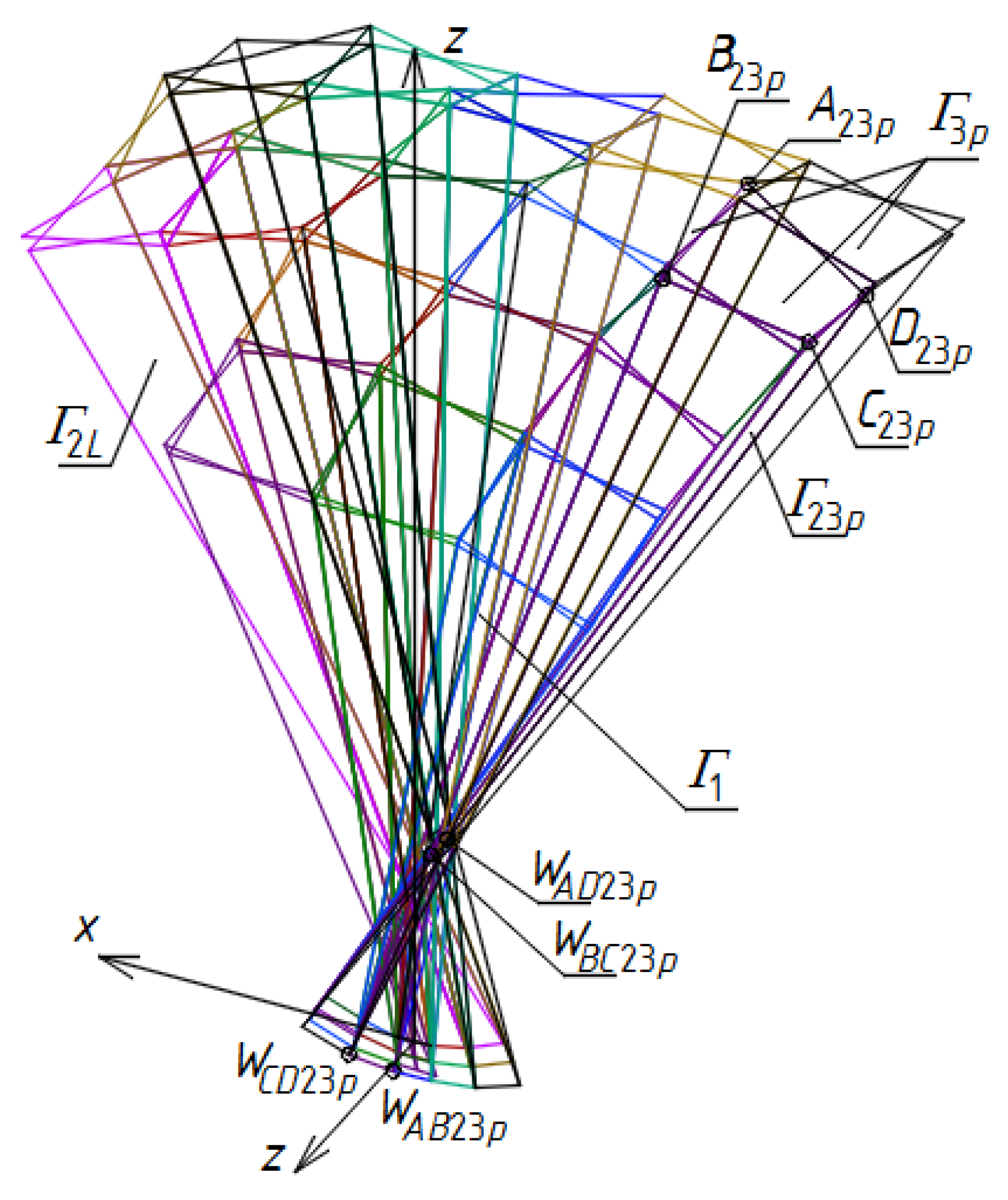
To create the third pair of the subnets Γ_3p and B_v3p of Γ and B_v, a (x,z)-plane-symmetry, of the previously constructed nets Γ₁ and B_v1 is used. Based on this symmetry, the following are transformed: (1) all vertices W_ABij, W_CDij, W_ADij, and W_BCij of Γ₁, (2) all vertices A_ij, B_ij, C_ij, and D_ij of B_v1, (3) the points S_Aij, S_Bij, S_Cij, and S_Dij of ω_r. As a result of this transformation, the vertices W_ABijp, W_CDijp, W_ADijp, and W_BCijp of Γ_3p, the vertices A_ijp, B_ijp, C_ijp, and D_ijp of B_vijp and the points S_Aijp, S_Bijp, S_Cijp, and S_Dijp of ω_r are determined, Figure 34. The obtained points S_Aijp, S_Bijp, S_Cijp, S_Dijp, A_ijp, B_ijp, C_ijp, and D_ijp belong to the subspace contained between the planes (x,z) and (y,z), so that both the negative x-half-axis and the negative y-half-axis are included in this subspace. Examples of the reference tetrahedron Γ_23p of Γ_3p and the mesh B_v23p of B_v3p are shown in Figure 34.

For the subnets Γ_3p and B_v3p, many specific proportions between their side edge and axis lengths and angle measures similar to those obtained for Γ₁ and B_v1 can be found. Some relations resulting from the (x,z)-plane-symmetry of the vertices of Γ_3p and B_v3p and the corresponding vertices of Γ₁ and B_v1 created previously are listed in

Table A7. The coordinates of the vertices W_ABijp, W_CDijp, W_ADijp, W_BCijp (for i, j = 1, 2, 3) of the polyhedral reference network Γ_3p shown in Figure 29.

Vertex	x-Coordinate [mm]	y-Coordinate [mm]	z-Coordinate [mm]
WAB22p	xWAB22	−yWAB22	zWAB22
WCD22p	xWCD22	−yWCD22	zWCD22
WAD22p	xWBC22	−yWBC22	zWBC22
WBC22p	xWAD22	−yWAD22	zWAD22
WAB23p	xWAB23	−yWAB23	zWAB23
WCD23p	xWCD23	−yWCD23	zWCD23
WAD23p	xWBC23	−yWBC23	zWBC23
WBC23p	xWAD23	−yWAD23	zWAD23
WAB32p	xWAB32	−yWAB32	zWAB32
WCD32p	xWCD32	−yWCD32	zWCD32
WAD32p	xWBC32	−yWBC32	zWBC32
WBC32p	xWAD32	−yWAD32	zWAD32
WAB33p	xWAB33	−yWAB33	zWAB33
WCD33p	xWCD33	−yWCD33	zWCD33
WAD33p	xWBC33	−yWBC33	zWBC33
WBC33p	xWAD33	−yWAD33	zWAD33

,

Table A8. The coordinates of the points S_Aijp, S_Bijp, S_Cijp, S_Dijp for (i, j = 1, 2, 3) of the reference surface ω_r.

Point	x-Coordinate [mm]	y-Coordinate [mm]	z-Coordinate [mm]
SA22p	xSB22	−ySB22	zSB22
SB22p	xSA22	−ySA22	zSA22
SC22p	xSD22	−ySD22	zSD22
SD22p	xSC22	−ySC22	zSC22
SA23p	xSB23	−ySB23	zSB23
SB23p	xSA23	−ySA23	zSA23
SC23p	xSD23	−ySD23	zSD23
SD23p	xSC23	−ySC23	zSC23
SA32p	xSB32	−ySB32	zSB32
SB32p	xSA32	−ySA32	zSA32
SC32p	xSD32	−ySD32	zSD32
SD32p	xSC32	−ySC32	zSC32
SA33p	xSB33	−ySB33	zSB33
SB33p	xSA33	−ySA33	zSA33
SC33p	xSD33	−ySD33	zSD33
SD33p	xSC33	−ySC33	zSC33

and

Table A9. The coordinates of the vertices A_ijp, B_ijp, C_ijp, D_ijp, (for i, j = 1, 2, 3) of the eaves edge net B_v3p.

Point	x-Coordinate [mm]	y-Coordinate [mm]	z-Coordinate [mm]
A22p	xA32	−yA32	zA32
B22p	xB12	−yB12	zB12
C22p	xC12	−yC12	zC12
D22p	xD32	−yD32	zD32
A23p	xA33	−yA33	zA33
B23p	xB13	−yB13	zB13
C23p	xC13	−yC13	zC13
D23p	xD33	−yD33	zD33
A32p	xC31	−yC31	zC31
B32p	xB22	−yB22	zB22
C32p	xC22	−yC22	zC22
D32p	xB33	−yB33	zB33
A33p	xC32	−yC32	zC32
B33p	xB23	−yB23	zB23
C33p	xC23	−yC23	zC23
D33p	−22,940.0	23,014.0	48,143.90

posted in Appendix A. Table A7 relates to the vertices W_ABijp, W_CDijp, W_ADijp, and W_BCijp of Γ_3p. Table A8 concerns the points S_Aijp, S_Bijp, S_Cijp, and S_Dijp of ω_r. Table A9 applies to the vertices A_ijp, B_ijp, C_ijp, and D_ijp of B_v3p.

To determine the fourth subset Γ_4r of Γ and subnet B_v4r of B_v, a (y,z)-plane-symmetry of Γ₁ and B_v1 is used. The positions of the vertices W_ABijr, W_CDijr, W_ADijr, and W_BCijr of Γ_4r, the vertices A_ijr, B_ijr, C_ijr, and D_ijr of B_vijr and the points S_Aij, S_Bij, S_Cij, and S_Dij of ω_r are determined as a result of the transformations of (1) the vertices W_ABij, W_CDij, W_ADij, and W_BCij of Γ₁, (2) the vertices A_ij, B_ij, C_ij, and D_ij of B_v1, (3) the points S_Aij, S_Bij, S_Cij, and S_Dij of ω_r, so that S_Aijr, S_Bijr, S_Cijr, S_Dijr, A_ijr, B_ijr, C_ijr, and D_ijr belong to the dihedral angle limited by the (x,z)-half-plane and (y,z)-half-plane containing the positive x-half-axis and the positive y-half-axis, Figure 26.

Some selected relations between the vertices of Γ_4r and B_v4r and the corresponding vertices of Γ₁ and B_v1, resulting from the (y,z)-plane-symmetry of Γ and B_v are given in

Table A10. The coordinates of the vertices W_ABijr, W_CDijr, W_ADijr, W_BCijr (for i, j = 1, 2, 3) of the polyhedral reference network Γ_4r shown in Figure 21.

Vertex	x-Coordinate [mm]	y-Coordinate [mm]	z-Coordinate [mm]
WAB22r	−xWCD22	yWCD22	zWCD22
WCD22r	−xWAB22	yWAB22	zWAB22
WAD22r	−xWAD22	yWAD22	zWAD22
WBC22r	−xWBC22	yWBC22	zWBC22
WAB23r	−xWCD23	yWCD23	zWCD23
WCD23r	−xWAB23	yWAB23	zWAB23
WAD23r	−xWAD23	yWAD23	zWAD23
WBC23r	−xWBC23	yWBC23	zWBC23
WAB32r	−xWCD32	yWCD32	zWCD32
WCD32r	−xWAB32	yWAB32	zWAB32
WAD32r	−xWAD32	yWAD32	zWAD32
WBC32r	−xWBC32	yWBC32	zWBC32
WAB33r	−xWCD33	yWCD33	zWCD33
WCD33r	−xWAB33	yWAB33	zWAB33
WAD33r	−xWAD33	yWAD33	zWAD33
WBC33r	−xWBC33	yWBC33	zWBC33

,

Table A11. The coordinates of the points S_Aijr, S_Bijr, S_Cijr, S_Dijr for (i, j = 1, 2, 3) of the reference surface ω_r.

Point	x-Coordinate [mm]	y-Coordinate [mm]	z-Coordinate [mm]
SA22r	−xSD22	ySD22	zSD22
SB22r	−xSC22	ySC22	zSC22
SC22r	−xSB22	ySB22	zSB22
SD22r	−xSA22	ySA22	zSA22
SA23r	−xSD23	ySD23	zSD23
SB23r	−xSC23	ySC23	zSC23
SC23r	−xSB23	ySB23	zSB23
SD23r	−xSA23	ySA23	zSA23
SA32r	−xSD32	ySD32	zSD32
SB32r	−xSC32	ySC32	zSC32
SC32r	−xSB32	ySB32	zSB32
SD32r	−xSA32	ySA32	zSA32
SA33r	−xSD33	ySD33	zSD33
SB33r	−xSC33	ySC33	zSC33
SC33r	−xSB33	ySB33	zSB33
SD33r	−xSA33	ySA33	zSA33

and

Table A12. The coordinates of the vertices A_ijr, B_ijr, C_ijr, D_ijr (for i, j = 1, 2, 3) of the eaves edge net B_v4r.

Point	x-Coordinate [mm]	y-Coordinate [mm]	z-Coordinate [mm]
A22r	−xA23	yA23	zA23
B22r	−xB23	yB23	zB23
C22r	−xC21	yC21	zC21
D22r	−xD21	yD21	zD21
A23r	−xC13	yC13	zC13
B23r	−xD33	yD33	zD33
C23r	−xC22	yC22	zC22
D23r	−xD22	yD22	zD22
A32r	−xA33	yA33	zA33
B32r	−xB33	yB33	zB33
C32r	−xC31	yC31	zC31
D32r	−xD31	yD31	zD31
A33r	−xC23	yC23	zC23
B33r	−xD33p	−yD33p	zD33p
C33r	−xC32	yC32	zC32
D33r	−xD32	yD32	zD32

included in Appendix A. Table A10 relates to the W_ABijr, W_CDijr, W_ADijr, and W_BCijr vertices of Γ_4r. Table A11 concerns the points S_Aijr, S_Bijr, S_Cijr, and S_Dijr of ω_r. Table A12 applies to the vertices A_ijr, B_ijr, C_ijr, and D_ijr of B_v4r. Finally, the sought-after nets Γ and B_v are created as the sums of the respective symmetric subnets Γ₁, B_v1, Γ_2L, B_v2L, Γ_3p, B_v3p, Γ_4r, and B_v4r have already been constructed. These nets have to be supplemented with roof shell sectors and a plain base to obtain complete building free form model.

7. Discussion

The proposed method for creating parametric spatial networks enables implementation of the novel algorithms in computer programs to conveniently and intuitively search for unconventional shapes and position of elevation walls and roof shells. The benefits of the parameterization include (1) the possibility of defining and reducing a number of the independent variables entered into the method’s algorithm, (2) specifying the special relations between dependent and independent variables to obtain the intuitiveness of the free form shaping, the regularity and respective curvature of the resultant complex shell roofs, (3) interesting outside roof and elevation patterns in an arrangement of many complete shell roof sectors and plane walls facets. The shape and mutual position parameterization of all reference tetrahedrons constituting the meshes of the investigated reference networks allowed developing various types of the innovative polyhedral reference networks. The activity aims at making a parametric description of these networks by means of the smallest possible number of independent variables so that such networks become regular and consistent, as well as determine diversified geometrical properties of the employed reference surfaces, including the negative, positive or zero Gaussian curvature, Figure 35 and Figure 36.

The points S_Aijk, S_Bijk, S_Cijk, and S_Dijk (for i, j = 1–3, k = ϕ, L, p, r, where ϕ is the empty set) used in the example presented in the previous section designate a regular double-curved surface ω_r characterized by the positive Gaussian curvature, Figure 26 and Figure 35, because the values of the proportions d_SAijk, d_SBijk, d_SCijk, and d_SDijk are bigger than 1.0. Double-curved surfaces having the negative Gaussian curvature can be obtained when the coefficients range from 0.0 to 1.0, Figure 36. The investigated method allows one to enter certain points to determine such networks Γ and B_v for which the resultant reference surface is a single-curved surface having the zero Gaussian curvature. For this case, selected groups of the axes of some reference tetrahedrons Γ_ij have to be contained in the same straight lines. This problem is going to be presented in further publications.

In the presented example, it was shown how to create a regular, spatial, polyhedral reference network Γ on the basis of which eaves quadrilateral network B_v determining an unconventional shell roof structure can be built. All Γ_ijk (for i, j = 1–3, k = ϕ, L, p, r) of Γ are tetrahedrons whose vertices, side edges, planes and axes take specific mutual positions influencing diversified types of the created reference surfaces ω_r and eaves roof networks B_v. Meshes Γ_ijk affect the rationality of the designed building free form structures due to the specific mutual positions of the side edges a_ijk, b_ijk, c_ijk and d_ijk of Γ. B_vijk (for i, j = 1–3, k = ϕ, L, p, r) of B_v are closed spatial quadrangles whose two opposite sides can be taken as roof directrices. The parametric shapes and mutual positions of the directrices may positively affect a process of designing the attractive building structures by automatically changing the proportions d_Aij, d_Bij, d_Cij, and d_Dij defining the positions of the B_vijk‘s vertices on a_ijk, b_ijk, c_ijk and d_ijk in accordance with ω_r.

The investigated method relies on special setting all subsequent reference tetrahedrons together, so that each pair of two adjacent tetrahedrons has one plane in common. Many reference tetrahedrons can be set together to obtain an edge roof shell structures having regular edge patterns on its surfaces and attractive patterns of folded plane areas on its elevations. The analyzed specific properties of the innovative spatial reference networks should lead to a creative intuitive computational shaping of attractive, rational complex-building free forms of medium and large span and novel structural systems intended for these forms.

The network B_v introduced in Section 6, Figure 26, and the network shown in Figure 36 are characterized by the fact that each pair of their adjacent quadrilateral meshes B_vijk and B_vmns arranged orthogonally in relation to the mesh B_v11 (for i = 1 or j = 1 and m = 1 or n = 1 and k, s = ϕ, L, p, r) has one common edge, including their directrix, and two common vertices. In addition, each tetrad of adjacent quadrilaterals B_vijk has one common vertex. In contrast, the B_v network shown in Figure 35 was created so that each of the two adjacent quadrangles B_vijk and B_vmns arranged in any of the orthogonal directions compatible with the principal planes (x,z) and (y,z) do not have a common edge, but their corresponding edges are inclined to each other and intersect in one point. In this case, each two adjacent meshes-quadrangles arranged diagonally in B_v have only one common vertex.

The shell roof structure Ω presented in Section 6 is continuous and has many edges between smooth sectors Ω_ijk limited by eaves quadrangles B_vijk (for i = 1 or j = 1 and m = 1 or n = 1 and k = ϕ, L, p, r). The edges model a set of ribs between the complete transformed shells of a roof structure. In the parametric description of Γ implemented to computer applications, it is possible to easily change the positions of all vertices A_ijk, B_ijk, C_ijk, D_ijk of the meshes B_vijk along the side edges of Γ, relative to reference surface ω_r by modifying the division coefficients of some specific pairs of—the vertices of Γ. The change may cause the resultant structure Ω to become discontinuous, Figure 35. The structure Ω can contain many empty flat areas dividing the roof shell sectors Ω_ijk. These openings should be built by windows illuminating the interior of the designed building with the sunlight. This problem is also going to be analyzed in the further publications.

The author has developed some activities leading to minimize the number of independent parameters describing the geometrical properties of the presented reference networks. For this purpose, symmetrical forms of buildings must be sought. The possibility of adopting one parameter constituting only one independent variable used in defining all proportions between the selected roof and elevation elements is also developed by the author to find similar and different types of various free forms.

8. Conclusions

There are significant limitations in creating building free forms roofed with transformed corrugated shell sheeting concerning the complicated orthotropic geometrical and mechanical properties of thin-walled folded steel sheets. To overcome these limitations, the novel method based on the polyhedral reference networks and quadrilateral eaves nets helpful in shaping individual free forms and their specific multi-plane and multi-shell structures were carried out. As a result, the intuitive method supported by novel computer applications uses the presented relatively great possibilities of searching for diverse and innovative building structures based on the proposed shape transformations.

The main goals of combining the complete transformed shells in any roof structure include increasing the span of the roof and entire building, integrating the roof and façade forms, increasing the visual attractiveness of the entire building free form, and making it sensitive to the natural or built environments. The most common concept used in a shaping of such transformed folded shell structures is a combination of central sections of right hyperbolic paraboloids, their halves or quadrants set in various configurations, and joined along their common edges. The author developed many coherent rules for creating such complex structures covered with plane-walled folded elevations and multi-segment transformed shell roof structures. The developed algorithms allowed a radical increase in the variety of the shapes employed in design.

The presented method uses the novel vector and parametric descriptions of shaping complex building free forms characterized by the shape integration of their complex multi-shell roofs and multi-plane façades. The method’s algorithm requires entering specific sets of parameters defining the general shapes of the investigated complex free forms and their individual roof and elevation elements. The parameters are either the measures of the vectors and angles of stiff motions such as translations and rotations, or the division coefficients of certain characteristic points, of the proposed novel networks by their other characteristic points.

Many proportions between geometric properties of all roof and elevations elements can be defined using functions based on the measures of the investigated types of stiff motions to achieve diversified attractive patterns on multi-plane folded elevations and multi-shell roof structures. More comprehensive studies seem to be targeted at an assignment of (a) the possible types of the independent and dependent variables, (b) the specific proportions between the dependent parameters to obtain such specific groups of the architectural free forms that are characterized by similar or different properties, (c) the search for some ranges of the values of the selected independent parameters defining attractive building free forms.

Achieving optimal, rational and attractive solutions appearing as the result of the process of shaping building free forms roofed with transformed corrugated shells and their complete elements require using regularity and symmetry of (a) single reference tetrahedrons and entire reference polyhedral networks, (b) plane walls and entire elevations of the designed complex building free forms, (c) some strips of the transformed folded sheets and entire complete transformed roofs shells and their structures, (d) structural systems intended for these forms. The research initiated and developed by the author on parametric process of architectural, geometrical, and static strength shaping of the regular free form structures roofed with transformed corrugated shell structures, and their structural systems is very extensive and requires a certain number of complete steps. One of these steps associated with geometrical and computational shaping such forms was elaborated by the author and the obtained results are presented in this paper.

References

- Yu, W.-W.; LaBoube, R.A.; Chen, H. Cold Formed Steel Design; John Wiley and Sons Inc.: New York, NY, USA, 2000. [Google Scholar]
- Abdel_Sayed, G. Critical shear loading of curved panels of corrugated sheets. Proc. ASCE J. Struct. Div. 1970, 96, 1279–1294. [Google Scholar]
- Abramczyk, J. Shell Free Forms of Buildings Roofed with Transformed Corrugated Sheeting, Monograph; Publishing House of Rzeszow University of Technology: Rzeszów, Poland, 2017. [Google Scholar]
- Parker, J.E. Behavior of Light Gauge Steel Hyperbolic Paraboloid Shells. Ph.D. Thesis, Cornell University, Ithaca, NY, USA, 1969. [Google Scholar]
- Petcu, V.; Gioncu, D. Corrugated hypar structures. In Proceedings of the I International Conference on Lightweight Structures in Civil Engineering, Warsaw, Poland, 1 December 1995; pp. 637–644. [Google Scholar]
- Yang, H. A Finite Element Formulation for Stability Analysis of Doubly Curved Thin Shell Structures. Ph.D. Thesis, Cornell University, Ithaca, NY, USA, 1969. [Google Scholar]
- Prokopska, A.; Abramczyk, J. Parametric Creative Design of Building Free Forms Roofed with Transformed Shells Introducing Architect’s and Civil Engineer’s Responsible Artistic Concepts. Buildings 2019, 9, 58. [Google Scholar] [CrossRef] [Green Version]
- Abramczyk, J. Shape transformations of folded sheets providing shell free forms for roofing. In Proceedings of the 11th Conference on Shell Structures: Theory and Applications, Gdańsk, Poland, 11–13 October 2017; Pietraszkiewicz, W., Witowski, W., Taylor and Francis Group, Eds.; Routledge: London, UK, 2017; Volume 4, pp. 409–412. [Google Scholar]
- Prokopska, A.; Abramczyk, J. Shape Transformations of Plane Folded Sheets for Shell Roofing. IOP Conf. Ser. Mater. Sci. Eng. 2019, 471, 082064. [Google Scholar] [CrossRef]
- Reichhart, A. Geometrical and Structural Shaping Building Shells Made up of Transformed Flat Folded Sheets; Hhouse of Rzeszow University of Technology: Rzeszów, Poland, 2002. (In Polish) [Google Scholar]
- Abramczyk, J. Building Structures Roofed with Multi-Segment Corrugated Hyperbolic Paraboloid Steel Shells. Procedia Eng. 2016, 161, 1545–1550. [Google Scholar] [CrossRef] [Green Version]
- Nilson, V.E. Testing a light gauge steel hyperbolic paraboloid shell. Proc. ASCE J. Struct. Div. 1962, 88, 51–66. [Google Scholar]
- Winter, G. Strength of thin steel compression flanges. Trans. ASCE 1974, 112, 895–912. [Google Scholar]
- Muskat, R. Buckling of Light Gage Steel Hyperbolic Paraboloid Roofs. Ph.D. Thesis, Cornell University, Ithaca, NY, USA, 1968. [Google Scholar]
- Banavalkar, P.V. Analysis and Behavior of Light Gauge Hyperbolic Paraboloid Shells. Ph.D. Thesis, Cornell University, Ithaca, NY, USA, 1971. [Google Scholar]
- Gergely, P.; Banavalkar, P.V.; Parker, J.E. The Analysis and Behavior of Thin-Steel Hyperbolic Paraboloid Shells; A Research Project Sponsored by the America Iron and Steel Institute, Report No. 338; Civil, Architectural and Environmental Engineering: Ithaca, NY, USA, September 1971. [Google Scholar]
- McDermott, J.F. Single layer corrugated steel sheet hypars. Proc. ASCE J. Struct. Div. 1968, 94, 1279–1294. [Google Scholar]
- Gioncu, V.; Petcu, D. Corrugated Hypar Structures. In Proceedings of the International Conference LSCE, Warsaw, Poland, 25–29 September 1995; pp. 637–644. [Google Scholar]
- Egger, H.; Fischer, M.; Resinger, F. Hyperschale aus Profilblechen. Stahlbau 1971, 12, 353–361. [Google Scholar]
- Dawydov, J.U. House foods of Hyperbolic steel panel-shells. In Proceedings of the 12th International Conference on Supercomputing, ICS 1998, Melbourne, Australia, 13–17 July 1998; Volume II, pp. 500–550. [Google Scholar]
- Davis, J.M.; Bryan, E.R. Manual of Stressed Skin Diaphragm Design; Granada Publishing Ltd.: London, UK, 1982. [Google Scholar]
- Reichhart, A. Corrugated Deformed Steel Sheets as Material for Shells. In Proceedings of the International Conference on Lightweight Structures in Civil Engineering, Warsaw, Poland, 25–29 December 1995; pp. 625–636. [Google Scholar]
- Prokopska, A.; Abramczyk, J. Responsive Parametric Building Free Forms Determined by Their Elastically Transformed Steel Shell Roofs Sheeting. Buildings 2019, 9, 46. [Google Scholar] [CrossRef] [Green Version]
- Abramczyk, J. Transformed Shell Roof Structures as the Main Determinant in Creative Shaping Building Free Forms Sensitive to Man-Made and Natural Environments. Buildings 2019, 9, 74. [Google Scholar] [CrossRef] [Green Version]
- Abramczyk, J. Symmetric Shape Transformations of Folded Shell Roofs Determining Creative and Rational Shaping of Building Free Forms. Symmetry 2019, 11, 1438. [Google Scholar] [CrossRef] [Green Version]
- Biswas, M.; Iffland, J.S.B. Metal deks used to form hypar-shell panels. In Proceedings of the 2nd Speciality Conference on Cold-Formed Steel Structures, Rolla, MO, USA, 15–17 August 1973. [Google Scholar]
- Abramczyk, J. Parametric shaping of consistent architectural forms for buildings roofed with corrugated shell sheeting. J. Archit. Civ. Eng. Environ. 2017, 10, 5–18. [Google Scholar]
- Abramczyk, J. Principles of geometrical shaping effective shell structures forms. JCEEA 2014, XXXI, 5–21. [Google Scholar] [CrossRef]
- Prokopska, A.; Abramczyk, J. Innovative systems of corrugated shells rationalizing the design and erection processes for free building forms. J. Archit. Civ. Eng. Environ. 2017, 29–40. [Google Scholar] [CrossRef] [Green Version]
- Prokopska, A. Methodology of Architectural Design Preliminary Phases of the Architectural Process; Publishing House of Rzeszow University of Technology: Rzeszów, Poland, 2018. [Google Scholar]
- Abramczyk, J. Integrated building forms covered with effectively transformed folded sheets. J. Int. Assoc. Shell Spat. Struct. 2016, 57, 121–132. [Google Scholar] [CrossRef]
- Obrębski, J.B. Observations on Rational Designing of Space Structures. In Proceedings of the Symposium Montpellier Shell and Spatial Structures for Models to Realization IASS, Montpellier, France, 20–24 September 2004; pp. 24–25. [Google Scholar]
- Rębielak, J. Morphology of roof structure systems designer by means of lenticular girder. In Spatial Structures–Temporary and Permanent, Proceedings of the International Symposium of the International Association for Shell and Spatial Structures, Shanghai, China, 8–12 November 2010; Zhang, Q., Yang, L., Hu, Y., Eds.; China Architecture & Building Press: Shanghai, China, 2010; pp. 1249–1256. [Google Scholar]
- Abel, J.F.; Mungan, I. Fifty Years of Progress for Shell and Spatial Structures; International Association for Shell and Spatial Structures: Madrid, Spain, 2011. [Google Scholar]
- Dzwierzynska, J.; Prokopska, A. Pre-rationalized parametric designing of roof shells formed by repetitive modules of Catalan surfaces. Symmetry 2018, 10, 105. [Google Scholar] [CrossRef] [Green Version]
- Carmo, M.P. Differential Geometry of Curves and Surfaces; Prentice-Hall, Inc.: Englewood Cliffs, NJ, USA, 1976. [Google Scholar]
- Grey, A. Modern Differential Geometry of Curves and Surfaces with Mathematica; CRC Press LCC: Boca Raton, FL, USA, 1999. [Google Scholar]
- Żwirek, P. Selected issues of using nominally flat folded sheets and self-bearing panels for curved. In Proceedings of the 9th Scientific and Technical Conference on Shaping Structures. Thin-walled Structures, Rzeszów, Poland, 11–12 September 2015. (In Polish). [Google Scholar]
Figure 1.
Elastically bent corrugated cylindrical steel shells: (a) by Abdel_Sayed [2]; (b) by Abramczyk [3].
Figure 2.
Elastically twisted hyperbolic paraboloid steel shells: (a) two-layer by J.E. Parker [4]; (b) one-layer by Abramczyk [3].
Figure 3.
(a) An axis-symmetric experimental thin-walled corrugated steel shell supported by two curved skew directrices; (b) elements of a smooth model used for shaping the transformed shells.
Figure 4.
An accurate mechanical thin-walled folded model of a nominally plane folded sheet transformed elastically into a shell shape and the graphical expression of the “effective” stresses in MPa on its top surface.
Figure 5.
Two unconventional symmetric shell-free forms: (a) an erected roof shell by Reichhart [10]; (b) a computer model of a bar structural system intended for the transformed shell roof sheeting.
Figure 6.
A symmetric shell structure roofing the experimental hall at Rzeszow University of Technology: (a) an internal view; (b) an external view.
Figure 7.
Symmetrically arranged hyperbolic paraboloid units by Petcu and Gioncu [5]: (a) an erected corrugated umbrella shed; (b) various configurations of umbrella shell structures.
Figure 8.
Two symmetric experimental hyperbolic paraboloid shells: (a) a single shell by McDermott [17]; (b) an umbrella structure of four quarters by Banavalkar and Parker [16].
Figure 9.
The external view of one elevation of the experimental hall at Rzeszow University of Technology roofed with the shell structure.
Figure 10.
The first Field House structure proposed by Biswas and Iffland [26]: (a) concept and elevation; (b) plan.
Figure 11.
The second structure proposed by Biswas and Iffland [26]: (a) elevation; (b) framing plan of a quarter of the structure.
Figure 12.
Two complex building free forms covered with multi-segment roof shell structures and plane-walled folded glass elevations characterized by (a) curved roof directrices; (b) straight roof directrices.
Figure 13.
Creation of a coherent complex free form arranged over a double-curved reference ellipsoid: (a) a quarter of the final structure; (b) normals to the reference ellipsoid.
Figure 14.
The architectural study of a free form optimized on the basis of the investigated reference ellipsoid.
Figure 15.
Two steel structural systems supporting transformed folded sheets by Żwirek [38]: (a) the erection of the final shell roof; (b) experimental tests.
Figure 16.
Creation of a complex free form by means of a reference network Γ composed of tetrahedral meshes Γij (i = j = 1): (a) Γij before setting (b) Γij after setting in Γ.
Figure 17.
A complex free form building structure Σ roofed with a continuous shell structure: (a) edge model; (b) architectural stadium.
Figure 18.
Creation of Γ11: (a) vertices: WCD11, WAB11, WAD11 and WBC11; (b) side edges: a11 = (WAD11, WAB11), b11 = (WBC11, WAB11), c11 = (WCD11, WBC11) and d11 = (WAD11, WCD11).
Figure 19.
Two subsequent steps of the creation of Σ11: (a) vertices A11, B11, C11 and D11; (b) eaves Bv11.
Figure 20.
Two subsequent steps of the determination of (a) the vertices WAB12, WBC12, WAD12, WCD12 of Γ12; (b) the vertices A12, B12, C12, D12 of Bv12.
Figure 21.
Two subsequent steps of the method’s algorithm related to the construction of; (a) the vertices of Γ21; (b) the eaves side edges of Σ21.
Figure 22.
Two subsequent steps of the method’s algorithm related to the construction of (a) all vertices of Γ22; (b) all side edges of Σ22.
Figure 23.
Subsequent steps of the method’s algorithm concerning: (a) definition of the Γ’s axes; (b) creation of the vertices of Σ21, Σ22.
Figure 24.
Subsequent steps of the method’s algorithm related to the creation: (a) a quarter of Γ; (b) the entire network Γ and the reference surface ωr symmetrical about the z-axis.
Figure 25.
The final step of creating Σ and Ω symmetrical about the z-axis.
Figure 26.
A multi-segment reference network Γ composed of four symmetric subnets Γ1, Γ2L, Γ3p, and Γ4r.
Figure 27.
Creation of two initial reference tetrahedrons: (a) Γ11; (b) Γ12; and (c) a detail of Γ12.
Figure 28.
The step related to creation of Γ13: (a) vertices; (b) a general shape.
Figure 29.
The step related to creation of Γ21: (a) a general shape; (b) vertices.
Figure 30.
The step related to the creation of the reference tetrahedron Γ31: (a) a general shape; (b) vertices.
Figure 31.
Determination of Γ22: (a) a general shape; (b) vertices of Bv22; (c) vertices of Γ22.
Figure 32.
A quarter Γ1 of the entire reference network Γ.
Figure 33.
Two steps of the determination of the second quarter Γ2L of the designed z-axis-symmetric reference network Γ.
Figure 34.
Three quarters Γ1, Γ2L and Γ3p of the reference network Γ.
Figure 35.
A sum of many spatial quadrangular meshes arranged compatible with a regular surface of the positive Gaussian curvature by means of a polyhedral reference network determined on the basis of the pair of auxiliary orthogonal networks composed of plane meshes.
Figure 36.
A sum of many spatial quadrangular meshes arranged compatible with a regular surface of the negative Gaussian curvature by means of a polyhedral reference network determined on the basis of the pair of auxiliary orthogonal networks composed of plane meshes.