Article

Numerical Study of Suspension Filtration Model in Porous Medium with Modified Deposition Kinetics

by
Bekzodjon Fayziev
1,
Gafurjan Ibragimov
2,*,
Bakhtiyor Khuzhayorov
1 and
Idham Arif Alias
2
1
Department of Mathematical Modeling, Samarkand State University, Samarkand 140100, Uzbekistan
2
Department of Mathematics and Institute for Mathematical Research, Universiti Putra Malaysia, Serdang 43400, Selangor, Malaysia
*
Author to whom correspondence should be addressed.
Symmetry 2020, 12(5), 696; https://doi.org/10.3390/sym12050696
Submission received: 29 January 2020 / Revised: 17 February 2020 / Accepted: 20 February 2020 / Published: 1 May 2020

Abstract

:
Filtration is one of the most used technologies in chemical engineering. Development of computer technology and computational mathematics made it possible to explore such processes by mathematical modeling and computational methods. The article deals with the study of suspension filtration in a porous medium with modified deposition kinetics. It is suggested that deposition is formed in two types, reversible and irreversible. The model of suspension filtration in porous media consists of the mass balance equation and kinetic equations for each type of deposition. The model includes dynamic factors and multi-stage deposition kinetics. By using the symmetricity of porous media, the higher dimensional cases are reduced to the one-dimensional case. To solve the problem, a stable, effective and simple numerical algorithm is proposed based on the finite difference method. Sufficient conditions for stability of schemes are found. Based on numerical results, influences of dynamic factors on solid particle transport and deposition characteristics are analyzed. It is shown that the dynamic factors mainly affect the profiles of changes in the concentration of deposition of the active zone.

1. Introduction

The problem of filtering disperse systems in a porous medium is of big practical importance. Many technological processes, natural phenomena, production processes, etc. are associated with the flow of dispersed systems in porous [1,2] and fractured-porous media [3,4]. In contrast to the filtration of homogeneous liquids, when filtering disperse systems, a number of new phenomena arise, the study of which is very important for understanding the mechanisms of the filtration process. If we consider suspensions as dispersed, then the most important question is to study the processes of transport of the dispersed phase of solid particles in a porous medium, the interaction of these particles with the surface of the skeleton of a porous medium, deposition in the pore space, the release of pore channels from deposited particles, etc. Note that such questions were studied very poorly from both the theoretical and experimental sides. In industrial and natural conditions, there are only a few studies. Perhaps one of the reasons for the poor knowledge of the problem is the extreme complexity of the physical and mathematical modeling of particle transport processes in pore space [5]. Fast development of computer technology and computational mathematics in recent years allow us to use more complex models to describe the process.
It is obvious that the study of the filtration of disperse systems taking into account the deposition and release of particles in addition to the experimental direction should be based on mathematical models [6]. However, the specifics of filtering dispersed systems in comparison with filtering conventional homogeneous systems are not always possible to take into account in mathematical models. Moreover, the mechanism of the deposition of particles in pores and their release by the filtration flow has not yet been sufficiently studied, although experimental data convincingly show clogging of the pores and it is possible to fix the distribution of the impurity concentration along the length of the filtration zone [7,8]. The theoretical basis of filtration of inhomogeneous fluids can be found in the books of Ives [9] and Shekhtman [10].
From the above, we see that one of the most important tasks in the study of dispersed system filtration is the developing of mathematical models of the process that adequately reflect the basic characteristic properties of the process under study. Various approaches have been developed to simulate the suspended particle transport and deposition process in porous media or in literature, the so-called deep bed filtration, which can be arbitrarily divided into the so-called empirical models [11,12,13], network models [14,15,16], models for analyzing particle trajectories [17,18,19] and stochastic models [20,21,22].
In the empirical (phenomenological) approach, the mathematical model for suspension filtration in porous media consists of mass balance equation and capture kinetics [11,12,23,24,25,26,27,28,29,30]. Balance equation for three dimensional case is in the following form
( m c + ρ ) t + v c x + c y + c z = 0 ,
where c is the concentration of the suspension, v is the filtration velocity, m is the porosity of the medium, ρ is the concentration of deposition, t is the time, x ,   y ,   z are coordinates of space. This equation is symmetric with respect to x ,   y ,   z .
As mentioned in [31] the filters used in water purification have two main categories: symmetric (homogeneous) and asymmetric (anisotropic). The pores in symmetric filters have close to a uniform diameter throughout the depth of the filter. So, in homogeneous porous media all characteristics are the same in all directions of coordinates ( x ,   y ,   z ) . One can assume that particle concentration in the stream c and the velocity v is uniform across the filter cross-section. Accordingly, the expected depositions are uniform across the cross-section, too. These common assumptions mean that the model can be developed as one-dimensional in space. Balance equation in one-dimensional case takes the form [11,12,23,24,25,26,27,28,29,30]
( m c + ρ ) t + v c x = 0 ,
Kinetic equation is in following form [11,23,24,25,26,27,28]
ρ t = λ ( ρ ) c ,
where λ ( ρ ) is the coefficient characterizing the kinetics.
The first kinetic equation for deep bed filtration is given by Iwasaki [32]. Kinetic equations given in the literature can be divided into two approaches [6,12]: irreversible deposition, which means deposited particles never get back to flow again and reversible deposition, meaning some of the deposited particles may be detached from the media grain by the flow. Irreversible kinetic equations are usually given in the form (3), where λ ( ρ ) can be changed during the filtration. λ ( ρ ) can be increasing [32] or decreasing function [33], but in some cases a combination of both kinds of behaviour mentioned above [34] are used. First reversible kinetic equations given by Mints [35] mentioned and experimentally showed that during the filtration due to the increasing of pressure gradient, detachment of less strongly linked particles from grain occurs. This kind of process can be described in the form ρ / t = β a t t c β d e t ρ , where β a t t and β d e t phenomenological attachment and detachment coefficients respectively. In [12], given multistage deposition kinetics, in the first stage an irreversible layer is formed, then in the operable stage reversible deposition is formed.
In [12,28,29] mass balance equation is given with diffusion equation
( m c + ρ ) t + v c x = D 2 c x 2 ,
where D is diffusion (dispersion) coefficient.
In the last decade fractional diffusion equation is used for fractural porous media [3,4,36].
In the present paper, we consider the problem of filtering a suspension in a porous medium, taking into account the deposition of solid particles of the suspension in the pore volume and their release. For this we use the well-known model of Venitsianov [23,24] and suggest its modification. The problem is considered taking into account dynamic factors in the kinetics of deposition. To solve the problem, a numerical method is developed based on finite difference scheme. The stability of the method is proved. By using the symmetry properties of porous media, the model was reduced to a one-dimensional case. The numerical algorithm developed in the present paper can be easily used for 2D and 3D cases by using “alternating direction method”, which means the values of functions in new time layer will be found separately for each coordinate. Based on the numerical solution of the problem, the role of dynamic factors on the filtration and transport characteristics is estimated.

2. Formulation of the Problem

The deposition in the porous space of the deep bed filters has two forms—washable and nonwashable. Accordingly, the filter zones are called active and passive [23,24]. The active zones washed by the flow form a reversible deposition with a concentration of ρ a , passive zones that are stagnant form an irreversible deposition do the same with a concentration of ρ p . Denote the total filter capacity by ρ 0 . From the foregoing
ρ 0 = ρ a 0 + ρ p 0
where ρ a 0 and ρ p 0 are the capacities of the active and passive zones, respectively. The indicated capacities have dynamic characteristics. They depend not only on the “quality” of the dispersed phase but also on the speed and structure of the flow, as well as the geometry of the layer [23].
We consider a semi-infinite homogeneous media with an initial porosity m 0 , filled with a homogeneous liquid. At the point x = 0 , starting from t = 0 to when the reservoir enters the suspension with a concentration c 0 and filtration velocity v t = v 0 = const .
The system of equations for suspension filtration with two deposition zones with a constant speed regime consists of the equation of balance and kinetic equations for each zone, which in the one-dimensional case is represented as
m 0 c t + v c x + ρ a t + ρ p t = 0 ,
ρ a t = β a c ρ a ρ a 0 c 0 ,
ρ p t = β p ( ρ p ) c ,
where c is the concentration of the suspension (m 3 /m 3 ), v is the filtration velocity (m/s), m 0 is the initial porosity of the medium, ρ a is the concentration of deposition in the active zone (m 3 /m 3 ), ρ p is the concentration of deposition in the passive zone (m 3 /m 3 ), β a is the coefficient characterizing the kinetics in the active zone (1/s), β p is the coefficient (1/s) associated with the effect of compaction (aging) of the deposition, which was proposed as β p = α ρ p β p 0 [23],
α ( ρ p ) = 1 for ρ p ρ p 1 , ρ p 1 / ρ p for ρ p 1 < ρ p < ρ p 0   , 0 for ρ p = ρ p 0   ,
where ρ p 1 is the value of ρ p at which “aging” begins.
Therefore, at the beginning of deposition formation, α = 1 . Starting with a certain concentration of ρ p 1 , the value of α becomes less than 1, and a further decrease in α goes inversely with the amount of deposition ρ p . Finally, when the deposition concentration is close to saturation, α decreases more rapidly. This section is approximated by a step.
The system of Equations (6)–(8) is solved taking into account the above dependence (9) and with the following initial and boundary conditions
c ( x , 0 ) = 0 ,     ρ a ( x , 0 ) = ρ p ( x , 0 ) = 0 ,       c ( 0 , t ) = c 0 = const .

3. Finite Difference Schemes for Model

To solve problem (6)–(10), we apply the finite difference method [37,38,39,40,41]. In the area D = 0 x < ,    0 t T we introduce a net, where T is the maximum time during which the process is studied. For this, we divide the interval 0 ,   in steps h and 0 ,   T into J parts in steps of τ . As a result we have a net
ω h τ = x i ,   t j ,   x i = i h ,     i = 0 , 1 , ,      t j = j τ ,   j = 0 , 1 , , J ,       τ = T T J J .
Instead of functions c t ,   x , ρ a t ,   x , ρ p t ,   x we consider the net functions and denote their values at the nodes x i ,    t j by c i j , ρ a , i j , ρ p , i j , respectively.
Equation (6) is approximated on a grid ω h τ by the equation
m 0 c i j + 1 c i j τ + v c i j + 1 c i 1 j + 1 h + ρ a , i j + 1 ρ a , i j τ + ρ p , i j + 1 ρ p , i j τ = 0 .
The difference scheme for Equation (7) will have the form
ρ a , i j + 1 ρ a , i j τ = β a c i j ρ a , i j ρ a 0 c 0 .
The difference scheme for Equation (8) is
ρ p , i j + 1 ρ p , i j τ = α ρ p , i j β p 0 c i j .
The initial and boundary conditions (10) are also presented in a net form as follows
ρ a , i j = 0 , i = 0 , I ¯ , j = 0 , ρ p , i j = 0 , i = 0 , I ¯ , j = 0 , c i j = 0 , i = 0 , I ¯ , j = 0 , c i j = c 0 , i = 0 , j = 0 , J ¯ ,
where I is a sufficiently large number for which the equation c I j = 0 is approximately satisfied.

4. Stability of the Finite Difference Schemes

Theorem 1.
The sufficient stability conditions for the initial data of the schemes (12) and (13) are
τ min 2 ρ a 0 β a c 0 ;   2 m 0 h β a h v + h α ( ρ p , i j ) β 0 , v < h ( β a + α ( ρ p , i j ) β 0 ) .
and the scheme (14) is unconditionally stable.
Proof of Theorem 1.
Schemes (12)–(14) are two-layer schemes. When studying the stability of two-layer schemes, we will use their canonical form [37]
B y t + A y = φ ( t ) ,     t = t n = n τ ω τ ,       y ( 0 ) = y 0 .
where y = y n = y ( t n ) ,    y ^ = y n + 1 = y ( t n + 1 ) = y ( t n + τ ) ,   y t = y ^ y τ , y n is vector-solution defined on the layer t n ,
y n = y 0 n ,   y 1 n ,   ,   y I n .
Let H h be a finite-dimensional real space, ( , ) be the scalar product, x = ( x , x ) is the norm in H h .
It is necessary to find sufficient conditions for the stability of the scheme (17) and obtain a priori estimates for its solution, expressing the stability of the scheme from the initial data.
The solution to the problem (17) can be represented in the form y = y ¯ + y ˜ , where y ¯ is a solution to the homogeneous equation with the initial condition y ¯   ( 0 ) = y ( 0 ) = y 0 :
B y t + A y = 0 ,     t ω τ ,       y ( 0 ) = y 0 ,
and y ˜ is a solution of a nonhomogeneous equation with zero initial condition
B y t + A y = φ ( t ) ,     t = ω τ ,       y ( 0 ) = 0 .
Estimation of the solution of problem (19)
y ( t + τ ) ( 1 ) M 1 y ( 0 ) ( 1 )
means that the scheme (17) is stable according to the initial data, and the estimate of the solution to the problem (20)
y ( t + τ ) ( 1 ) M 2 max 0 t t φ ( t ) ( 2 )
expresses the stability of the scheme (17) on the right hand side.
It is known [37] that the uniform stability of the scheme (19) from the initial data implies the stability of the scheme (20) on the right-hand side. Therefore, it is enough to show the uniform stability of the scheme (19). For this, it is necessary to obtain an a priori estimate such as
y n + 1 δ y n ,
for all n and for all y n , where δ n M 1 , δ and M 1 are independent of the net steps and n.
To study stability, a method based on an estimate of the norm of the transition operator from layer to layer can be applied.
We write the difference scheme (19) in the form
y ^ = S y ,    S = E τ B 1 A ,
where S is transition operator.
If A = A * > 0 , we can obtain the stability condition in the energy norms · A . From the inequality
y ^ A = S y A S A y A ,
it can be seen that the scheme (23) is stable in H A , if the norm of the transition operator does not exceed unity:
S A 1 .
We will check the inequality (24) for transition operators for (12)–(14).
The scheme (12) can be represented as
m 0 c i j + 1 c i j τ + v c i j + 1 c i 1 j + 1 h + β a c i j ρ a , i j ρ a 0 c 0 + α ρ p , i j β p 0 c i j = 0 .
We transform this equation to obtain
m 0 h ( c i j + 1 c i j ) + v τ ( c i j + 1 c i 1 j + 1 ) + τ h β a c i j ρ a , i j ρ a 0 c 0 + τ h α ρ p , i j β p 0 c i j = 0 ,
( m 0 h + v τ ) c i j + 1 = v τ c i 1 j + 1 + m 0 h τ h β a τ h α ρ p , i j β p 0 c i j τ h β a ρ a , i j ρ a 0 c 0 ,
c i j + 1 = m 0 h τ h β a τ h α ρ p , i j β p 0 m 0 h + v τ c i j + f ,
where f = 1 m 0 h + v τ v τ c i 1 j + 1 τ h β a ρ a , i j ρ a 0 c 0 . Introducing the solution vector c j = c 0 j ,   c 1 j ,     ,   c I j , from (25) discarding f (since stability is checked against the initial data) we get
c j + 1 S c j ,
where
S = m 0 h τ h β a τ h α ρ p , i j β p 0 m 0 h + v τ 1 .
This inequality is split down into two inequalities. The first one is
m 0 h τ h β a τ h α ρ p , i j β p 0 m 0 h + v τ 1 ,
m 0 h τ h β a τ h α ρ p , i j β p 0 m 0 h + v τ ,
τ h β a τ h α ρ p , i j β p 0 v τ ,
h β a + α ρ p , i j β p 0 v .
The validity of this inequality is obvious, since the left hand side is negative and the right hand side is positive. So let us look at the second inequality
1 m 0 h τ h β a τ h α ρ p , i j β p 0 m 0 h + v τ ,
m 0 h v τ m 0 h τ h β a τ h α ρ p , i j β p 0 ,
τ h β a + h α ρ p , i j β p 0 v 2 m 0 h .
By the second inequality in (16) v < h ( β a + α ( ρ p , i j ) β 0 ) , and hence
τ 2 m 0 h β a h v + h α ( ρ p , i j ) β 0 ,
We transform (13) to obtain
ρ a , i j + 1 = ρ a , i j + τ β a c i j ρ a , i j ρ a 0 c 0 ,
whence
ρ a , i j + 1 = ρ a , i j 1 τ β a c 0 ρ a 0 + τ β a c i j .
Ignoring the term τ β a c i j and introducing the solution vector ρ a , j = ρ a , 0 j ,   ρ a , 1 j ,     ,   ρ a , I j the scheme is written as
ρ a , j + 1 = S · ρ a , j ,
where S = 1 τ β a c 0 ρ a 0 E , E is unit operator.
Condition S 1 gives 1 τ β a c 0 ρ a 0 1 , from which we can find τ 2 ρ a 0 β a c 0 .
From (14) we obtain
ρ p , i j + 1 = ρ p , i j + τ α ρ p , i j β p 0 c i j
If ρ p , i j ρ p 1 , then α ρ p , i j = 1 and hence ρ p , i j + 1 = ρ p , i j + τ β p 0 c i j . Ignoring the term τ β p 0 c i j and by introducing the solution vector ρ p , j = ρ p , 0 j ,   ρ p , 1 j ,     ,   ρ p , I j last formula can be written in the form
ρ p , j + 1 = S · ρ p , j ,
where S = E , S = 1 .
If ρ p 1 < ρ p , i j < ρ p 0 , then α ρ p , i j = ρ p 1 ρ p , i j ,
ρ p , i j + 1 = ρ p , i j + τ ρ p 1 ρ p , i j β p 0 c i j .
Since ρ p 1 < ρ p , i j < ρ p 0 , then 0 < ρ p 1 ρ p , i j < 1 , we will take the maximum value,
ρ p , i j + 1 = ρ p , i j + τ β p 0 c i j .
ρ p , j + 1 = S · ρ p , j ,    S = E ,     S = 1 .
If ρ p , i j = ρ p 0 , then α ρ p , i j = 0 and ρ p , i j + 1 = ρ p , i j , ρ p , j + 1 = S · ρ p , j ,
S = E ,     S = 1 .
Let us look to another difference scheme. Let us introduce implicit schemes for (7) and (8) in the form
ρ a , i j + 1 ρ a , i j τ = β a c i j + 1 ρ a , i j + 1 ρ a 0 c 0 ,
ρ p , i j + 1 ρ p , i j τ = α ρ p , i j + 1 β p 0 c i j
instead of explicit schemes (13) and (14).
Theorem 2.
Scheme (26) is unconditionally stable, but scheme (27) is unstable.
Proof Theorem 2.
Since
ρ a , i j + 1 1 + τ c 0 ρ a 0 = ρ a , i j + τ β a c i j + 1 ,
we obtain
ρ a , i j + 1 = 1 + τ c 0 ρ a 0 1 ρ a , i j + τ β a c i j + 1 .
Clearly,
1 + τ c 0 ρ a 0 1 < 1 .
Therefore scheme (26) is unconditionally stable.
Next, for (27), if
ρ p 1 < ρ p , i j + 1 < ρ p 0 , t h e n    α ρ p , i j + 1 = ρ p 1 ρ p , i j + 1 .
Using the Taylor series, we obtain
α ρ p , i j + 1 = ρ p 1 ρ p , i j + ρ p , i j + 1 ρ p , i j 1 ρ p 1 ρ p , i j 2 ,
and so
ρ p , i j + 1 = ρ p , i j + ρ p 1 ρ p , i j + ρ p , i j + 1 ρ p , i j 1 ρ p 1 ρ p , i j 2 τ β p 0 c i j .
Finally,
ρ p , i j + 1 = ρ p , i j 2 + 2 ρ p 1 τ β p 0 c i j ρ p , i j 2 + ρ p 1 τ β p 0 c i j · ρ p , i j .
It is obvious that
ρ p , i j 2 + 2 ρ p 1 τ β p 0 c i j ρ p , i j 2 + ρ p 1 τ β p 0 c i j > 1 .
meaning that scheme (27) is unstable. □
It is unexpected that, in some cases explicit difference schemes are “better” than implicit ones.

5. Numerical Algorithm

Transforming the difference schemes (12)–(14) we get
c i j + 1 = h v τ + h m 0 v τ h c i 1 j + 1 + m 0 c i j ρ a , i j + 1 ρ a , i j + ρ p , i j + 1 ρ p , i j ,
ρ a , i j + 1 = ρ a , i j + τ β a c i j ρ a , i j ρ a 0 c 0 ,
ρ p , i j + 1 = ρ p , i j + τ α ρ p , i j β p 0 c i j ,
where
α ( ρ p , i j ) = 1 for ρ p , i j ρ p 1 , ρ p 1 ρ p 1 ρ p , i j ρ p , i j for ρ p 1 < ρ p , i j < ρ p 0   , 0 for ρ p , i j = ρ p 0   .
The system (28)–(30) is solved under the known initial and boundary conditions (15). The calculations are carried out in the following order. According to (29) and (30), the values ρ a , i j + 1 and ρ p , i j + 1 are determined through the known quantities ρ a , i j , ρ p , i j and c i j of the lower layer at the corresponding points, from (28) we determine c i j + 1 .

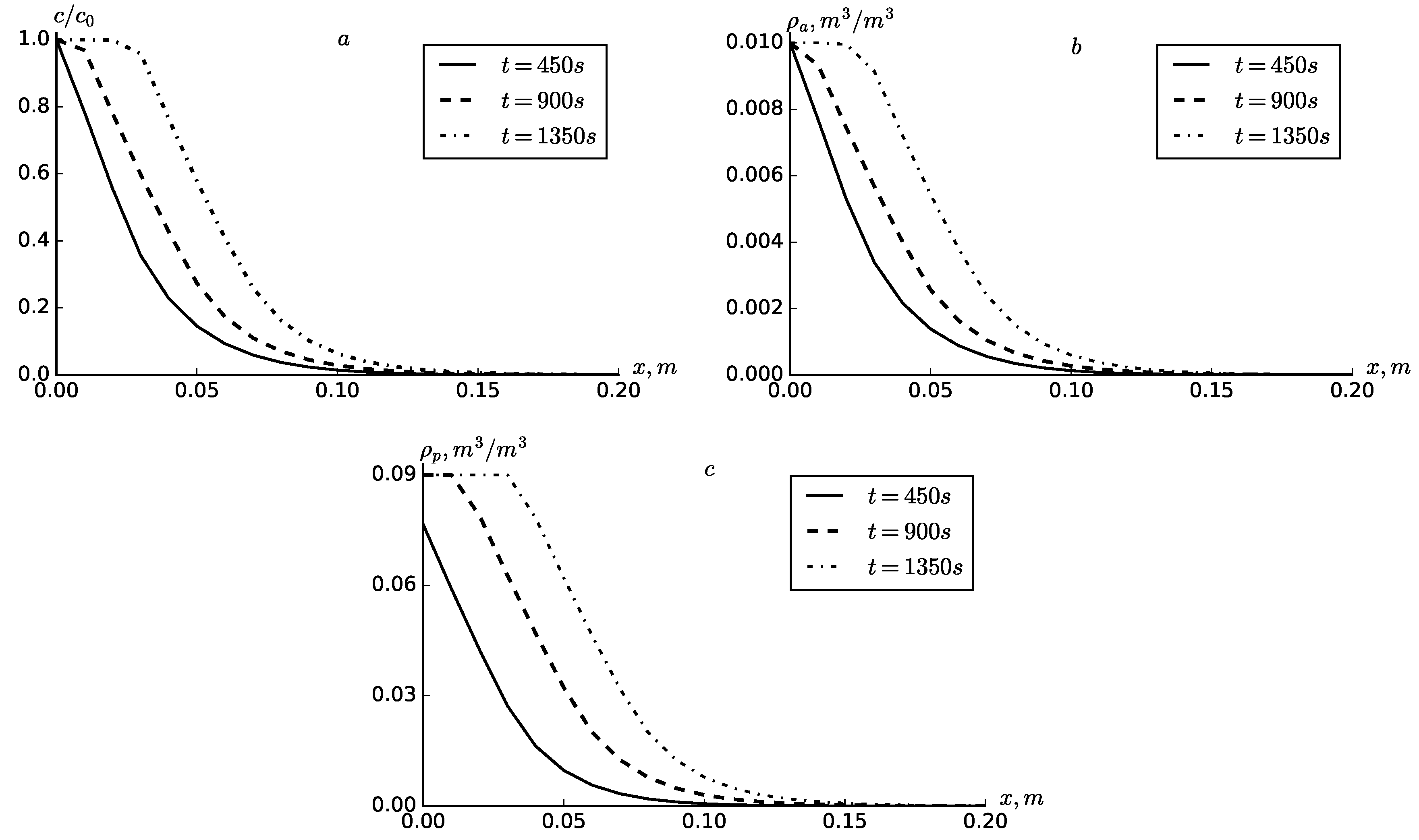
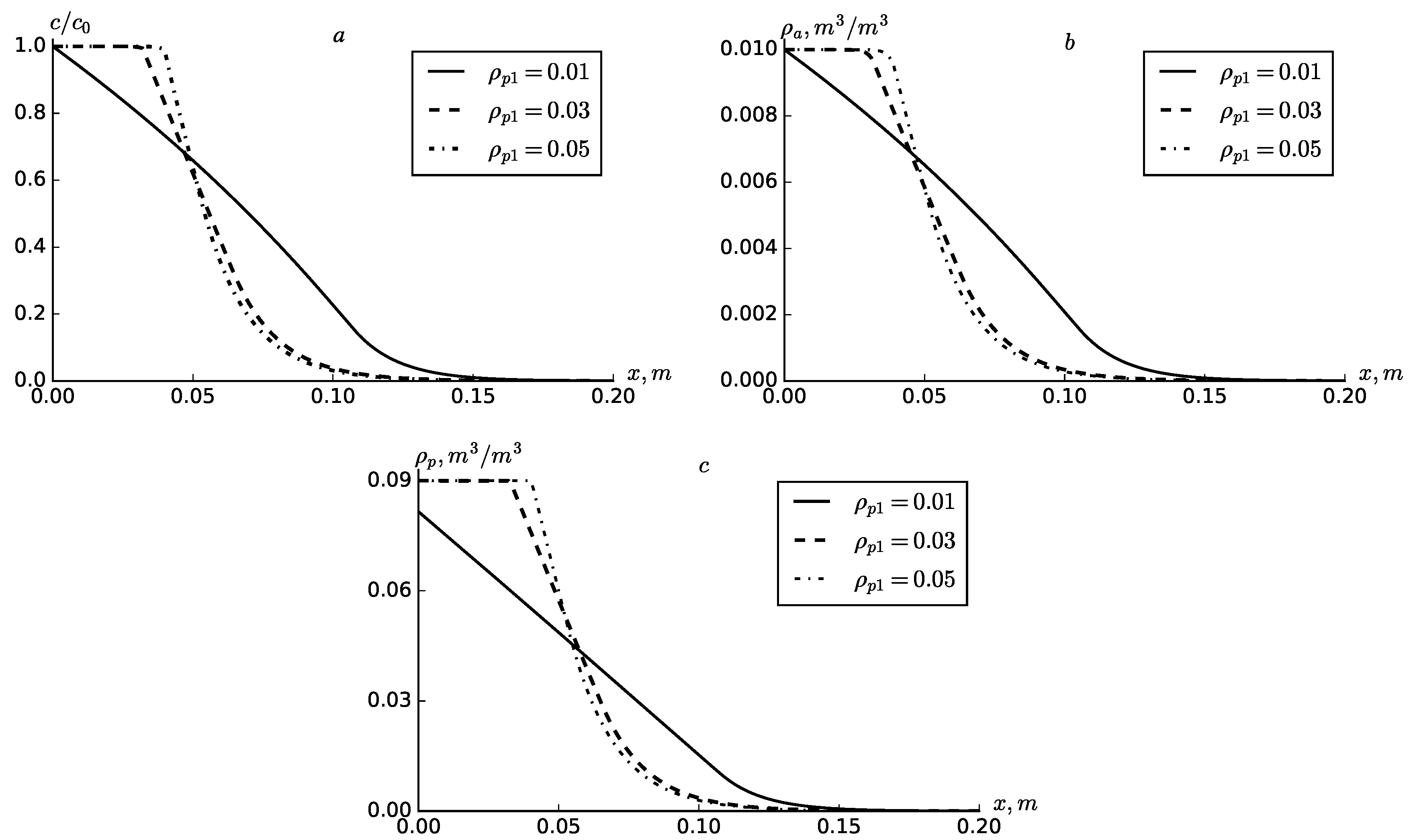
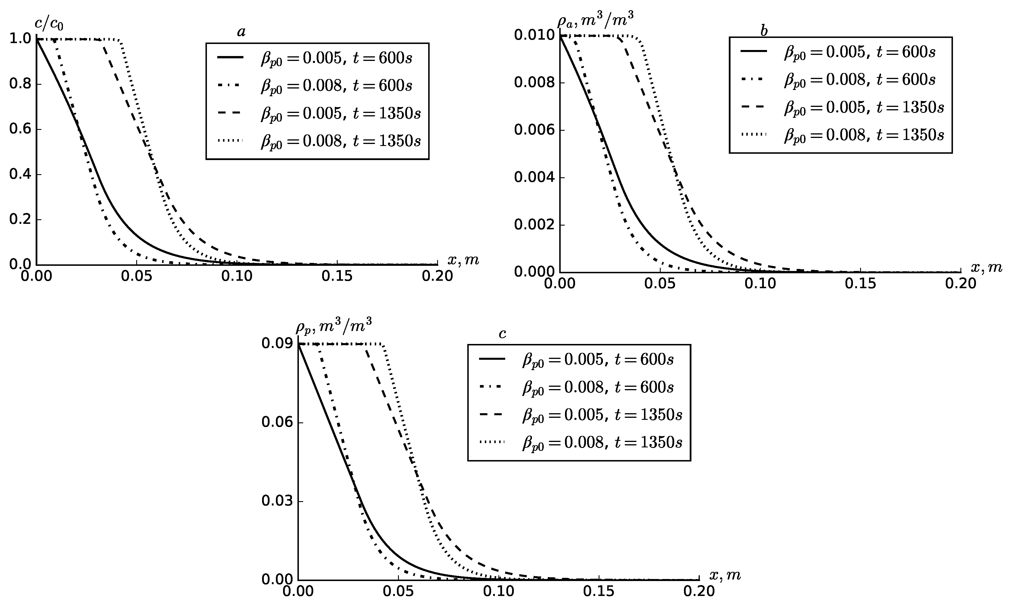
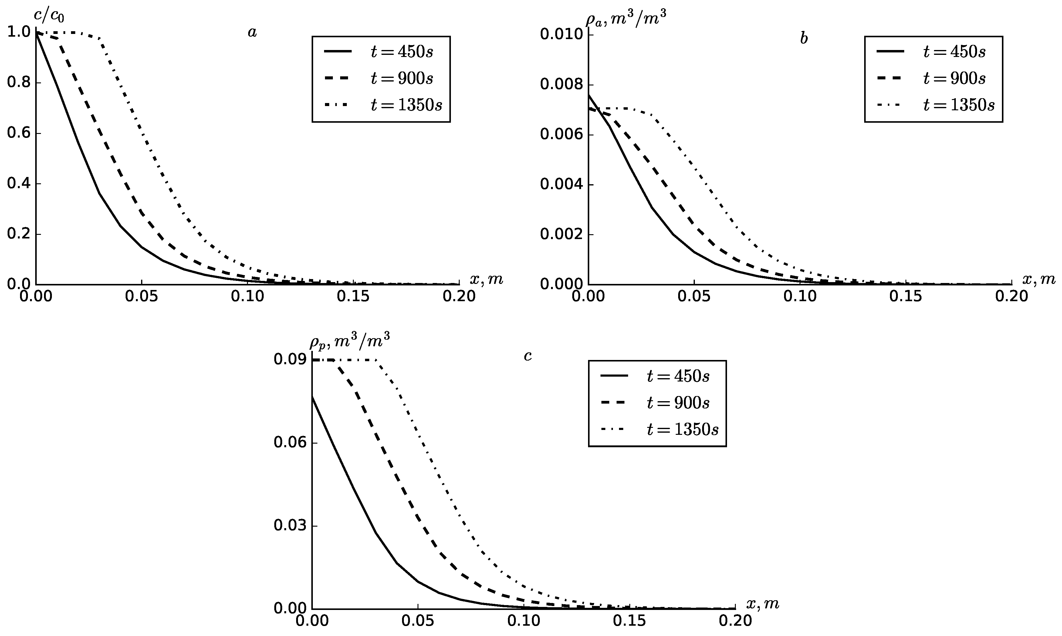
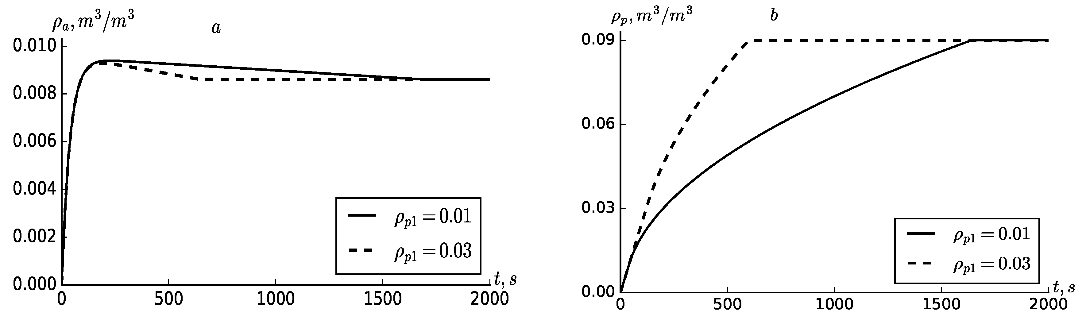
6. Numerical Experiments and Their Analyses

To carry out numerical experiments we developed a program in Python.
As the initial parameters, we take the following numerical values as [23,24]: c 0 = 0.05 , m 0 = 0.3 , v 0 = 10 4 m/s, ρ 0 = 0.1 , ρ a 0 = 0.01 , ρ p 0 = 0.09 , β a 0 = 0.005 s 1 , β p 0 = 0.005 s 1 .
Let us analyse the numerical results. Over time, the values of c, ρ a and ρ p at fixed points in the reservoir increase (Figure 1). With an increase in the parameter ρ p 1 to 0.05 at t = 450 s (Figure 1), near the point x = 0 , the capacitance of the passive zone is completely saturated with deposition and this leads to an increase in the concentration of suspended solids in the liquid c and deposition in the active zone ρ a . Increasing the parameter ρ p 1 leads to a delay in the front of the advance c, ρ a and ρ p .
Figure 2 shows graphs of the characteristics of the solute transport for various ρ p 1 , which allow us to estimate the effect of this parameter. As can be seen from the figures, nonmonotonic changes in all characteristics occur. An increase in ρ p 1 leads to a progressive dynamics of c c c 0 c 0 , ρ a , ρ p for small x and for relatively large x the opposite is observed.
It can be seen from Figure 3 that increasing the value of the parameter β p 0 leads to increased “ageing”, that is the concentration of irreversible deposition increases near the point x = 0 . This leads to an increase in the concentration of reversible deposition and concentrations of suspended particles. However, at the points away from x = 0 we can see the opposite scene. Most of the particles are deposited near the point x = 0 and this does not lead to distribution of suspended particles further. Figure 4 shows the time of the beginning of ageing according to the coordinate for various values of ρ p 1 . For ρ p 1 = 0.01, ageing is started at the point x = 0.02 approximately at t = 150 s, and for ρ p 1 = 0.03 at t = 350 s, for ρ p 1 = 0.05 at t = 550 s (Figure 4).

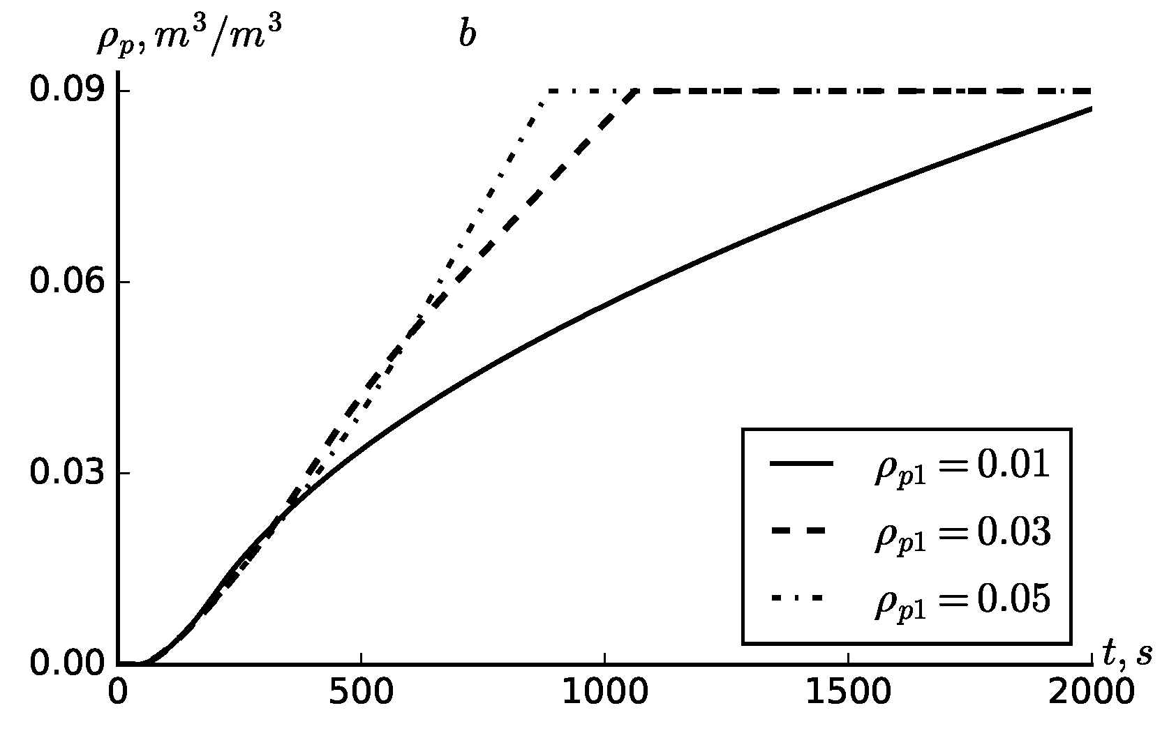
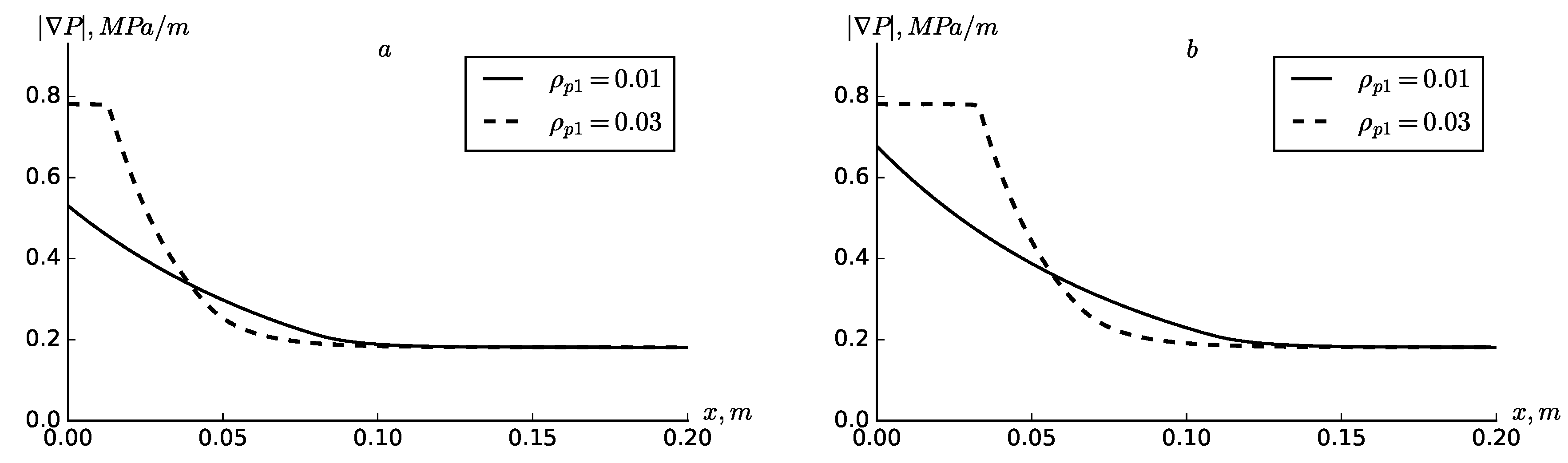
7. Improving the Model

Over the time when deposition is increasing it leads to change in porosity and permeability of porous media. Changes in porosity can be written as m = m 0 ρ a + ρ p . It also leads to change in filtration coefficient K m . Several formulas have been obtained for filtration coefficient in terms of porosity. Of these formulas the Carman–Kozeny formula [42,43,44] is widely used, which was developed for laminar flow in a packed bed of spherical grains. In our case porous media is homogenous and filtration velocity is small enough. So, for K m , we use Carman–Kozeny equation [42,43,44]
K m = k 0 m 3 k 0 m 3 1 m 1 m 2 ,
where k 0 = c o n s t is initial permeability coefficient of media before deposition occurs.
In constant flow regime, increasing of porosity and permeability leads to change in pressure gradient also. Darcy’s law basically used an equation describing the flow of a fluid through a porous medium. To find pressure gradient, we use Darcy’s law [26,27], which was first determined experimentally by Darcy, but it can be derived from the Navier–Stokes equations for small Reynolds numbers when inertial effects are ignored. In our case filtration velocity is small enough and we can ignore inertial effects, and so we use Darcy’s law in the form
v = K m p ,
where p is module of pressure gradient.
In [42], kinetic equations of the process of deposition (capture) of solid particles of a suspension as well as their release were generalised, taking into account dynamic factors. In accordance with [42], the process of particle deposition and release depends on the pressure gradient, and the greater module of pressure gradient the smaller probability of the deposition of the particles and greater the probability of the release of the particles from pores. In accordance with [42,45], the kinetic Equation (7) characterising the deposition and release of solid particles in the active zone of the porous medium is written as
ρ a t = β a 1 + γ p c β a ρ a 1 + ω p ρ a 0 c 0 .
where, constant parameters γ and ω characterise the intensity of the influence of p on attachment and detachment of particles, respectively.
Thus, model of suspension filtration in porous media taking into account changes in porous medium and dynamical factors consists of (6), (8), (31)–(33). The system of partial differential equations is solved under initial and boundary conditions (10) by using the finite difference schemes.
Some results are presented in Figure 5, Figure 6 and Figure 7. Dynamic factors mainly affect the profiles of changes in the concentration of the deposition in active zone. In the case when dynamic factors are not taken into account over time, the capacity of active zone ρ a 0 is completely saturated with deposition, here near the point x = 0 over time first ρ a increases, then decreases, and finally ρ a ρ a t t = 0 , even ρ a 0 is not completely saturated with deposition (Figure 5b). Why the capacity of active zone is not completely saturating with deposition can be explained by the fact that the capacity of active zone is dynamical. Which means by increasing the pressure gradient the structure of porous media can be partially destroyed and some previously deposited particles can get back to flow. This conclusion is quite consistent with conclusions of Mints [35]. The dynamical equilibrium, meaning that the number of deposited particles within the unit time is equal to the detached particles in this time in the active zone, occurs before the deposited particles volume get the capacity of the active zone. Dynamical equilibrium in active zone leads to an increase in suspended particles concentration which in turn leads to an increase in concentration of deposited particles in the passive zone. For ρ p 1 = 0.01 from t 1700   s and for ρ p 1 = 0.03 from t 600   s the dynamical equilibrium in active zone occurs, that is ρ a ρ a t t = 0 (Figure 6a). We can say that an increase in the parameters γ and ω leads to a decrease in ρ a at the corresponding points in the reservoir. Figure 7 shows the graphics of p for various ρ p 1 . For large values of ρ p 1 we can see the presence of large and almost constant values of p for small x, as in the previous cases, the nature of the p changes in greater values of x.

8. Discussion

On the basis of numerical analyses it has been established that for small values of ageing parameter, the deposition concentration in the passive zone still does not reach the capacitance of the passive zone in the studied times. With an increase in the ageing parameter near the point of inlet, the capacity of the passive zone is completely saturated with deposition and this leads to an increase in the concentration of suspended solids in fluid and the deposition in the active zone. It is shown that the consideration of dynamic factors mainly affects the profiles of changes in the concentration of the deposition in active zone. In the case when dynamic factors are not taken into account over time, the capacity of active zone is completely saturated with deposition. Here, near the inlet point over the time, deposition in active zone first increases, then decreases, and finally stops changing; even the capacity of active zone is not completely saturated with deposition. This can be explained as follows: over the time deposition is growing, it leads to a decrease of porosity and permeability. In constant, the filtration velocity regime decrease of porosity leads to an increase of pressure gradient. So, the probability of deposited particles detachment in the active zone increases and dynamical equilibrium (number of deposited and released particles in unity of time) occurs before the deposition reaches the capacity.

9. Conclusions

In this paper, the problem of filtration of a single-component suspension in a porous medium is posed. A mathematical model of suspension filtration in porous media is considered as a system of partial differential equations, which consists of mass balance equation, kinetic equations, Darcy’s law and Carman–Kozeny equation. The model takes into account the effects of ageing and dynamical factors. The influence of module of pressure gradient have been taken into account in kinetic equations directly. This allows us to estimate how the change in porous media characteristics affects particle deposition and release processes. To solve the problem, a numerical method has been developed on the basis of finite difference schemes. Though there are many finite difference schemes examined for partial differential equations, there are only a few examined for the system of partial differential equations. In addition, stability of difference schemes has been proved. As we know, implicit schemes are “better” than explicit schemes in stability, but in our case it has been shown that in some cases explicit schemes are more stable than implicit ones. To carry out numerical experiments, a program has been developed in Python.

Author Contributions

The authors contributed equally. All authors have read and agreed to the published version of the manuscript.

Funding

The present research was partially supported by Geran Putra Berimpak UPM/700-2/1/GPB/2017/ 9590200 of Universiti Putra Malaysia and by Ministry of Higher and Secondary Special Education of The Republic of Uzbekistan under the grant OT-F4-64 “Developing and numerical analysis of hydrodynamic models of filtration of liquid and solute transport in inhomogeneous porous media”.

Acknowledgments

The authors would like to thank the referees for the valuable comments that helped to improve the manuscript.

Conflicts of Interest

The authors declare no conflict of interest.

References

  1. Crittenden, J.C.; Harza, B.M. Water Treatment: Principles and Design, 3rd ed.; John Wiley and Sons Inc.: New York, NY, USA, 2012. [Google Scholar]
  2. Tarek, A.; McKinney, P.D. Advanced Reservoir Engineering; Gulf Professional Publishing: Burlington, VT, USA, 2005. [Google Scholar]
  3. Khuzhayorov, B.K.; Djiyanov, T.O.; Yuldashev, T.R. Anomalous Nonisothermal Transfer of a Substance in an Inhomogeneous Porous Medium. J. Eng. Phys. Thermophys. 2019, 92, 104–113. [Google Scholar] [CrossRef]
  4. Liu, R.; Jiang, Y. Fluid Flow in Fractured Porous Media; MDPI: Basel, Switzerland, 2019. [Google Scholar]
  5. Khuzhayorov, B.K. Filtration of Heterogeneous Liquids in Porous Media; Fan: Tashkent, Uzbekistan, 2005. (In Russian) [Google Scholar]
  6. Tien, C.; Ramarao, B.V. Granular Filtration of Aerosols and Hydrosols, 2nd ed.; Elsevier: Amsterdam, The Netherlands, 2007. [Google Scholar]
  7. Jegatheesan, V.; Vigneswaran, S. Deep Bed Filtration: Mathematical Models and Observations. Crit. Rev. Environ. Sci. Technol. 2005, 35, 515–569. [Google Scholar] [CrossRef]
  8. Zamani, A.; Maini, B. Flow of dispersed particles through porous media-deep bed filtration. J. Pet. Sci. Eng. 2009, 69, 71–88. [Google Scholar] [CrossRef]
  9. Ives, K.J. The Scientific Basis of Filtration. Nato Advanced Study Institutes Series. Series E: Applied Sciences; Noordhoff International Publishing: Leyden, The Netherlands, 1975. [Google Scholar]
  10. Shekhtman, Y.M. Filtration of Suspensions of Low Concentrations; Institute of Mechanics, USSR Academy of Science: Moscow, Russia, 1961. [Google Scholar]
  11. Herzig, J.P.; Leclerc, D.M.; Goff, P. Flow of suspensions through porous media—Application to deep filtration. Ind. Eng. Chem. 1970, 62, 8–35. [Google Scholar] [CrossRef]
  12. Gitis, V.; Rubinstein, I.; Livshits, M.; Ziskind, G. Deep-bed filtration model with multistage deposition kinetics. Chem. Eng. J. 2010, 163, 78–85. [Google Scholar] [CrossRef]
  13. Khuzhayorov, B.; Fayziev, B. A model of suspension filtration in porous media with multistage accumulation kinetics. Int. J. Adv. Res. Sci. Eng. Technol. 2017, 4, 4643–4648. [Google Scholar]
  14. Sharma, M.M.; Yortsos, Y.C. Transport of Particulate Suspensions in Porous Media. Model Formulation. AIChE J. 1987, 33, 1636–1643. [Google Scholar] [CrossRef]
  15. Rege, S.D.; Fogler, H.S. A Network Model for Deep Bed Filtration of Solid Particles and Emulsion Drops. AIChE J. 1988, 34, 1761–1772. [Google Scholar] [CrossRef]
  16. Yang, H.; Balhoff, M.T. Pore-network modeling of particle retention in porous media. AIChE J. 2017, 63, 3118–3131. [Google Scholar] [CrossRef]
  17. Payatakes, A.C.; Tien, C.; Turian, R.M. A new model for granular porous media. I. model formulation. AIChE J. 1973, 19, 58–76. [Google Scholar] [CrossRef]
  18. Rajagopalan, R.; Tien, C. Trajectory analysis of deep-bed filtration with sphere-in-cell porous media model. AIChE J. 1976, 22, 523–533. [Google Scholar] [CrossRef]
  19. Paraskeva, C.A.; Burganos, V.N.; Payatakes, A.C. A three-dimensional trajectory analysis of particle deposition in constricted tubes. Chem. Eng. Commun. 2007, 108, 23–48. [Google Scholar] [CrossRef]
  20. Litwiniszyn, J. Colmatage-Scouring Kinetics in the Light of Stochastic Birth-Death Process. Bull. Acad. Pol. Sci. Ser. Sci. Technol. 1966, 14, 81–85. [Google Scholar]
  21. Hsu, E.H.; Fan, L.T. Experimental Study of Deep Bed Filtration: A Stochastic Treatment. AIChE J. 1984, 30, 267–273. [Google Scholar] [CrossRef]
  22. Nassar, R.; Chou, S.T.; Fan, L.T. Modelling and simulation of deep-bed filtration: A stochastic compartmental model. Chem. Eng. Sci. 1986, 41, 2017–2027. [Google Scholar] [CrossRef]
  23. Venitsianov, E.V.; Rubinstein, R.N. Dynamics of Sorption from Liquid Media; Nauka: Moscow, Russia, 1983. (In Russian) [Google Scholar]
  24. Venitsianov, E.V.; Senyavin, M.M. Mathematical description of filtration clarification of suspensions. Theor. Found. Chem. Technol. 1976, 10, 584–591. (In Russian) [Google Scholar]
  25. Guedes, G.R.; Al-Abduwani, F.; Bedrikovetsky, P.; Currie, P. Deep-Bed Filtration under Multiple Particle-Capture Mechanisms. SPE J. 2009, 14, 477–487. [Google Scholar] [CrossRef] [Green Version]
  26. Malgaresi, G.; Khazali, N.; Bedrikovetsky, P. Non-monotonic retention profiles during axi-symmetric colloidal flows. J. Hydrol. 2020, 580, 124235. [Google Scholar] [CrossRef]
  27. Bedrikovetsky, P. Upscaling of stochastic micro model for suspension transport in porous media. Transp. Porous Med. 2008, 75, 335–369. [Google Scholar] [CrossRef]
  28. Bradford, S.A.; Simunek, J.; Bettahar, M.; van Genuchten, M.T.; Yates, S.R. Modeling colloid attachment, straining, and exclusion in saturated porous media. Environ. Sci. Technol. 2003, 37, 2242–2250. [Google Scholar] [CrossRef]
  29. Chrysikopoulos, C.V.; Katzourakis, V.E. Colloid particle size-dependent dispersivity. Water Resour. Res. 2015, 51, 4668–4683. [Google Scholar] [CrossRef]
  30. Boronin, S.A.; Tolmacheva, K.I.; Osiptsov, A.A.; Sitnikov, A.N.; Yakovlev, A.A.; Belozerov, B.V.; Belonogov, E.V.; Galeev, R.R. Damage to formation surrounding flooding wells: Modelling of suspension filtration with account of particle trapping and mobilization. J. Phys. Conf. Ser. 2017, 925, 012009. [Google Scholar] [CrossRef]
  31. Doran, P.M. Bioprocess Engineering Principles, 2nd ed.; Academic Press: Cambridge, MA, USA, 2013. [Google Scholar]
  32. Iwasaki, T. Some notes on sand filtration. J. Am. Water Works Assoc. 1937, 29, 1591–1602. [Google Scholar] [CrossRef]
  33. Mehter, A.A.; Turian, R.M.; Tien, C. Filtration in Deep Beds of Granular Activated Carbon; Research Report No. 70-3, FWPCA Grant No. 17020 OZO; Syracuse University: Syracuse, NY, USA, 1970. [Google Scholar]
  34. Ives, K.J. Rational design of filters. Proc. Inst. Civ. Eng. 1960, 16, 189–193. [Google Scholar] [CrossRef]
  35. Mints, D.M. Kinetics of filtration of low concentration water suspension in water purification filters. Dokl. Akad. Nauk 1951, 78, 315–318. (In Russian) [Google Scholar]
  36. Belevtsov, N.S.; Lukashchuk, S.Y. Symmetry group classification and conservation laws of the nonlinear fractional diffusion equation with the Riesz potential. Symmetry 2020, 12, 178. [Google Scholar] [CrossRef] [Green Version]
  37. Samarskii, A.A. The Theory of Difference Schemes; CRC Press: New York, NY, USA, 2001. [Google Scholar]
  38. Shampine, L.F. Two-step Lax-Friedrichs method. Appl. Math. Lett. 2005, 18, 1134–1136. [Google Scholar] [CrossRef] [Green Version]
  39. Golubev, V.I.; Mikhailov, D.N. Modeling the dynamics of filtration of a two-particle suspension through a porous medium. Works MIPT 2011, 3, 143–147. (In Russian) [Google Scholar]
  40. Thomas, J.W. Numerical Partial Differential Equations: Finite Difference Methods; Springer: New York, NY, USA, 1995. [Google Scholar]
  41. Strikwerda, J.C. Finite Difference Schemes and Partial Differential Equations, 2nd ed.; Society for Industrial and Applied Mathematics: Philadelphia, PA, USA, 2004. [Google Scholar]
  42. Khuzhaerov, B. Effects of blockage and erosion on the filtration of suspensions. J. Eng. Phys. 1990, 58, 185–190. [Google Scholar] [CrossRef]
  43. Zheng, X.L.; Shan, B.B.; Chen, L.; Sun, Y.W.; Zhang, S.H. Attachment–detachment dynamics of suspended particle in porous media: Experiment and modeling. J. Hydrol. 2014, 511, 199–204. [Google Scholar] [CrossRef]
  44. Hirabayashi, S.; Sato, T.; Mitsuhori, K.; Yamamoto, Y. Microscopic numerical simulations of suspension with particle accumulation in porous media. Powder Technol. 2012, 225, 143–148. [Google Scholar] [CrossRef]
  45. Khuzhaerov, B. Model of colmatage-suffosion filtration of disperse systems in a porous medium. J. Eng. Phys. 2000, 58, 668–673. [Google Scholar] [CrossRef]
Figure 1. Profiles of c / c 0 (a), ρ a (b), ρ p (c), at ρ p 1 = 0.03 .
Symmetry 12 00696 g001
Figure 2. Profiles of c / c 0 (a), ρ a ( b ) ,   ρ p (c), at t = 1350 s.
Symmetry 12 00696 g002
Figure 3. Profiles of c / c 0 (a), ρ a (b), ρ p (c), at different values of β p 0 .
Symmetry 12 00696 g003
Figure 4. Dynamics of ρ p at the point x = 0.02 m at different values of ρ p 1 .
Symmetry 12 00696 g004
Figure 5. Profiles of c / c 0 (a), ρ a (b), ρ p (c), at ρ p 1 = 0.03 ,   γ = 0.25 m/MPa, ω = 0.25 m/MPa, k 0 = 0.01 m 2 /(MPa · s).
Symmetry 12 00696 g005
Figure 6. Dynamics of ρ a (a) and ρ p (b) at the point x = 0 m at different values of ρ p 1 ,   γ = 0.1 m/MPa, ω = 0.1 m/MPa.
Symmetry 12 00696 g006
Figure 7. Profiles of p at t = 900   s (a), t = 1350   s (b) and at different values of ρ p 1 .
Symmetry 12 00696 g007

