Change Point Detection with Mean Shift Based on AUC from Symmetric Sliding Windows

Abstract

Change point detection is widely used in signal detection, industrial engineering, economy, finance, biomedicine and many other fields. The widely used parametric methods require prior knowledge of the noise signal distribution, which are seldom realistic. In practice, when the distribution of noise is not known, it is desirable to design algorithms based on non-parametric statistics, which, in the null case (no change point), are completely distribution free. To this end, we propose to use two symmetric sliding windows to compute the Area Under the receiver operating characteristic Curve (AUC) as a test statistic to measure the difference between the distribution of two samples. In the stage of change point detection, a threshold is designed according to hypothesis test which is based on the null distribution of the test statistics. This threshold is used to detect the potential change points in the signal. To reduce the probability of false alarm detection, a key parameter K is set to distinguish and delete the false alarms in potential change points. Comparative studies showed that our proposed method outperforms the classical Relative unconstrained Least-Squares Importance Fitting (RuLSIF) algorithm and is also better than the Hawkins, Qiu, and Kang (HQK) algorithm when the noise follows non-normal distributions.

1. Introduction

In a time series (or signal), a change point refers to a point which separates the whole signal into two sub-series with different statistical properties. Thus the change point detection aims at identifying whether the distribution or parameter of the process changes, and the point that causes this abrupt change is the point that needs to be detected [1,2,3]. It is a significant and practical problem in some modern fields, such as quality control [4], sensor signal analysis [5], Network attack detection [6], tracking [7], and so on. In general, the change point detection algorithms assume that it follows one probability distribution before the change point, and it starts to follow another distribution after the change point.

Change point detection techniques can be classified as parametric or non-parametric methods. In general, parametric methods are based on known distributions, whose likelihood function plays an important role. There are a number of parametric methods for change point detection that have been proposed. The most widely used are the Cumulative Sum control chart (CUSUM) type methods under various distributions. Gan et al. [8] developed an optimal design of CUSUM control charts under the binomial distribution. Jiang et al. [9] proposed a class of weighted CUSUM chart to efficiently detect changes in the incidence rate under Poisson distribution. For an online setting, when the Average Run Length (ARL) is fixed, the minimum value of a CUSUM method’s random variable is lower than the corresponding Sherwert-type method, because the parameters change continuously from small to medium. Steiner et al. [10] used Normal distributions to monitor processes with highly censored data. Noura et al. [11] estimated the proportional risk model whether includes a change point using a Weibull distribution.

Despite the advantages of parametric methods, in practice, however, parametric information, i.e., prior knowlege of the signal distribution are often unavailable. In such cases, it is more practical and flexible to employ nonparametric methods. Many nonparametric methods have been considered in the literature for change point detection. Gijbels et al. [12] used a bootstrap method for selecting bandwidth parameters in a nonparametric two-step estimation method. This method produces a completely data-driven process in the regression function. Wang et al. [6] applied the non-parametric CUSUM test for detecting the traditional flooding-based Denial of Service (DoS) attacks which is essentially a change-point problem. This method makes the attack detection more robust, more applicable, and easier to deploy. In terms of variance change points problems, Kyong et al. [13] proposed a nonparametric and data-adaptive approach. In essence, the approach uses an artificial neural network (ANN) to treat variance change point problem as a pattern classification problem, and it includes the selection of training strategies and classification tools. For nonparametric change-point estimation from indirect noisy observations, Goldenshluger et al [14] established some theoretical results of estimating a peak from a short filtered data where the lengths are very short with two to five observations. For the uncensored and censored linear model, Wang et al. [15] studied a nonparametric change point statistical test based on the least absolute deviation.

In this paper, we propose a new algorithm for change point detection with mean shift. The basic idea is to use two symmetric sliding windows to compute the Area Under the receiver operating characteristic Curve (AUC) as the test statistic. The maximum or minimum values of this statistic are further utilized to itendify the location of the change point(s). This test statistic of AUC is well known to be equivalent to the Mann Whitney U statistic (MWUS). As early as 1970s, Pettitt [16] has employed MWUS to the problem of change-point detection. Following Pettitt’s work, Hawkins and Deng [17] combined MWUS with an exponentially weighted moving average (EWMA) chart as a nonparametric and distribution-free tool to monitor the change in mean shift. Ross et al. [18], inspired by the method of Hawkins and Deng [17], proposed another technique for detecting a change point in the location and scale parameter of an arbitrary continuously distributed univariate data stream. Zou et al. [19] proposed a non-parametric control chart with the EWMA procedure for profile monitoring combined with local linear kernel smoothing. For similar work, the readers are referrd to [20,21].

The advantages of our approach over the above mentioned MWUS-based methods lie in the following aspects:

(1)

We do not need to know the exact distribution of the data. We only assume that the data follows some indpendent and identically distributed (i.i.d.) continuous distribution. In other words, our method is a completely distributed free method.

(2)

The strategy of reducing false alarm change points can enhance the robustness of the algorithm.

(3)

We design the optimal window size ratio and size, so as to optimize the algorithm.

To demonstrate its advantages, we compare our method with two state-of-the-art algorithms, i.e., the classical Hawkins, Qiu, and Kang (HQK) [22] algorithm and Relative unconstrained Least-Squares Importance Fitting (RuLSIF) algorithm [23]. HQK method is essentially a likelihood ratio method, which detects the mean shift of a sequence based on two normally distributed samples with the same variance. In this method, the autoregressive model is adopted to fit, and the joint likelihood ratio is calculated based on the sequence residuals in two adjacent time windows and their combined windows. When the obtained statistics exceed a prescribed threshold, the boundary location of the window is defined as the location of the change point. This method does not need to know any parameters, thus avoiding the assumption of known parameters. The RuLSIF method achieves change point detection by directly estimating the probability density function ratio and using this ratio to calculate the mixed divergence of the two distributions to obtain the difference between the two sample distributions. This method overcomes the infinite problem caused by the unbounded limit of the probability density ratio estimated by unconstrained Least-Squares Importance Fitting (uLSIF) method [24]. It guarantees the boundedness of probability density ratio and has good robustness, but it has the disadvantage of high computational cost.

The rest of the paper is organized as follows. Section 2 presents the data model of an unknown number of change points with mean shifts. In Section 3, we introduce the change point detection algorithm based on AUC statistics. We also prove that the statistics are optimal when the two windows are symmetrical. We set the threshold which is related to window size to determine the potential change point. To reduce the false alarm rate, a key parameter K is set to distinguish and reduce the false alarm in potential change points. In addition, we establish the relationship between the window size and test power and the magnitude of the mean shift. In Section 4, we define the evaluation criteria of our algorithm and compare it to with the classical HQK algorithm and RuLSIF algorithm respectively in single change point detection. Moreover, we also apply the method to multi change point detection with a real data set. Finally, we draw our conclusion in Section 5.

2. Data Model of Abrupt Change with Mean Shift

In the change point detection framework, we consider a piecewise stationary and independent identically distributed (i.i.d.) sequence $S={\left\{S_i\right\}}_{i=1}^T$ with some change-points at some unknown moment $t_j^{*}$. Given that there are q change points (q is unknown), this stochastic process can be defined by

$$S_i={\mu }_0+{\mathsf{\Delta }}_j\sum _{j=1}^q\mathcal{I}(i⩾t_j^{*})+e_i,i=1,2,\dots T,j=1,2,\dots q$$

(1)

where ${\mu }_0$ is the mean value of S when it has no change points, j is the index of the change-points and ${\mathsf{\Delta }}_j$ denote the mean shift from the change point time $t_j^{*}$. Function $\mathcal{I}(·)$ is an indicator, if i is in the set $i⩾t_j^{*}$, then $\mathcal{I}(·)=1$, otherwise $\mathcal{I}(·)=0$. The symbol $e_i$ denotes the error term, which is an independent stationary stochastic process. In the signal domain, the error term can also represent the signal processing noise.

Assumption 1.

The error sequence$e_i$is i.i.d, with expectation and variance being$E\left(e_i\right)=0$and$Var\left(e_i\right)={\sigma }^2$, respectively. It is also independent of the numbers and the location of change points, as well as the mean shift.

Assumption 2.

The two window lengths m and n satisfy the constraint of$min(t_{j+1}^{*}-t_j^{*})⩾m+n>0,j=0,1,2,\cdots ,q$.

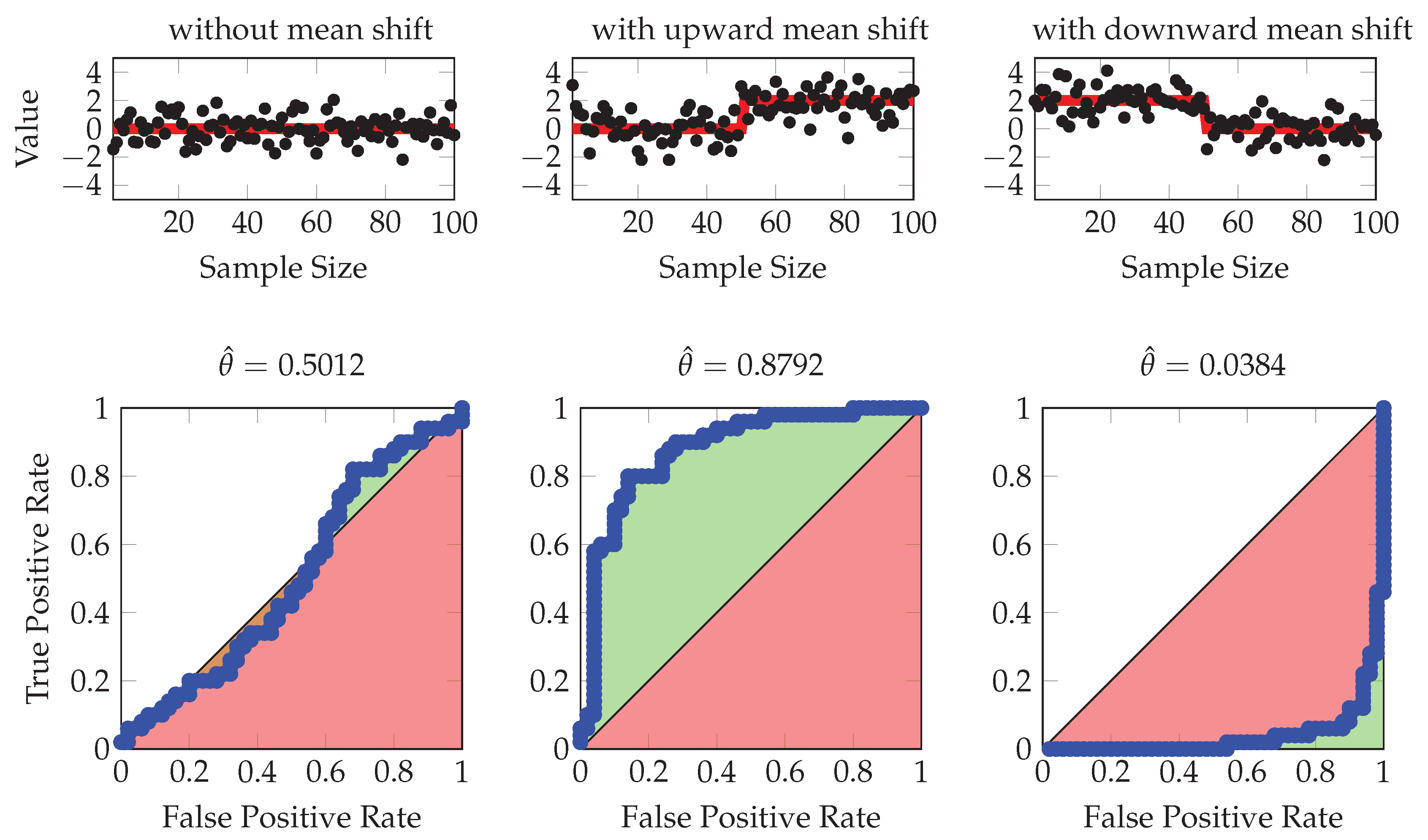
3. AUC Statistics for Change Point with Abrupt Mean Shift

In this section, we use AUC as the statistic to detect the change point. Specifically, the change point detection algorithm can be divided into two stages. In the first stage, the sample data is processed by two sliding windows. The statistic is indirectly obtained by calculating the data sequence in the windows according to the definition of AUC. It can be proved that our algorithm is optimal when the two adjacent windows have the same size. In the second stage for change point analysis, the method of hypothesis testing is used to set a threshold to determine the potential change point. To reduce false alarms, parameter K is used to remove the false alarm interval.

3.1. AUC Statistics from Symmetric Sliding Windows

We consider the data model in Equation (1) with Assumptions 1 and 2. The two-sided two-sample MWUS is used for change point detection. Let $X={\left\{S_i\right\}}_{i=k-m}^k$ and $Y={\left\{S_j\right\}}_{j=k+1}^{k+n}$ are derived from a continuous i.i.d. samples $S_T$. The statistic for potential change points can be expressed as follows:

$${\widehat{\theta }}_k=\frac{1}{mn}\sum _{i=k-m+1}^k\sum _{j=k+1}^{k+n}\mathcal{I}(S_i>S_j)$$

(2)

where $\mathcal{I}(·)$ is the indicator function defined in (1), and $T-n>k>m$. As pointed out by Hanley et al. [25], ${\widehat{\theta }}_k$ is equal to AUC that represents the probability of $X>Y$. This equivalence relationship enables us to call the change point statistics as AUC. In the following, we simply write ${\widehat{\theta }}_k$ as $\widehat{\theta }$ for notational convenience.

Assume that the positive samples X and negative samples Y have two different distributions, denoted by $F_X$ and $F_Y$, respectively. The test statistic defined in (2) is actually a measure of the difference between $F_X$ and $F_Y$. Figure 1 below illustrates such property of the test statistic. Assume that the first half of the data are negative samples and the second half are positive samples. As shown in the first column of Figure 1, if there is no mean shift in the data, the corresponding test statistic is $\widehat{\theta }=P(X>Y)=0.5$, which means $F_X=F_Y$, i.e., this data exist only one distribution. However, if $F_X\ne F_Y$, which means that the data has two different distributions, the test statistic will significantly deviates from $0.5$. As shown in the second column of Figure 1, when the test statistics are significantly greater than $0.5$, it represents the data has an upward mean shift. On the other hand, as shown in the third column of Figure 1, when the test statistic is significantly less than $0.5$, it means that the data has a downward mean shift.

In order to detect the change point(s) from a data sequence $S_T$, we designed two sliding windows, namely, the positive window X (right) of size m, and negative window Y (left) of size n. That is, $X={\left\{S_i\right\}}_{i=k-m+1}^k$ and $Y={\left\{S_i\right\}}_{i=k+1}^{k+n}$. For each pair of the windows, we can calculate a statistic based on (2). By gradually sliding the two windows along the data, we will obtain a sequence of test statistics. From Lemma 1, we know that when $F_X=F_Y$, i.e., there is no mean shift, the expectation of $\widehat{\theta }$ is $\mathbb{E}(\widehat{\theta })=0.5$. As shown in Figure 2, the test statistic $\widehat{\theta }$ fluctuates around $0.5$ before the change point at $\tau$ entering in the two sliding windows X and Y. However, when the change point begins to enter the positive slide window X, $\widehat{\theta }$ begins to increase. When the change point enters the negative slide window Y, $\widehat{\theta }$ begins to decrease. And $\widehat{\theta }$ returns to around $0.5$ when the change point leaves the two sliding windows. The resultant sequence of $\widehat{\theta }$ thus contains the location information of the change point(s).

In the above procedure of calculating $\widehat{\theta }$, two problems need to be addressed. The first one is: when the length sum $m+n$ is fixed, under what relationship of m and n will the variance of $\widehat{\theta }$ is minimized. The second problem is: how to select the suitable window sizes. We will address the two problems in Theorem 1 below and in Section 3.3, respectively.

Lemma 1.

[26] Let$X={\left\{X_i\right\}}_{i=1}^m$and$Y={\left\{Y_j\right\}}_{j=1}^n$be two i.i.d. samples drawn from two unknown continuous distributions with cumulative distribution functions (cdf)$F_X\left(x\right)$and$F_Y\left(y\right)$, respectively. Then the mean and variance of$\widehat{\theta }$in Equation (2) are:

$$\mathbb{E}(\widehat{\theta })\triangleq \theta =Pr(Y<X)={\int }_{-\infty }^{+\infty }{F}_Y\left(y\right)d{F}_X\left(x\right)$$

(3)

$$\mathbb{V}(\widehat{\theta })=\frac{1}{mn}\{Q_0+(n-1)(Q_1-{\theta }^2)+(m-1)[Q_2-{(1-\theta )}^2]\}$$

(4)

where

$$\begin{array}{cc}\hfill Q_0& =\theta (1-\theta )\hfill \end{array}$$

(5)

$$\begin{array}{cc}\hfill Q_1& =Pr(Y<X\cap Y^{\prime }<X)={\int }_{-\infty }^{+\infty }{F}_Y^2\left(y\right)d{F}_X\left(x\right)\hfill \end{array}$$

(6)

$$\begin{array}{cc}\hfill Q_2& =Pr(X<Y\cap X^{\prime }<Y)={\int }_{-\infty }^{+\infty }{F}_X^2\left(x\right)d{F}_Y\left(y\right)\hfill \end{array}$$

(7)

with$X^{\prime }$and$Y^{\prime }$being the i.i.d copies of X and Y, respectively. Moreover, in the case of null hypothesis, that is,$F_X(·)=F_Y(·)$, the expectation and variance of$\widehat{\theta }$satisfy, respectively,

$$\begin{array}{cc}\hfill \mathbb{E}(\widehat{\theta })& =\frac{1}{2}\hfill \end{array}$$

(8)

$$\begin{array}{cc}\hfill \mathbb{V}(\widehat{\theta })& =\frac{m+n+1}{12mn}\hfill \end{array}$$

(9)

Theorem 1.

Assume that the two adjacent sliding windows contain two i.i.d. data$X={\left\{X_i\right\}}_{i=1}^m$and$Y={\left\{Y_j\right\}}_{j=1}^n$, with continuous cdfs$F_X\left(x\right)$and$F_Y\left(y\right)$, respectively. Assume further that$F_X\left(x\right)$and$F_Y\left(y\right)$are symmetric. Let$N=m+n$be a fixed integer. Define the segmentation factor as$\lambda =m/N$. If there is a mean shift Δ between X and Y, i.e., $F_Y\left(x\right)=F_X(x+\mathsf{\Delta })$, then we have

(i) 

${\int }_{-\infty }^{+\infty }{F}_Y^2\left(x\right)d{F}_X\left(x\right)={\int }_{-\infty }^{+\infty }{(1-F_X\left(x\right))}^{2}d{F}_Y\left(x\right)$

(ii) 

For all of the Δ, the variance of $\widehat{\theta }$ based on X and Y reaches its minimum when $m=n$.

Proof. 

(i).

Denote by $f_x$ and $f_y$ the probability density functions (pdfs) of X and Y, respectively. Since $F_Y\left(x\right)=F_X(x+\mathsf{\Delta })$, it follows that $f_x(x+\mathsf{\Delta })=f_y\left(x\right)$, which is equivalent to $f_x\left(x\right)=f_y(-x-\mathsf{\Delta })$. Therefore $F_Y\left(x\right)=F_X(x+\mathsf{\Delta })$ is equivalent to $F_Y\left(x\right)=1-F_X(-\mathsf{\Delta }-x)$. Hence,

$$\begin{array}{cc}\hfill {\int }_{-\infty }^{+\infty }{F}_Y^2(x)d{F}_X(x)& ={\int }_{-\infty }^{+\infty }{F}_Y^2{f}_x(x)dx\hfill \\ \hfill & ={\int }_{-\infty }^{+\infty }{F}_Y^2(x)f_y(-x-\mathsf{\Delta })dx\hfill \\ \hfill & ={\int }_{-\infty }^{+\infty }{(1-F_X(-x-\mathsf{\Delta }))}^2{f}_y(-x-\mathsf{\Delta })dx\hfill \\ \hfill & ={\int }_{-\infty }^{+\infty }{(1-F_X(x))}^{2}d{F}_Y(x)\hfill \end{array}$$

(10)

(ii).

Given the assumption that $N=m+n$ is fixed, it follows from (4) that

$$\begin{array}{cc}\hfill \mathbb{V}(\widehat{\theta })& =\frac{1}{mn}\{Q_0+(n-1)(Q_1-{\theta }^2)+(m-1)[Q_2-(1-{\theta }^2)]\}\hfill \\ \hfill & =\frac{1}{mn}\{\theta -{\theta }^2-(n-1){\theta }^2-(m-1){(1-\theta )}^2+(n-1)Q_1+(m-1)Q_2\}\hfill \\ \hfill & =\frac{1}{mn}\{\theta -(m+n-1){\theta }^2+(m-1)(2\theta -1+Q_2)+(n-1)Q_1\}\hfill \end{array}$$

(11)

which, along with the result of the above equation, leads to

$$\begin{array}{cc}\hfill 2\theta -1+Q_2& =-1+2{\int }_{-\infty }^{+\infty }{F}_Y\left(y\right)d{F}_X\left(x\right)+{\int }_{-\infty }^{+\infty }{F}_X^2\left(x\right)d{F}_Y\left(y\right)\hfill \\ \hfill & =-1+2(1-{\int }_{-\infty }^{+\infty }{F}_X\left(x\right)d{F}_Y\left(y\right))+{\int }_{-\infty }^{+\infty }{F}_X^2\left(x\right)d{F}_Y\left(y\right)\hfill \\ \hfill & ={\int }_{-\infty }^{+\infty }{(1-F_X\left(x\right))}^{2}d{F}_Y\left(y\right)\hfill \\ \hfill & =Q_1.\hfill \end{array}$$

(12)

Therefore, we have

$$\begin{array}{cc}\hfill \mathbb{V}(\widehat{\theta })& =\frac{1}{mn}\{\theta -(m+n-1){\theta }^2+(m-1)(2\theta -1+Q_2)+(n-1)Q_1\}\hfill \\ \hfill & =\frac{1}{mn}\{\theta -(m+n-1){\theta }^2+(m-1)Q_1+(n-1)Q_1\}\hfill \\ \hfill & =\frac{1}{\lambda (1-\lambda )}\{\theta -(N-1){\theta }^2+(N-2)Q_1\}\hfill \end{array}$$

(13)

which shows that the variance of $\theta$ depends only on the length segmentation factor $\lambda$. It thus follows readily that $\mathbb{V}(\widehat{\theta })$ is minimized when $\lambda =0.5$, or equivalently, $m=n$. ☐

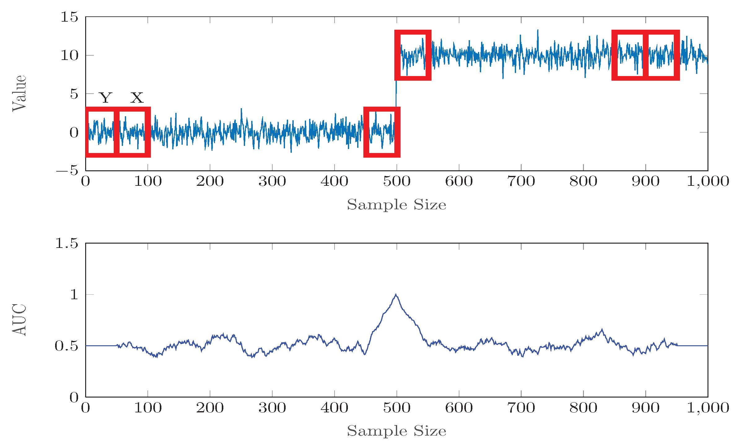
3.2. Change Point Detection with AUC Statistics

In this section, we use hypothesis testing method to determine whether there is any change point in the signal. We also develop a search strategy to identify the location of the change point. The objective of the search strategy is to reduce the false alarm rate. Before going through the detailed steps, we introduce Theorem 2 as follows.

Theorem 2.

[27] Let$X={\left\{X_i\right\}}_{i=1}^m$and$Y={\left\{Y_j\right\}}_{j=1}^n$be i.i.d. random variables having continuous cdfs$F_X\left(x\right)$and$F_Y\left(y\right)$, respectively. Assume that$m⩽n$, and$m/n\to \lambda$when$m,n\to \infty$. Then under the null hypothesis, i.e.,$F_X(·)=F_Y(·)$, the test statistic in Equation (2) follows approximately a Normal distribution$\mathcal{N}(\frac{1}{2},\frac{m+n+1}{12mn})$.

From Lemma 1, we know that when the null hypothesis holds true, the expectation and variance of the $\widehat{\theta }$ equal $E(\widehat{\theta })=0.5$ and $V(\widehat{\theta })=(m+n+1)/12mn$, respectively. Theorem 2 actually means that when $m,n\to \infty$, $W=\frac{1}{\sqrt{V(\widehat{\theta })}}(\widehat{\theta }-0.5)$ converges in distribution to the standard Normal distribution, namely:

$$W=\frac{1}{\sqrt{V(\widehat{\theta })}}(\widehat{\theta }-0.5)\stackrel{d}{\to }\mathcal{N}(0,1)$$

(14)

Note that, to satisfy the requirements of the Theorem 2, literature [28] points out that the sample sizes must be large enough. Sepcifically, $max(m,n)⩾30$ and $m+n⩾40$.

After selecting the suitable window sizes m and n statisfying the requirements in Theorem 2, we can move the two sliding windows forward one data point at a time and calculate the two-sample test statistics. For each window pair, if the test statistic is higher than the threshold determined by a particular significance level, it is considered as a potential change point. Otherwise, the data point is not considered a change point. Mathematically, given the significance level $\alpha$, the test statistics for potential change points satisfy:

$$|W|⩾z_{1-\frac{\alpha }{2}}$$

(15)

where $z_{1-\frac{\alpha }{2}}$ is the percentile $1-\alpha /2$ of standard Normal distribution. When the length of two windows is selected to be $m=n=L_0$, the range of potential change-points can be defined as

$$\widehat{\theta }=\left\{\widehat{\theta }:\widehat{\theta }>0.5+z_{1-\frac{\alpha }{2}}\sqrt{\frac{1}{6L_0}}|\widehat{\theta }<0.5-z_{1-\frac{\alpha }{2}}\sqrt{\frac{1}{6L_0}}\right\}$$

(16)

We define two decision threshold as $thr1$ and $thr2$ from Equation (16). It is obvious that $thr2=1-thr1$. As shown in Figure 3, the upper and lower thresholds are set for the value of $\theta$ to determine whether any potential change point occurs. From the formula $thr1=0.5+z_{1-\frac{\alpha }{2}}\sqrt{\frac{1}{6L_0}}$, we can see that it is related to the significance level and window length. Generally, significance level is set as $\alpha =0.05$. After the significance level is fixed, the threshold value decreases with the increase of the window size. We discuss the problem of window size in Section 3.3.

After determining the decision thresholds, we need the necessary search strategy to determine the location of change point. If the change point is located at the local extrema value of $\widehat{\theta }$ in the data points that continuously exceeds the threshold, it may lead to false alarms. To reduce the chance of false alarm, we define a range parameter K. As shown in Figure 4, if the number of $\widehat{\theta }$ exceeding the threshold is less than K, the point corresponding to the local maximum of $\widehat{\theta }$ is not considered as a change point. On the other hand, if the number of $\widehat{\theta }$ exceeding the threshold is larger than K, the point corresponding to the local maximum of $\widehat{\theta }$ is considered as a change point. As for the selection of K, we will discuss it in Section 3.3. After reducing the false alarm rate, the direction of the change point is determined as follows. If the ultimate extreme value obtained is a local maximum, the data changes upwards; If the ultimate extreme value obtained is a local minimum, the data changes downwards. For example, we define the local maximum of $\theta$ to be:

$$max{\theta }_n^l=max\{{\theta }_j:{\theta }_j>thr1,j=n,n+1\cdots n+l-1,l>K\}$$

(17)

The location of the change point is thus:

$$\tau =arg\underset{n⩽\tau ⩽n+l-1}{max}{\theta }_n^l,l>K$$

(18)

In a parallel manner, we can also define the location of change points whose directions are downward.

3.3. The Window Size and K

Theorem 3.

Assume that the two adjacent sliding windows contain two i.i.d. data$X={\left\{X_i\right\}}_{i=1}^m$and$Y={\left\{Y_j\right\}}_{j=1}^n$, with continuous cdfs$F_X\left(x\right)$and$F_Y\left(y\right)$, and pdfs$f_X\left(x\right)$and$f_Y\left(y\right)$, respectively. Let$N=m+n$be fixed. Define the segmentation factor as$\lambda =m/N$. If there is a mean shift Δ between X and Y, that is, $F_Y\left(x\right)=F_X(x+\mathsf{\Delta })$, the power of test against $\mathsf{\Delta }=0$ is approximately

$$\beta =1-\Phi (z_{\alpha }-\frac{\mathsf{\Delta }}{\tau }\sqrt{\lambda (1-\lambda )N})$$

(19)

at level α. Moreover, if the power β has been determined, the sample size required for the test can be estimated as

$$N=\frac{{(z_{\alpha }-z_{\beta })}^2}{{\mathsf{\Delta }}^2\lambda (1-\lambda )}{\tau }^2$$

(20)

where $\tau ={(\sqrt{12}\int f_X^2\left(x\right)dx)}^{-1}$.

Theorem 3 shows that when $\alpha$, $\beta$ and segmentation factor $\lambda$ are prescribed, the size of the window is related to the mean shift and the distribution under the null hypothesis. That is, as long as the null distribution and the mean shift are determined, the required sample size can be obtained. For example, the null distribution is the standard Normal distribution. When it has a mean shift $\mathsf{\Delta }=1.0$, then $\tau =\sqrt{\frac{\pi }{3}}$. In this case, if $\alpha =0.05$, $\beta =0.95$, and the two windows are symmetric with $\lambda =0.5$, the corresponding sliding window size is at least $m=n=22$. If only the mean shift is changed to $\mathsf{\Delta }=0.5$ while other conditions remain unchanged, the sliding window size is at least $m=n=88$. It should be noted that this theorem has been proved by Lehmann. See [29] for the detailed argument. In addition, when the distribution of null hypothesis is unknown, the sample sizes dependon on $\tau$, which can be estimated by the technique in [30].

According to Equation (19), the test power is affected by both the window sizes and mean shift. We use Monte Carlo method to simulate the stand Normal distribution for 1000 times, so as to observe the influence of window sizes on the accuracy of change point detection under different mean shifts. In this simulation study, the data sequence contains $T=1000$ data points, and the change point is at the location of $t^{*}=500$. As shown in Figure 5, in the case of a single change point, the accuracy of detection increases with the increase of window sizes within a certain range. Furthermore, when the window size is fixed, it is observed in Figure 5 that, the smaller the shift $\mathsf{\Delta }$ is, the more likely the data is to be interfered by noise, and the more difficult the change point is to be detected. On the other hand, the larger the shift is, the higher the accuracy of the algorithm is. When the shift increases to a certain value, the accuracy of the alogrithm tends to 100%. However, in the case of multiple change points detection, the size of the sliding windows cannot be too large. When the size of the windows is larger than the interval between two neighboring change points, the detection results will become unacceptable. Therefore, care should be taken when selecting the size of the sliding windows in practice.

Another problem is the choice of K. Cunen et al. [31] proposed some methods for the confidence interval distribution of change points. Inspired by this method, we take into account he interval length distribution of test statistics beyond the set threshold when selecting the magnitude of K. We define ${\theta }_{0,j}$ and ${\theta }_{1,j}$ as the obtained test sequences in the cases of change-point absence and change-point presence, respectively. In the former case (null case), the longest interval beyond the threshold is defined as $K_0^{max}$; while in the latter case (there is an upward mean shift), the interval where the truce change point $t^{*}$ locates is defined $K_1^{*}$. They are expressed respectively as:

$$K_0^{max}=max\{l:{\theta }_{0,n}^l>thr1\cup {\theta }_{0,n}^l<1-thr1,{\theta }_{0,n}^l={\theta }_{0,j},j=n,n+1,\cdots n+l-1\}$$

(21)

$$K_1^{*}=\{l:t^{*}\in [n,n+l-1]\cap {\theta }_{1,n}^l>thr1,{\theta }_{1,n}^l={\theta }_{1,j},j=n,n+1,\cdots n+l-1\}$$

(22)

Figure 6 illustrates the idea of how to choose a suitable K for Normal distribution, Log-normal distribution and Cauchy distribution. The window size is set to be $m=n=50$, and the mean shifts are set to be $0.75,1.0,2.0$, respectively. From the distributions of $K_0^{max}$ and $K_1^{*}$ shown in Figure 6, it is observed that, (1) when $shift=0.75$, the optimal K corresponding to the Normal and Log-normal distribution is within $[20,25]$, while the selection of K for the Cauchy distribution is meaningless; (2) when $shift=1.0$, the optimal K corresponding to the Normal and Log-normal distribution is within $[30,35]$, while the selection of K for the Cauchy distribution is $[25,30]$; (3) when $shift=2.0$, the optimal K corresponding to the Normal and Log-normal distribution is within $[40,45]$, while the selection of K for the Cauchy distribution is $[25,30]$; (4) if the value of the shift continues to increase, the optimal K of the three distributions will be all stable at 50. Based on the above observations, we suggest that the selection interval of K is $[15,50]$ when the symmetrical window size is 50.

4. Comparative Studies and Analysis

In this section, we evaluate the performance of our algorithm under various scenarios based on the MATLAB platform. We first compare our method with the classical algorithms by Monte Carlo simulations with respect to three distributions in the scenario of single change point detection. We also apply our method to the case of multiple change points detection based on artificial and real data sets.

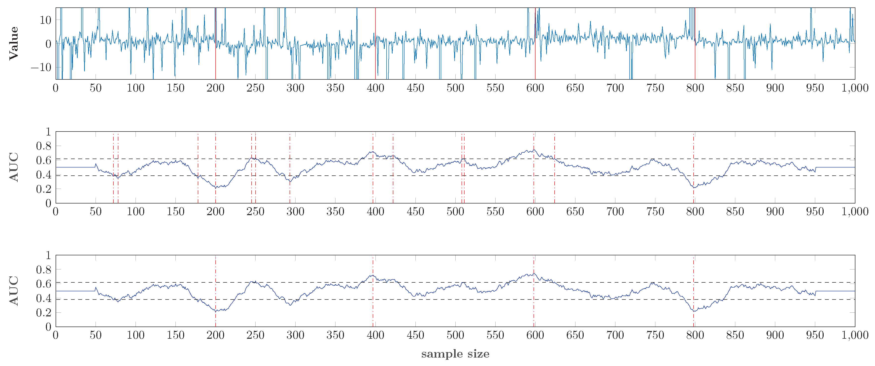
4.1. Comparative Results for Single Change Point Detection

In order to evaluate performance, we employ the index of accuracy as a figure of merit. Specifically, if the detected change point is sufficiently close to a real change point, i.e., ${\widehat{t}}^{*}\in [t^{*}-20,t^{*}+20]$, where $t^{*}$ is the true location of change point, the point at ${\widehat{t}}^{*}$ is considered to be a correct detection. According to the above rule, the accuracy is computed by

$$\begin{array}{cc}\hfill N_{correct}& =\sum _{i=1}^w\mathcal{I}\left\{\right|{\widehat{t}}_i^{*}-t_i^{*}|\le 20\}\hfill \end{array}$$

(23)

$$\begin{array}{cc}\hfill \mathit{accuracy}& =\frac{N_{correct}}{w}\hfill \end{array}$$

(24)

where w is the number of trials, and $N_{correct}$ is the number of correct detections.

In the following simulation studies, the data length T in Equation (1) is set to be $T=1000$. The abrupt change location is set at $t^{*}=500$, the mean shifts at $t^{*}=500$ are $\mathsf{\Delta }=[0.25,0.50,0.75,1.00,1.25,1.50,1.75,2.00]$, respectively. The sliding window size was set to be $m=n=50$. We use a constant signal with ${\mu }_0=0$ and corrupt it with three types of i.i.d. noise. The models of noise are:

• Model 1: Normal distribution

  $$e\left(t\right)\sim \mathcal{N}(0,1),1\le t\le T$$
• Model 2: Log normal distribution

  $$log\left(e\right(t\left)\right)\sim \mathcal{N}(0,1),1\le t\le T$$
• Model 3: Standard Cauchy distribution

  $$e\left(t\right)\sim \mathcal{C}(1,0),1\le t\le T$$

Given the above conditions, the data used in single change point detection can thus be expressed as

$$S\left(t\right)=\mathsf{\Delta }\ast \mathcal{I}\left(500⩽t⩽1000\right)+e\left(t\right),t=1,2,\dots ,1000$$

(25)

Figure 7 shows the comparative results of our method with HQK [22] and RuLSIF [23], where the number of trials $w=1000$. It is observed that, (1) under Model 1, i.e., the noise is Normal, our method performs only sightly worst than HQK and RuLSIF (Figure 7a,b); (2) under Model 2, i.e., the noise is Log-normal, our method outperforms HQK outperforms RuLSIF, especially for $\mathsf{\Delta }<0.75$ (Figure 7c,d); (3) under Model 3, i.e., the noise is Cauchy, the performance of our method is much better than HQK and RuLSIF, manifesting the robustness of our method against noise with strong spiky patterns (Figure 7e,f). For the detailed detection accuracis, see

Table A1. Experiment Performance.

Shift ($\mathbf{\Delta }$)	Normal Distribution			Log Normal Distribution			Cauchy Distribution
	AUC	RuLSIF	HQK	AUC	RuLSIF	HQk	AUC	RuLSIF	HQK
0	0.047	0.0	0.014	0.052	0.0	0.015	0.058	0.0	0.006
0.25	0.188	0.0	0.391	0.244	0.0	0.123	0.077	0.0	0.009
0.5	0.496	0.0	0.808	0.605	0.0	0.366	0.180	0.0	0.012
0.75	0.778	1	0.939	0.867	0.0	0.604	0.380	0.0	0.012
1	0.954	1	0.988	0.946	0.0	0.772	0.561	0.0	0.018
1.25	0.989	1	0.998	0.972	1	0.882	0.724	0.0	0.027
1.50	0.998	1	1	0.986	1	0.928	0.839	0.0	0.050
1.75	1	1	1	0.995	1	0.964	0.901	0.0	0.040
2.00	1	1	1	0.999	1	0.965	0.932	0.0	0.057

.

4.2. Multiple Change Points Detection

Besides the ability of detecting single change point, our method is also capable of detecting multiple change points. Similar to the previous settings, we also use a sequence with 1000 data points. The locations of the change points are $t_1^{*}=200$, $t_2^{*}=400$, $t_3^{*}=600$, $t_4^{*}=800$, with corresponding mean shifts being $[{\mathsf{\Delta }}_1,{\mathsf{\Delta }}_2,{\mathsf{\Delta }}_3,{\mathsf{\Delta }}_4]=[-1,1,1,-1]$. The window size is $m=n=50$. The maximum of 20 or more data points that continuously exceed the threshold ($K=20$) is considered as the location estimates of the change points. The detection results with respect to Model 1 to Model 3 are depicted in Figure 8, Figure 9 and Figure 10, respectively.

Figure 8 depicts the detection precedure under Model 1, where the noise follows the Normal distribution. The top panel shows the data with red lines indicating the real locations of the change points. In the middle panel are the local extrema without the process of false alarm rejection. It can be seen that 10 change points are detected, 6 of which are false alarms. The bottom panel shows finally detected change points after the false-alarm rejection procedure. The final detected change points are located at $199,400,599,800$, respectively, very close to the corresponding true locations at $t_1^{*}=200$, $t_2^{*}=400$, $t_3^{*}=600$, $t_4^{*}=800$. Figure 9 depicts the detection precedure under Model 2, where the noise follows the Log normal distribution. Similar to that in Figure 8, The final detected change points are located at $200,400,602,805$, respectively, very close to the corresponding true locations at $t_1^{*}=200$, $t_2^{*}=400$, $t_3^{*}=600$, $t_4^{*}=800$. Figure 10 depicts the detection precedure under Model 3, where the noise follows the Cauchy distribution. The final detected change points are located at $200,398,599,799$, respectively, very close to the corresponding true locations at $t_1^{*}=200$, $t_2^{*}=400$, $t_3^{*}=600$, $t_4^{*}=800$.

The detection results in Figure 8, Figure 9 and Figure 10, respectively, verify the ability of our method in detecting multiple change points when the noise follows various distributions.

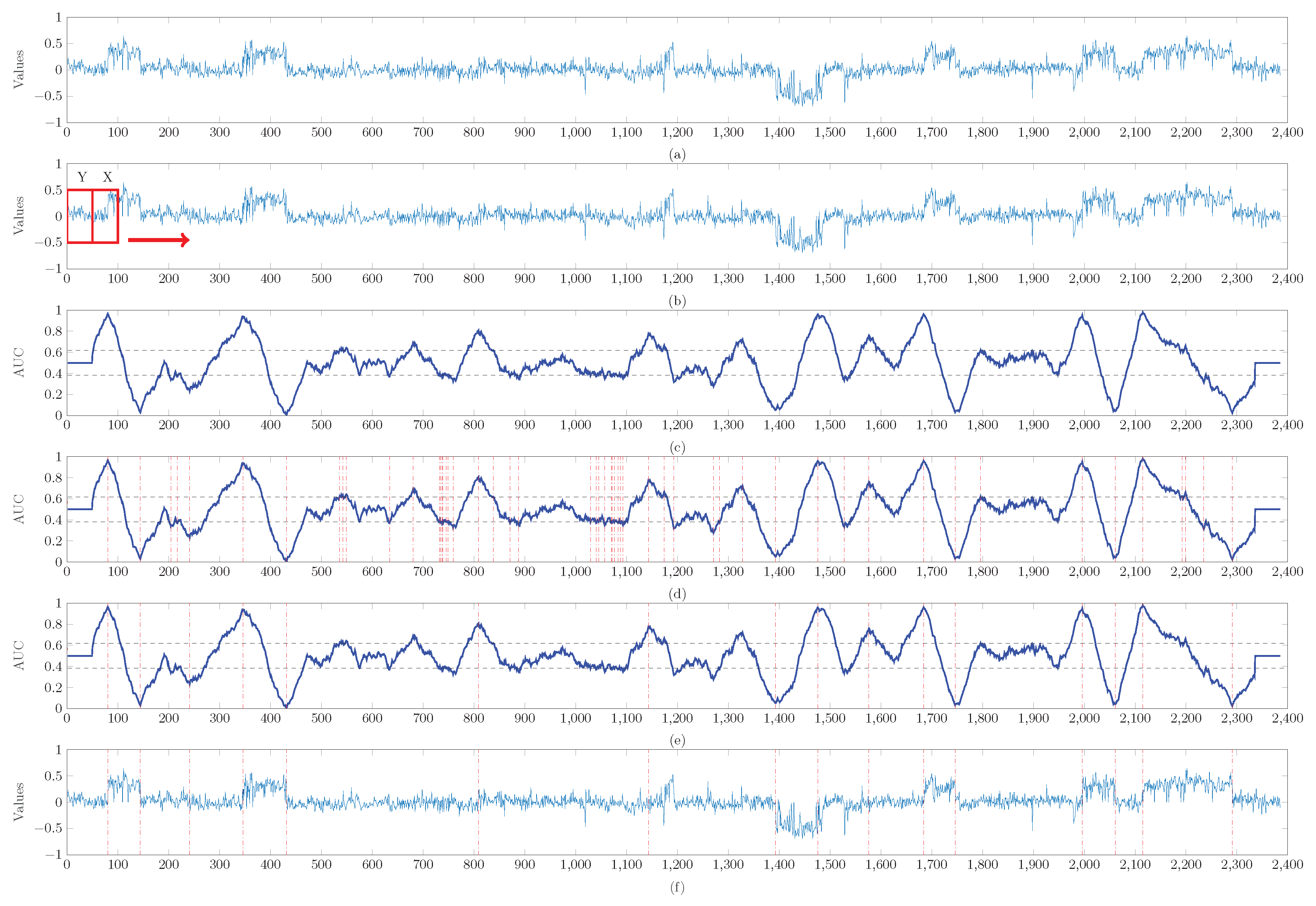
4.3. An Application to Real Data Set

To gain further insight of our method, we apply it to detecting multiple change points based on a real genetric data set [32] (http://microarrays.curie.fr/publications/oncologie_moleculaire/bladder_TCM/). It is a sample of 57 patients with bladder cancer and contains the log2ratio, GNL status (Gain/−1, normal/0 or loss/1) and outlier status of all 2385 BAC clones. It should be noted that these data are the result of normalization of the original data on a logarithmic scale.

We need to process the missing values in the data set before applying our method. Following the work in [33], we remove all sequences with missing values greater than 7%. After screening, we retain the genetic data of 41 samples and set the missing value of these samples to zero. We randomly select the 40th sample as an example in this study.

Figure 11 ($K=30$) shows the procedure as well as the results of our algorithm: (a) the pre-processed genetic data; (b) demo of the sliding windows ($m=n=50$); (c) the test statistics and decision thresholds; (d) the detected local extrema with false alarms; (e) the final change points obtained after false alarm rejection; and (f) the the original data marked with the location of the detected change points. As can be seen, our method detects 16 change points, among which nine mutate upward and seven mutate downward. These 16 change points are not missing, but there are two change points that are false alarms and are not technically change points. They are located near 800 and 1600 respectively.

5. Conclusions

In this paper, we propose an AUC-based algorithm for the detection of change point(s) with mean shift. Theoretical derivations and numerical results showed that our method has the following advantages, including (1) it is a non-parametric method possessing the distribution free property, (2) it performs comparably well with two state-of-the-art methods when the noise is Normal, (3) it performs better than the other two methods when the noise is impulsive (Log-normal and Cauchy distributions), (4) it can be applied to detecting of multiple change points, and (5) it is capable of detecting the direction of mean shift. Having the above advantages, the proposed method can play a complementary role to other methods in the literature, especially when the noise distribution, deviating significantly from Normal, exhibits an impulsive manner (such as Cauchy noise).

References

1. Nikovski, D.; Jain, A. Memory-based algorithms for abrupt change detection in sensor data streams. In Proceedings of the 2007 5th IEEE International Conference on Industrial Informatics, Vienna, Austria, 23–27 July 2007; Volume 1, pp. 547–552. [Google Scholar]
2. Nikovski, D.; Jain, A. Fast adaptive algorithms for abrupt change detection. Mach. Learn. 2010, 79, 283–306. [Google Scholar] [CrossRef] [Green Version]
3. Goswami, B.; Boers, N.; Rheinwalt, A.; Marwan, N.; Heitzig, J.; Breitenbach, S.F.; Kurths, J. Abrupt transitions in time series with uncertainties. Nat. Commun. 2018, 9, 48. [Google Scholar] [CrossRef] [PubMed]
4. Staniszewski, M.; Skorupa, A.; Boguszewicz, Ł.; Sokół, M.; Polański, A. Quality Control Procedure Based on Partitioning of NMR Time Series. Sensors 2018, 18, 792. [Google Scholar] [CrossRef] [PubMed] [Green Version]
5. Xie, Y.; Siegmund, D. Sequential multi-sensor change-point detection. Ann. Stat. 2013, 41, 670–692. [Google Scholar] [CrossRef]
6. Wang, H.; Zhang, D.; Shin, K.G. Change-point monitoring for the detection of DoS attacks. IEEE Trans. Dependable Secur. Comput. 2004, 1, 193–208. [Google Scholar] [CrossRef]
7. Oudre, L.; Lung-Yut-Fong, A.; Bianchi, P. Segmentation of accelerometer signals recorded during continuous treadmill walking. In Proceedings of the IEEE 2011 19th European Signal Processing Conference, Barcelona, Spain, 29 August–2 September 2011; pp. 1564–1568. [Google Scholar]
8. Gan, F. An optimal design of CUSUM control charts for binomial counts. J. Appl. Stat. 1993, 20, 445–460. [Google Scholar] [CrossRef]
9. Jiang, W.; Shu, L.; Tsui, K.L. Weighted CUSUM control charts for monitoring Poisson processes with varying sample sizes. J. Qual. Technol. 2011, 43, 346–362. [Google Scholar] [CrossRef]
10. Steiner, S.H.; Mackay, R.J. Monitoring processes with highly censored data. J. Qual. Technol. 2000, 32, 199–208. [Google Scholar] [CrossRef] [Green Version]
11. Noura, A.; Read, K. Proportional hazards changepoint models in survival analysis. J. R. Stat. Soc. Ser. C Appl. Stat. 1990, 39, 241–253. [Google Scholar] [CrossRef]
12. Gijbels, I.; Goderniaux, A.C. Bandwidth selection for changepoint estimation in nonparametric regression. Technometrics 2004, 46, 76–86. [Google Scholar] [CrossRef]
13. Oh, K.J.; Moon, M.S.; Kim, T.Y. Variance change point detection via artificial neural networks for data separation. Neurocomputing 2005, 68, 239–250. [Google Scholar] [CrossRef]
14. Goldenshluger, A.; Tsybakov, A.; Zeevi, A. Optimal change-point estimation from indirect observations. Ann. Stat. 2006, 34, 350–372. [Google Scholar] [CrossRef] [Green Version]
15. Wang, Z.F.; Wu, Y.H.; Zhao, L.C. Change-point estimation for censored regression model. Sci. China Ser. A Math. 2007, 50, 63–72. [Google Scholar] [CrossRef]
16. Pettitt, A. A non-parametric approach to the change-point problem. J. R. Stat. Soc. Ser. C Appl. Stat. 1979, 28, 126–135. [Google Scholar] [CrossRef]
17. Hawkins, D.M.; Deng, Q. A nonparametric change-point control chart. J. Qual. Technol. 2010, 42, 165–173. [Google Scholar] [CrossRef]
18. Ross, G.J.; Tasoulis, D.K.; Adams, N.M. Nonparametric monitoring of data streams for changes in location and scale. Technometrics 2011, 53, 379–389. [Google Scholar] [CrossRef]
19. Zou, C.; Tsung, F.; Wang, Z. Monitoring profiles based on nonparametric regression methods. Technometrics 2008, 50, 512–526. [Google Scholar] [CrossRef]
20. Qiu, P.; Zou, C.; Wang, Z. Nonparametric profile monitoring by mixed effects modeling. Technometrics 2010, 52, 265–277. [Google Scholar] [CrossRef]
21. Keriven, N.; Garreau, D.; Poli, I. NEWMA: A new method for scalable model-free online change-point detection. arXiv 2018, arXiv:1805.08061. [Google Scholar]
22. Hawkins, D.M.; Qiu, P.; Kang, C.W. The changepoint model for statistical process control. J. Qual. Technol. 2003, 35, 355–366. [Google Scholar] [CrossRef]
23. Liu, S.; Yamada, M.; Collier, N.; Sugiyama, M. Change-point detection in time-series data by relative density-ratio estimation. Neural Netw. 2013, 43, 72–83. [Google Scholar] [CrossRef] [PubMed] [Green Version]
24. Kanamori, T.; Hido, S.; Sugiyama, M. A least-squares approach to direct importance estimation. J. Mach. Learn. Res. 2009, 10, 1391–1445. [Google Scholar]
25. Hanley, J.A.; McNeil, B.J. The meaning and use of the area under a receiver operating characteristic (ROC) curve. Radiology 1982, 143, 29–36. [Google Scholar] [CrossRef] [PubMed] [Green Version]
26. Xu, W.; Dai, J.; Hung, Y.; Wang, Q. Estimating the area under a receiver operating characteristic (ROC) curve: Parametric and nonparametric ways. Signal Process. 2013, 93, 3111–3123. [Google Scholar] [CrossRef]
27. Hettmansperger, T.P.; McKean, J.W. Robust Nonparametric Statistical Methods; CRC Press: Boca Raton, FL, USA, 2010. [Google Scholar]
28. Mason, S.J.; Graham, N.E. Areas beneath the relative operating characteristics (ROC) and relative operating levels (ROL) curves: Statistical significance and interpretation. Q. J. R. Meteorol. Soc. A J. Atmos. Sci. Appl. Meteorol. Phys. Oceanogr. 2002, 128, 2145–2166. [Google Scholar] [CrossRef]
29. Lehmann, E.L. Elements of Large-Sample Theory; Springer: New York, NY, USA, 1999. [Google Scholar]
30. Schweder, T. Window estimation of the asymptotic variance of rank estimators of location. Scand. J. Stat. 1975, 113–126. [Google Scholar]
31. Cunen, C.; Hermansen, G.; Hjort, N.L. Confidence distributions for change-points and regime shifts. J. Stat. Plan. Inference 2018, 195, 14–34. [Google Scholar] [CrossRef] [Green Version]
32. Nicolas, S.; Céline, V.; Fabien, R.; Isabelle, B.P.; Medina Sixtina Gil Diez, D.; Rick, S.; Yann, D.R.; Paul, E.; Andrew, C.; Carolyn, S. Regional copy number-independent deregulation of transcription in cancer. Nat. Genet. 2006, 38, 1386–1396. [Google Scholar]
33. Matteson, D.S.; James, N.A. A nonparametric approach for multiple change point analysis of multivariate data. J. Am. Stat. Assoc. 2014, 109, 334–345. [Google Scholar] [CrossRef] [Green Version]
Figure 1. Probabilistic meaning of the test statistic. From left to right, the first column is the data without mean shift and its corresponding θ ^ = 0.5012 ; the second column is the data with upward mean shift and its corresponding θ ^ = 0.8792 ; the third column is the data with the downward mean shift and its corresponding θ ^ = 0.0384 .
Symmetry 12 00599 g001
Figure 2. Two continuous sliding windows slide to calculate the test statistics one data point by one data point to obtain a continuous test sequence.
Symmetry 12 00599 g002
Figure 3. Thresholds are determined via the confidence level of the null hypothesis distribution.
Symmetry 12 00599 g003
Figure 4. Demonstration of data points that continuously exceed the threshold value of K.
Symmetry 12 00599 g004
Figure 5. The effect of window size on the performance of the proposed algorithm.
Symmetry 12 00599 g005
Figure 6. The distribution of the maximum value of K under the null hypothesis (red) and the distribution of the interval length of the true change point (blue).
Symmetry 12 00599 g006
Figure 7. Comparative results with respect to noises with (a) Normal distribution, (c) Log normal distribution, and (e) Cauchy distribution. (b) Accuracy under Normal distribution.(d) Accuracy under Log normal distribution. (f) Accuracy under Cauchy distribution.
Symmetry 12 00599 g007
Figure 8. (Top): Data with Normal distribution. The red lines are located at the positions of four real change points; (Middle): test statistics with decision thresholds, and the dotted red lines correspond the local extrema without false alarm reduction; (Bottom): the dotted red lines indicate the final detected locations for the change points.
Symmetry 12 00599 g008
Figure 9. (Top): Data with Log normal distribution. TThe red lines are located at the positions of four real change points; (Middle): test statistics with decision thresholds, and the dotted red lines correspond the local extrema without false alarm reduction; (Bottom): the dotted red lines indicate the final detected locations for the change points.
Symmetry 12 00599 g009
Figure 10. (Top): Data with Cauchy distribution. The red lines are located at the positions of four real change points; (Middle):test statistics with decision thresholds, and the dotted red lines correspond the local extrema without false alarm reduction; (Bottom): the dotted red lines indicate the final detected locations for the change points.
Symmetry 12 00599 g010
Figure 11. The procedure of change point detecion on real genetic data. (a) The pre-processed genetic data. (b) Demo of the sliding windows with m = n = 50 . (c) The test sequence and decision thresholds. (d) Detected change points with false alarms. (e) Final change points after false alarm rejection. (f) Original data marked with the locations of the finally detected change points.
Symmetry 12 00599 g011