1. Introduction
The present work is motivated mainly by problems arising in identification and modelling of biological systems, although its results are applicable in other fields. We consider nonlinear dynamic models defined by ordinary differential equations. This framework is sufficiently powerful to model a wide range of biological processes, from intracellular networks to whole ecosystems, with the appropriate level of detail.
When compared to other applications, biological models often pose specific challenges due to the combination of nonlinearity, uncertainty about the underlying system, and experimental limitations regarding the possibility of perturbations and of measurements [
1]. These features make the identification of biological models particularly challenging, and call for new methodological developments and computational tools. Indeed, many theoretical advances in nonlinear systems identification have been motivated by biological problems, even though the type of problems being considered are often common to other scientific areas, which makes the resulting methodologies generally applicable [
2,
3]. An example is the study of structural identifiability, a property that was introduced in the context of physiological modelling [
4] and has since then been adopted in many scientific and technological areas; since its study is of particular interest for biological models, many related theoretical developments have been motivated by biological problems [
5,
6,
7]. Structural identifiability refers to the possibility of inferring the values of the unknown (constant) parameters in the model equations from observations (measurements) of the model output. It is closely related to—and in fact can be considered a particular case of—another property, observability, which describes the possibility of determining the (time-varying) state variables of the model [
8]. By considering the parameters as constant state variables, structural (local) identifiability amounts to observability (In accordance with the usual terminology, we speak of structural identifiability to distinguish it from practical identifiability. The latter quantifies the uncertainty in parameter values taking into account the information content of the available data, which may be limited due to experimental errors or low sampling rates. We also specify that it is structural local identifiability to distinguish it from structural global identifiability. Although observability is also a structural local property, for historical reasons we do not add those adjectives to its name, and refer to it simply as observability.).
The cause of lack of structural identifiability or observability can be traced back to the existence of symmetries in the model equations. In the present work we use Lie’s theory on symmetry analysis of differential equations [
9,
10,
11]. It has been shown [
12] that the existence of Lie symmetries is equivalent to the existence of similarity transformations, i.e., transformations of parameters and variables that leave the output(s) unchanged [
13,
14]. This means that the existence of symmetries amounts to lack of structural identifiability and/or observability.
Here we revisit a method for finding symmetries by transforming rational expressions into linear systems [
15]. Determining the existence of symmetries in a model is a way of analysing its structural identifiability and observability. Furthermore, if symmetries exist, their mathematical expressions provide information about the relationships between model variables that cause loss of identifiability and/or observability. One way of exploiting these insights is by fixing one or more parameters involved in a symmetry, in order to render the remaining ones identifiable. Another way is by using the symmetry-breaking transformations to reformulate the model, applying the transformations so that the symmetries disappear and the new model is identifiable and observable. In this paper, we extend the method by enabling it to provide symmetry-breaking transformations, which allows for a semi-automatic model reformulation that renders a non-observable model observable. Thus, the approach can be used not only for characterizing the identifiability and observability of a model, but also for suggesting alternative reformulations if the original model does not possess those properties. We illustrate the usefulness and applicability of this approach in biological applications with four models of biochemical processes. Furthermore, we provide an implementation of the methodology as part of a new version of the STRIKE-GOLDD software
https://github.com/afvillaverde/strike-goldd_2.1. STRIKE-GOLDD is a MATLAB toolbox that analyses structural identifiability and observability using a differential geometry approach [
16,
17,
18].
The organization of this paper is as follows: we begin by providing an overview of the methodological aspects in
Section 2. Then we illustrate its application to a number of modelling problems in
Section 3. Finally, we discuss the implications and provide some conclusions in
Section 4.
2. Methods
2.1. Structural Identifiability and Observability
For the study of observability and identifiability we consider the following type of models:
with a parameter vector
, known input functions
, unknown input functions
, state vector
, output vector
and,
f and
g vectors constituted by analytical functions. From this point on, the time dependency will be omitted to simplify the notation.
Definition 1. A parameter , denoting the ith component, of the model is structurally locally identifiable (SLI) if for almost any parameter vector there is a neighbourhood in which the following relation holds: If the above definition does not hold for any neighbourhood of , is structurally unidentifiable (SU). If all model parameters are SLI, the model is SLI too. Otherwise, the model is SU.
Similarly, the observability of a state can be defined as:
Definition 2. Given an output vector and a known input vector , the state is observable if it can be determined from and in the interval , where is a finite time. Otherwise, it is unobservable.
A model is observable if all states are observable. The same definition applies to the unknown entries vector but instead of observable, it is called reconstructible.
The term Full Input-State-Parameter Observability (FISPO) has been recently proposed [
8] to refer to a model that is observable, identifiable and reconstructible. Its formal definition is given by:
Definition 3. Given the model (1), the unknown quantities vector is considered . Denoting each component of z in time τ as with , for a finite . The model is FISPO if the following condition holds: Observability and identifiability can be studied jointly if the parameters are considered as constant states. Thus, the observability of these states is equivalent to the local structural identifiability. Therefore, the augmented state vector is [
18]:
In this way, the model (
1) is transformed into:
To determine the observability of a model it is necessary to calculate the nonlinear observability matrix using Lie derivatives. In the case of time-dependent entries, i.e., , Lie derivatives are computed as follows:
Definition 4. The first order Lie derivative of with respect to is:where is the jth derivative of u. For higher orders, , the calculation is done through a recursive procedure: The observability-identifiability matrix of the previous model is defined as:
Theorem 1. Nonlinear Observability-Identifiability Condition (OIC). If the model (5) satisfies , with given by (8), where is a point in the augmented state space, then the model is locally observable and locally structurally identifiable in a neighbourhood of [18]. If the OIC is not fulfilled, there is at least one unobservable (respectively, unidentifiable) state (respectively, parameter). In that case, full observability may sometimes be achieved by measuring more variables or functions. However, sometimes it is not possible to perform more measurements due to the characteristics of the experiments.
2.2. Lie Symmetries and Structural Unidentifiability
Yates et al. [
12] showed that the existence of Lie symmetries entails the existence of similarity transformations, and therefore denotes lack of structural identifiability [
13,
14]. Similarity transformations allow the existence of parameters and variables transformations that leave the output(s) unchanged.
In Lie algebra, similarity transformations are one-parameter Lie group morphisms that map a solution of the differential equation onto themselves in terms of state variables. There are an infinite number of ways to represent this morphism, however the representation is unique when independent variables are fixed. The uniqueness of representation is a key property for the purpose of implementing the algorithm.
The expression of the one-parameter Lie group of transformations is:
Expanding the above expression in some neighborhood of
:
where
is the infinitesimal of (
9) and
is the infinitesimal transformation of the Lie group of transformations.
Definition 5 ([
9])
. The infinitesimal generator of the one-parameter Lie group of transformations is the differential operator:where ▽
defines the gradient Theorem 2. First Fundamental Theorem of Lie [9]. Given an initial value problem (IVP) for a system of first-order ODEs:The Lie group of transformations (9) is equivalent to the above IVP with the parametrization :where is the law of composition and denotes the inverse element to ε. The above theorem shows how infinitesimal transformations contain the essential information that determines the uniparametric Lie group of transformations. From Theorem (2) and without loss of generality, it is assumed that the Lie group of transformations has as its law of composition
with
and
[
9]. Therefore, the uniparametric Lie group of transformations (
9) is rewritten, in terms of its infinitesimals
, as:
The above expression defines an Initial Value Problem (IVP) for the Lie group of transformations in terms of its infinitesimals generators.
The exponential parametrization of the Lie group around the identity is:
Theorem 3 ([
9])
. The one-parameter Lie group of transformations (9) is equivalent to:where X is given by (12) and with . For a more detailed background, we refer the reader to [
9,
11].
2.2.1. Computing Symmetries
Let us consider the same ODE system as in (
1). The state vector will be augmented with parameters and unknown inputs, as mentioned earlier:
where
.
We will study three different infinitesimals. Considering , as the maximum degree for polynomials and unknown constants to determine, the expressions of infinitesimals are:
The derivative of infinitesimal generators is also defined, so that it can act on the
:
where
Using the above formulation for infinitesimals generators, the following explicit criterion for admittance of a Lie group of transformations is obtained:
Theorem 4 ([
9,
10])
. The system of ordinary differential equations admits a one-parameter Lie group of transformations defined by the infinitesimal generator (12) if and only if: Applying the previous theorem to the initial system (
1), we obtain an explicit criterion:
An admitted Lie symmetry is a continuous group of transformations
X such that the observation (observed datum) is unchanged:
The output map should not be modified. The above system defines a system of partial differential equations. If we consider the rational form of
and
:
then, the system of PDEs (
24) is converted into a system of ODEs.
There are different expressions of (
24) depending on the infinitesimal generator:
Each of these equations can be reordered based on the combinations among the components of
x. Let
r be a vector containing all
:
The coefficients
are linear in
r and its matrix form expression allows to reformulate condition (
26) and (
27) into:
The problem of finding symmetries is equivalent to solving a linear system of equations with numeric entries. However, C is a non-square matrix and, in order to find all the solutions, it is necessary to compute its kernel. It is possible that the obtained solutions are not independent of each other, as a result of linear combinations or multiplication by ; for this reason, we will only consider solutions that are independent of each other and in their greatest degree of simplification.
The next step is to build the expression of
with the infinitesimal generators as in Theorem (3). When the infinitesimal transformation is given by powers of the variable, the exact transformation is known and it is classified as “elementary”. Some examples are:
The most common types of symmetries in biochemical models are translation and scaling. However, those elementary transformations cover only a part of the possible symmetries that a model can contain. The others must be calculated using Lie series or solving the IVP (
16).
It is possible to maximize the number of elementary transformations given by an infinitesimal generator before applying Lie series. This process starts by searching for all parameter combinations that forbid an elementary transformation, and dividing the initial infinitesimal generator by them. Each new infinitesimal generator provides a number of elementary transformations that can be greater than, lower than or equal to the initial one. Maximizing the total amount, we will obtain an infinitesimal generator that provides the largest possible number of elementary transformations.
2.2.2. Initial Conditions
The definition of a dynamic model may include specific initial conditions (ICS), which can be numeric, parametric (known or unknown) or a combination of both [
19,
20]. Perturbations in ICS must produce changes in the output
for the model to be observable.
If the symmetries are studied without taking into account the ICS, it may happen that the generators do not fulfill them. It is important to consider only the generators that satisfy the ICS [
19]; by including them as output vectors, a symmetry is admitted by the system if and only if:
where
are the ICS (parametric, numerical or a combination of both). Expanding the above equation:
Considering the rational form of
:
Expression (
31) is reformulated as follow:
This new restriction allows us to consider only those symmetries that fulfill the initial conditions, and provides a tool for study the influence of them.
2.3. Implementation
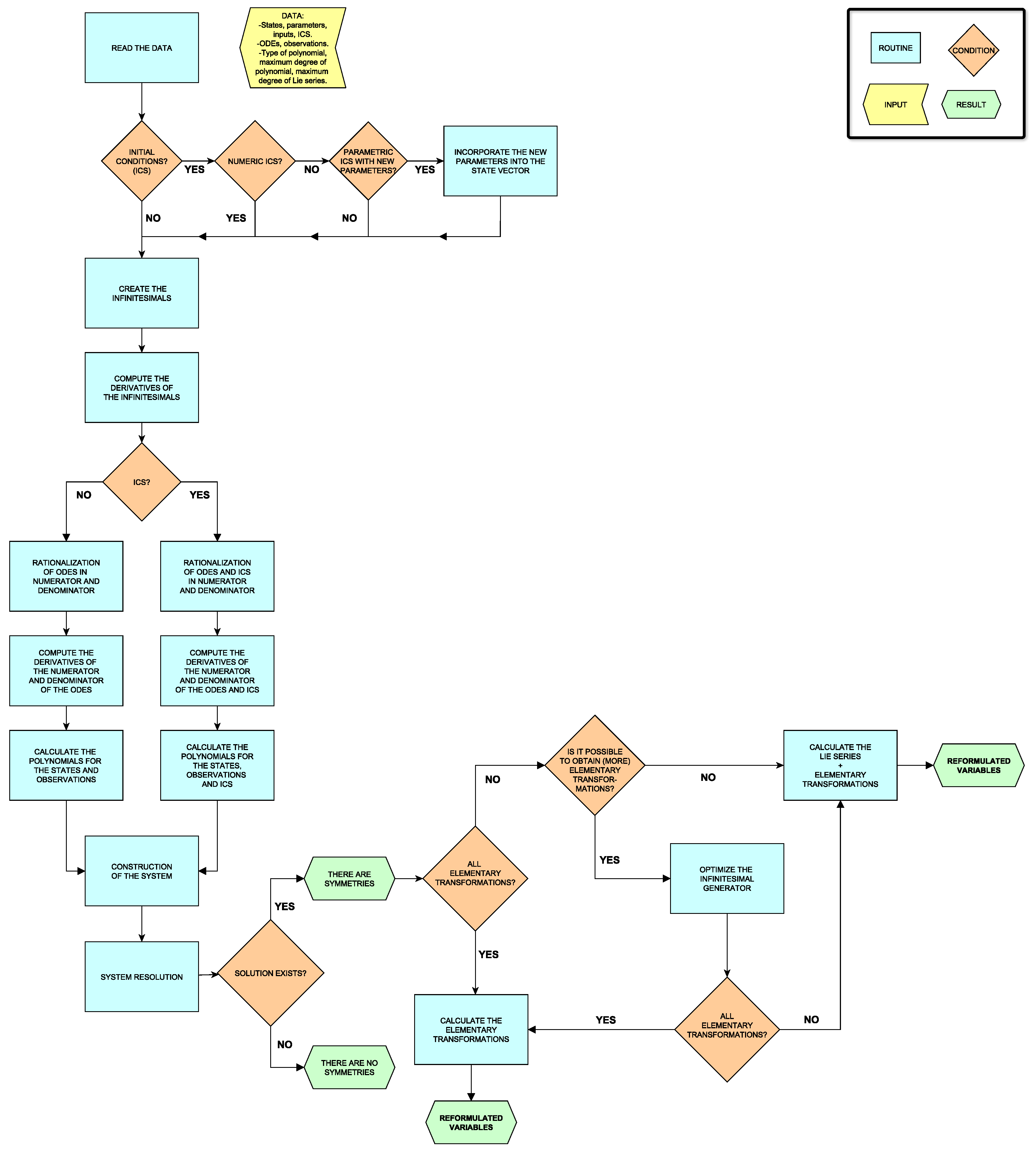
An overview of the algorithm described in the preceding subsections is shown in
Figure 1. We have made a MATLAB implementation available at
https://github.com/GemmaMasFes6/Lie-Symmetries, and as part of a new version (v2.1.6) of the STRIKE-GOLDD toolbox (
https://github.com/afvillaverde/strike-goldd_2.1); it will also be included in future releases of said toolbox. Our code represents an addition to the set of existing tools for studying differential equation symmetries, which include symmetryDetection [
15] in Python, MinimalOutputSets [
19] in Mathematica, and SADE [
21] in Maple. Our software is open source and, to the best of our knowledge, it is the first tool of its characteristics available in MATLAB.
The code consists of a main MATLAB script, ‘Lie_Symmetry’, and ten auxiliary functions defined in separate files. Each of these functions performs one of the stages outlined above: calculation of infinitesimal polynomials (univariate, partially variate and multivariate); computation of polynomials for states (depending on the type of polynomial there are two possibilities), observations, and ICS (if they are specified); and obtaining the transformations. The last step in turn incorporates two other functions, corresponding to maximizing the number of elementary transformations and, if necessary, calculating the transformations using Lie series.
The algorithm has a number of options that can be specified by the user: the type of infinitesimal polynomial, its degree, and the number of terms in Lie series (in case it has to be used).
The input of the programme must include the following vectors of symbolic variables, declared through the MATLAB sym command: parameters, states, initial conditions, ODEs, observations, and inputs (known or unknown). For initial conditions, two vectors must be provided: a vector called known_ics with entries equal to 1 for a known initial condition and 0 otherwise, and a vector ics with the values of the known ICS, either numeric or (known or unknown) parametric value.
The output of the programme first reports whether there is any symmetry. If a symmetry exists, the programme prints the infinitesimal generator and the transformations on the screen.
3. Results
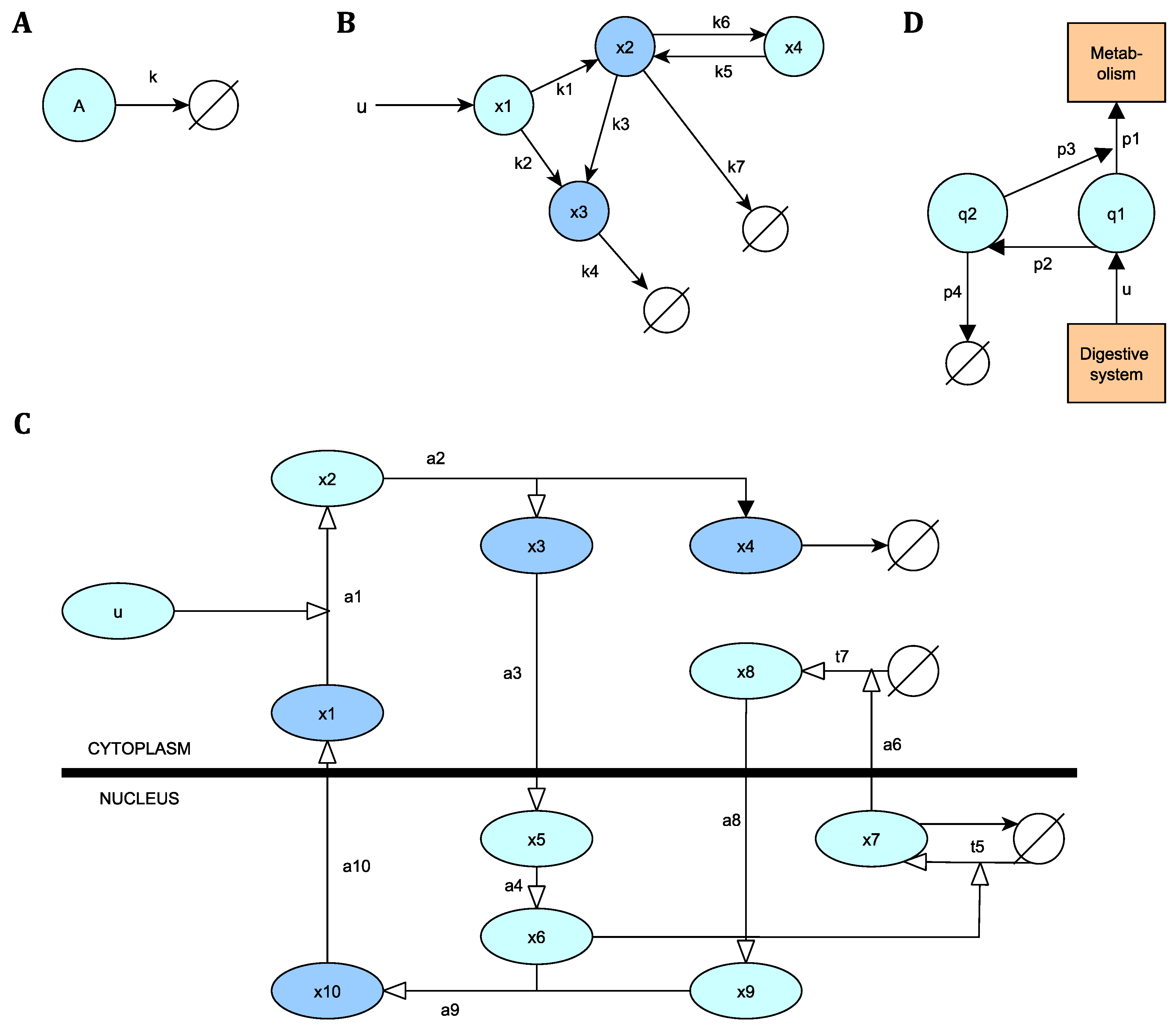
To illustrate the application of the method in biological and biomedical modelling, we use it to analyse a set of models taken from the literature. The models are listed in
Table 1 and their schematic representations are shown in
Figure 2.
3.1. Simple Chemical Reaction
This model represents a bimolecular reaction described by one ODE and one observation [
15]:
It is used to provide a basic illustration of the methodology, due to its simplicity. Without considering initial conditions, and using an univariate polynomial of second order, the programme finds two infinitesimal generators:
All the transformations are elementary:
Our results coincide with those reported in [
15]. It is possible to include ICS in order to study its influence in the model.
This example, because of its simplicity, allows us to check the results manually. Once the transformations are computed, it is easy to see that the second group of transformations solves the same ODE. The time derivative of
is:
Incorporating the above expression with
in (
33), the ODE is still fulfilled.
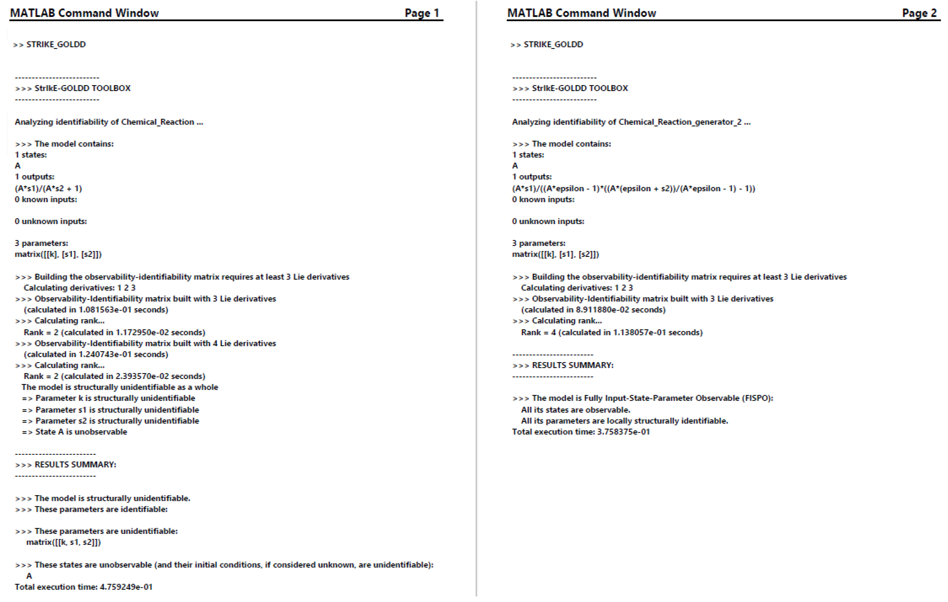
Below are two screenshots of the results of the observability and identifiability analysis obtained with STRIKE-GOLDD. In the first panel,
Figure 3 (Page 1), corresponding to the initial model, all states and parameters are unobservable; in the second one,
Figure 3 (Page 2), corresponding to the model with Lie transformations given by the second generator, states and parameters are observable.
3.2. Pharmacokinetic Model
A pharmacokinetic (PK) model describes the time course of the concentrations of a drug in different compartments, after entering an organism. This model includes one input, four ODEs, and two outputs [
22,
25]:
We use partial variate polynomials of second order, without ICS. Maximizing the number of elementary transformations leads to four of them, and the procedure yields the following infinitesimal generator:
The formulation of the IVP (
16) for this infinitesimal generator, considering only the non-elementary transformations, is:
| , |
| |
| , |
| |
| , |
| |
| , |
| |
| . |
The solution of the ODE system, replacing
with its transformation, is:
These new transformations coincide with those presented in [
25]. Using Lie series in the infinitesimal generator, the new expressions are:
These expressions seem to differ from the closed form, however, the result can be reformulated in order to obtain them. Taking as example
:
The last part of the previous expression consists of the first terms of the following series:
Substituting (
48) in (
47), the transformation of
is the same as the one obtained from IVP:
The most complicated case appears to be
. The expression obtained from the IVP (40) can be rearranged as:
It is only necessary to prove that (46) is the same as (
49) to show that both transformations are equal. Equation (46) can be reordered in terms of the powers of
:
The coefficient of
is
, as was proven before in (
47) and (
48).
The coefficient of the third term must be equal to
Considering the Taylor series of the previous expression until the fifth order,
we obtain that the final expression is the same as that presented in (
50).
The coefficient of
is the result of considering some terms of the Taylor series of
:
It is necessary to consider more terms of the Lie series to prove that the coefficient of
is
. In any case, regardless of the model under consideration, the transformations obtained with Lie series—that is, the output of the programme—are the expanding form of the solution of the IVP. In order to obtain a good approximation of the closed form (
36)–(40) the programme needs to consider sufficient terms of the Lie series. For this case, two terms are sufficient to achieve full observability (i.e., FISPO).
This model had been previously analysed in [
15,
25]. In [
15] a different infinitesimal generator was obtained; due to the lack of a method to compute non-elementary transformations, it was not possible to obtain all transformations. In [
25] the same infinitesimal generator as reported here was obtained, and transformations were computed using Hermite-Padé polynomials. The resulting transformations in [
25] are the same as those obtained from the IVP, as well as those obtained by our programme using Lie series.
3.3. NF-B Signalling Pathway
The model studied in this example was described in [
23,
26]. It represents a cellular signaling pathway found in most animal cells, corresponding to the NF-
B transcription factor. It is depicted in
Figure 2C, where black arrows indicate exit routes.
This model is the only one studied with ICS. In this case, they are parametric and include an additional parameter,
, that does not appear in the model equations:
Using a second order univariate polynomial, the following infinitesimal transformations were found:
Scaling symmetry was found for the known input function and two parameters:
The second symmetry was also for the input function and one parameter, in this case, a Mobius and translation symmetry, respectively:
Another scaling symmetry involving one state and two parameters:
One scaling type symmetry is admitted using the parameter
. All the nucleus states, as well as four parameters, take part in the symmetry:
The last symmetry is the only one that involves the initial condition parameter,
. All of the states have a scaling type symmetry, compensated by the scaling factor of
and
:
All of the symmetries are elementary transformations and it was not necessary to use Lie series. If ICS had not been considered, the symmetries would be elementary too.
This model was studied in [
15]. The results of the first four transformations presented above coincide with those found in [
15]; however, the last transformation includes the ICS parameter, unlike in the aforementioned article.
3.4. Glucose-Insulin Regulation
This model describes the regulation of blood glucose and insulin [
24]. It has two states (glucose and insulin), one output (a glucose measurement), and a known input (the glucose entering from the digestive system):
Here we analyse its symmetries without considering ICS. The model has two infinitesimal generators, which can be found using multivariate polynomials of second order:
The first infinitesimal generator includes only elementary transformations:
The second infinitesimal generator has seven transformations, four of which are elementary:
Considering two terms of Lie series, the reparameterized model is FISPO, as classified by STRIKE-GOLDD.
The formulation of the IVP for the second infinitesimal generator is:
| , |
| |
| , |
| |
| , |
| |
| , |
| |
| , |
| |
| . |
| . |
The solution of the ODE system is:
It is possible, using the procedure described for the pharmacokinetic model, to verify that the IVP solutions are the closed form of the solutions obtained through Lie series provided by the programme.
This model was proposed by Bolie [
24] and its structural identifiability was analysed in [
27] for the first time. However, its symmetries had not been studied until now.
4. Discussion
This article has addressed the relationship between non-observability and Lie algebra. Its main contribution is a computational method that searches for infinitesimal transformations in models composed of rational functions, in order to undo the symmetries that these may present. The procedure is based on expressing each transformation admitted by the ODE system according to its infinitesimal generator in polynomial form. In this way, the search for symmetries is equivalent to solving a system of linear equations, whose solution yields a transformation of the parameters that makes the model observable while leaving the observations invariant.
Our method builds on previous work [
12,
19,
25], and especially on the procedure presented by Merkt et al. [
15], with the addition of two features. The first one is the a priori maximization of the number of explicit transformations that can be obtained from the infinitesimal generator. The second one is the calculation of non-elementary transformations by means of Lie series. Increasing the number of explicit transformations is beneficial not only because it reduces the number of terms to consider from the Lie series, but also for calculating the solutions of the IVP. The complexity of the IVP solutions is inversely proportional to the number of explicit transformations. The pharmacokinetic model (PK) analysed here illustrates this point: without the use of the maximization of explicit transformations, MATLAB’s symbolic math toolbox did not manage to solve the IVP.
The algorithm allows to study the influence of the initial conditions in the model. The type of ICS (parametric, numeric or both) and the states that incorporate them may affect the number and type of symmetries of the models, varying from explicit to non-elementary transformations and reducing the number of infinitesimal generators.
We have implemented the method as a MATLAB programme that automates both the search for symmetries and the reconstruction of the model from the infinitesimal generators found. The programme has been integrated in the STRIKE-GOLDD toolbox for observability and identifiability analysis. The software has been tested with four previously published biomedical models, one of which—Bolie’s glucose-insulin regulation model—had not been tested for symmetries before. In the other cases our diagnoses mostly agree with those previously reported in the literature. An exception is the NF-
B model, for which we found an infinitesimal generator that includes the parameter introduced by the initial conditions and that was not found in a previous analysis [
15]. We observed another difference between our software and the one provided with [
15]: when analysing the chemical reaction (CR) and pharmacokinetic (PK) models, the generators obtained with our code remained the same when varying the type of polynomial and degree; in contrast, the generators obtained with the programme of [
15] changed when using partially varied and multivariate polynomials of order three or higher. These discrepancies may be due to implementation issues.
Our symmetry-detecting algorithm can be directly used to analyse structural identifiability and observability, providing an alternative to the OIC-checking algorithm already included in STRIKE-GOLDD for that purpose. More importantly however, this new code provides additional information about the relationships between model variables that cause loss of identifiability and/or observability. These insights can be exploited in two ways: (i) by fixing one or more parameters involved in a symmetry, in order to render the remaining ones identifiable, and (ii) by using the symmetry-breaking transformations to reformulate the model, yielding a modified model that is identifiable and observable. To facilitate the application of the latter procedure, we have implemented in our programme the semi-automatic transformation of a non-observable (respectively, non-identifiable) model into an observable (respectively, identifiable) model. It should be noted that, while said transformation may render a model fully observable, it also modifies the expression of the variables involved in its equations, which lose their original mechanistic meaning. Thus, while the results of the procedure can offer valuable insight about the model structure, they should be applied carefully for the purpose of model reformulation.
Our programme has some known limitations. First, while it considers high order generators and it can uncover a wide range of possible symmetries, it lacks procedures for determining a priori the type and total number of symmetries present in a model. Second, it does not provide a bound on the number of terms of the Lie series needed to obtain the infinitesimal transformations, when these are not given by explicit transformations. To the best of our knowledge, these limitations are shared with other existing methodologies. The possibility of overcoming them will be considered in future work.


