Analysis of Structural Changes in Financial Datasets Using the Breakpoint Test and the Markov Switching Model

Abstract

The price movements of commodities are determined by changes in the expectations about future economic variables. Crude oil price is non-stationary, highly volatile, and unstructured in nature, which makes it very difficult to predict over short-to-medium time horizons. Some analysts have indicated that the difficulty in forecasting the crude oil price is due to the fact that economic models cannot consistently show evidence of a strong connection between commodities and economic fundamentals, and, as a result, regarded the idea that economic fundamentals help predict price values as random luck. This study aimed to overcome the limitations of the economic models through the detection of structural changes as well as breaks in the data, using a breakpoint test. The Markov switching model is used to address the price patterns that led to a different market state. The results show that there are several changes as well as breaks in the estimated model. Moreover, there is an asymmetric correlation between the crude oil price and the GDP.

1. Introduction

Since the year 1980, the non-stationarity of financial data series has increasingly been taken into consideration. The non-stationarity of time series might be affected by time series components, such as the stochastic trend, the cyclical variation, or the seasonal variation. The non-stationary properties of financial data cannot simply be calculated through the application of filters in order to continue within the framework of stationary models [1,2]. A Markov switching model has been developed and thoroughly discussed [3,4]. However, it is analytically intractable. As a consequence, the conditions for covariance stationarity were not established. A multivariate Markov switching model that is analytically tractable was subsequently proposed [5]. The model also allows us to derive the stationarity conditions and further dynamic properties of the financial data. In the Markov switching model, all parameters allow us to shift between a high-volatility and a low-volatility regime. Moreover, different parameters for different regimes are allowed and defined as a regime-dependent volatility. A study revealed that the Markov model provides more reliability and availability in dealing with the problem, especially when the parameters can either fail or be repaired instantly [6].

The generalization of two Markov regression switching models is as follows:

$$\begin{array}{l}{Y}_t=X_1{B}_1+U_1\mathrm{for}\mathrm{regime}1\\ Y_t=X_2{B}_2+U_2\mathrm{for}\mathrm{regime}2\end{array}$$

(1)

where U₁ and U₂ are the random errors with normally distributed $\left(0,{\sigma }_1^2\right)$ and $\left(0,{\sigma }_2^2\right)$, and B₁ and B₂ are the coefficients of vector regression with the assumption that $\left({{\rm B}}_1,{\sigma }_1^2\right)\ne \left({{\rm B}}_2,{\sigma }_2^2\right)$. The probabilities λ and 1 − λ are a random or natural selection for regimes 1 and 2, where the probability λ is an independent state of the system.

There are numerous studies that examine the effect of oil price on the economy through different channels and methodology frameworks. The effects of oil price shocks and of the exchange rate volatility on inflation in Malaysia were studied, using data from January 2005 to November 2011, by adopting the Granger Causality Model [5]. The findings suggest that inflation does not granger cause the exchange rate, but granger causes the oil price. Likewise, the oil price granger causes inflation but does not granger cause the exchange rate. This shows that the oil price has a significant impact on inflation. In addition, a study was conducted to investigate the impact of oil price shocks on the output, inflation, and real exchange rate by drawing evidence from selected Association of Southeast Asian Nations (ASEAN) countries [7]. The results showed that the oil price fluctuations only had short-run effects on the countries. It was concluded that oil price shock does not induce much of the fluctuations in the ASEAN-5 economies. Another study [8] examined the price of ethanol and commodities in Brazil using the Bai–Perron test, the Johansen test, and the vector error correction model. The results showed that there was a short-term relationship between ethanol and commodities. However, to date, the nature of the relationship remains inconclusive, based on the past studies [9,10,11,12]. The volatility or the structural change is the common characteristic of the crude oil price. Crude oil prices are noisy, non stationary, non-linear, and unstructured in nature, which makes them very difficult to examine [13]. In order to evaluate the structural change of the time series, the Quandt–Andrews breakpoint test and the Bai–Perron test were used in this study to detect one or more unknown structural changes in the data. The Quandt–Andrews breakpoint test is derived from the Chow breakpoint test, to allow for a single Chow breakpoint test to be performed at every observation between two observations, and then summarized into one-test statistics.

This study had three aims: Firstly, it aimed to identify the structural changes in the crude oil price and the GDP using breakpoint tests. Secondly, the variables were tested using a co-integration test to investigate the short-run or long-run relationships. Thirdly, this study utilized the Markov switching regression to examine the effects of changes in the crude oil price on the GDP.

The remaining part of this article is presented in several sections: Section 2 discusses the theoretical aspect of the Markov switching model, Section 3 presents the data and the method, Section 4 shows the most relevant results and the discussion, and, finally, Section 5 summarizes the findings and provides the conclusions of our study.

2. Markov Switching Model

Linear regression is a popular statistical tool for econometric and statistical analyses. However, the nonlinearity of the time series might sometime cause less-precise and low-accuracy findings. A simple regression analysis is employed to explain the impact of changes in independent variables on a dependent variable.

A regression switching idea that uses a square root for each equation to represent the subsample was first introduced in 1958 [14]. The idea was then extended [15], by proposing a λ probability to avoid wasting information. The probabilities λ and 1 − λ were used in a two-state function $g\left(Y_j|X_j\right)$ [15], and the function is shown below:

$$\begin{array}{l}h\left(Y_j|X_j\right)=\lambda \left[g_1\left(Y_j|X_j\right)\right]+\left(1-\lambda \right)\left[g_2\left(Y_j|X_j\right)\right]\\ =\frac{\lambda }{\sqrt{2\pi }{\sigma }_1}\exp \left[-\frac{{\left(Y_j-X_j{\beta }_1\right)}^2}{2{{\sigma }_1}^2}\right]+\frac{1-\lambda }{\sqrt{2\pi }{\sigma }_1}\exp \left[-\frac{{\left(Y_j-X_j{\beta }_2\right)}^2}{2{{\sigma }_2}^2}\right]\end{array}$$

(2)

where j = 1, 2 …, M. The natural logarithm is used to maximize Equation (2) to obtain the values of the parameters in the model $\left({\beta }_1, {\beta }_2, {\sigma }_1^2,{\sigma }_1^2 \mathrm{and} \lambda \right)$ by using the equation (j = 1, …, M) below:

$$L={\displaystyle \sum _{j=1}^M\mathrm{In}h\left(Y_j|X_j\right)}$$

(3)

The Quandt model was then reviewed and enhanced [16], and it incorporated the Markov chain properties. A study revealed that the state changes in the variable series cannot be observed directly [16]. Each state in the estimated model is independent from each other, and the probability of a state is constant. The likelihood function in the Markov switching regression equation was corrected by suggesting a recursive algorithm to replace the likelihood function [17]. An algorithm was used to develop a filtering algorithm to calculate the conditional densities and the probability of the unobserved state value, $S_t$ [3,17].

$$Y_{t-1},P\left(s_t=j,s_{t-1}=i|Y_{t-1}\right)\mathrm{when}i,j=1,\dots ,M$$

(4)

This model has been further investigated and extended in two studies [4,18]. One study introduced a smoothing algorithm for the unobserved state variable [18], and the other extended it to the multivariate Markov switching model [4]. Another study examined the performance of the linear and the Markov switching model on the analysis of the stock price and the commodity price [19]. The Markov switching model performed better than the linear model, because it was able to detect the asymptotic behavior, and identified the expected duration for each state of the estimated model. It has been found that the Markov switching model outperforms when forecasting value at risk and expected shortfall of assets’ return [20]. It has also been reported that the Markov switching generalized autoregressive conditional heteroskedasticity (GARGCH) model is able to provide a more appropriate result in forecasting the volatility index [21].

3. Methodology

3.1. Data and Variables

The sample data were obtained from the United States (U.S.) Department of Energy, from Quarter 1 (Q1) 2010 to Quarter 4 (Q4) 2018. The benchmark crude oil price serves as a pricing reference to the sellers and buyers. The West Texas Intermediate (WTI), the Brent blend, and Dubai crude oil are the three primary benchmarks for crude oil. The oil that is traded in the United States of America (USA) is priced using the WTI as a benchmark, while most of the oil traded outside of the USA and the Far East is priced using the Brent blend as a benchmark. Dubai, however, is the main benchmark for the oil exported from the Middle East to Asia. The WTI crude oil, which is extracted from the wells in the southern part of the USA, specifically Oklahoma and Texas, has a very high quality of crude oil, with an American Petroleum Institute gravity of 39.6° and 0.24% of sulfur. Given these qualities, the WTI is the benchmark for light or sweet crude oil. The Brent blend crude oil is combined from different fields located in the North Sea, and it has an API gravity of 38.3° and 0.37% of sulfur, making it a light or sweet crude oil as well, although slightly less so compared with the WTI crude oil. The quality characteristics of both the WTI and Brent blend crude oil are quite similar, with the only difference being that the WTI crude oil results in rather more gasoline and rather less heating oil than the Brent blend crude oil. Consequently, the WTI crude oil has a slight price advantage compared with the Brent blend. On the other hand, Dubai’s crude oil has an API gravity of 32°, and it has a high sulfur content of roughly 2%; hence, it is considered to be the benchmark for heavy or sour crude oil. The light or sweet crude oil is usually traded at a premium to heavy or sour crude oil (Dubai). We use the Brent blend crude oil price as a proxy for the oil price, quoted in U.S. dollars in this study.

To measure the financial development, we used the country’s domestic variable, the GDP. Among the major economies of Asia, Malaysia is the second largest liquefied natural gas exporter in the world. According to the BP Statistical Review of World Energy, in 2015, 693,000 barrels of oil were produced in Malaysia and the average output over the past five years was 654,000 a day. The shipments of crude petroleum, petroleum products, and liquefied natural gas accounted for approximately 14% of Malaysia’s total exportations in the first half of the year 2016. Energy is a key sector of Malaysia’s GDP. As Malaysia is an oil net exporter, a high crude oil price may benefit the country in the short term. However, it can also be a disadvantage, since the rising prices of oil will have an impact on the world’s growth, which could affect the world’s consumption and income. Therefore, the focus of this study was to investigate the structural changes in and correlations between the price of crude oil and the GDP in Malaysia, using the Quandt–Andrews and the Bai–Perron breakpoint tests. The Markov switching regression model was used to analyze the correlations between oil price and GDP.

The Brent blend crude oil price has been widely used in previous studies [7,22,23], and the GDP used in this study was GDP per capita (in current U.S. dollars). These proxies have been widely used in previous studies [24,25,26]. The descriptive values for skewness and kurtosis in

Table 1. Descriptive statistics for the parameters.

	Mean	Standard Deviation	Skewness	Kurtosis	Jarqua–Bera
LOGOP	4.32	0.37	−0.34	1.81	2.85
MYGDP	71,410.50	5296.73	−0.39	2.29	1.66

indicated that all of the parameters were not normal. These results are consistent with the findings of the Jarqua–Bera test, and the statistics are non-negative and far from zero. Thus, there might be a structural change as well as breaks in the datasets.

3.2. Breakpoint Test

3.2.1. Quandt–Andrews Breakpoint Test

To identify the possible structural breaks, the Quandt–Andrews breakpoint test was used to specify the null hypothesis of no break is occurring within 15% of the trimmed data. Trimming the sampling data is mainly used to ensure that the subsample is not close to the endpoint of the sample [2].

The test statistic for examining the null hypothesis of no break at time period T, T₀ ≤ T ≤ T₁ is as follows:

QLR = max [c(T₀), c(T₀₊₁), …, c(T_1-1), c(T₁)]

(5)

where T₀ and T₁ are usually the inner 70% of the sample that is excluded from the first 15% and the last 15% of the sample.

3.2.2. Bai–Perron Test

The Bai–Perron test calculates the sup F statistics on no structural change (p = 0) on the null hypothesis and p = r changes. Let $M$ be a conventional matrix, such that ${\left(M\lambda \right)}^{\prime }=\left({\lambda }_1^{\prime }-{\lambda }_2^{\prime },\dots ,{\lambda }_r^{\prime }-{\lambda }_{r+1}^{\prime }\right)$. Then

$$F_T\left({\beta }_1,\dots ,{\beta }_r;q\right)=\frac{1}{T}\left(\frac{T-\left(r+1\right)q-p}{rq}\right){\widehat{\lambda }}^{\prime }{\mathrm{M}}^{\prime }{\left({\mathrm{M}}^{\prime }\widehat{\mathrm{v}}\left(\widehat{\lambda }\right){\mathrm{M}}^{\prime }\right)}^{-1}\mathrm{M}\widehat{\lambda }$$

(6)

where r is a break, and $\widehat{v}\left(\widehat{\lambda }\right)$ estimates the covariance matrix of $\widehat{\lambda }$ robust to serial correlation and heteroskedasticity. It is a generalization of the sup F test following Andrews (1993) and others,

$$\sup F_T\left(r,q\right)=F_T\left({\widehat{\beta }}_1,\dots ,{\widehat{\beta }}_r,q\right)$$

(7)

where $\left({\widehat{\beta }}_1,\dots ,{\widehat{\beta }}_r\right)$ is the global sum of squared residuals under the chosen trimming. This is equivalent to maximizing the F test since the estimated break dates are consistent, even in the presence of a serial correlation.

The breakpoint F-test is:

$$F=\frac{\left[\tilde{u}\tilde{u}-\left(u_1{u}_1+u_2{u}_2\right)\right]/k}{\left(u_1{u}_1+u_2{u}_2\right)/\left(T-2k\right)}$$

(8)

where ${\tilde{u}}^{\prime }\tilde{u}$ is the residual of the restricted sum of squares, $u_j^{\prime }{u}_j$ is the sum of squared residuals from subsample j, k is the number of parameters, and T denotes the total number of observations.

3.3. Co-Integration Test

The Johansen maximum likelihood estimator is a co-integration test that is powerful for analyzing the existence of a co-integration in the series. This estimator is able to provide asymptotically efficient estimates of the co-integrating vectors and adjustment parameters. Therefore, the Johansen test was applied in this study to examine the existence of co-integrating vectors among the variables [2].

3.4. Markov Switching Regression Model

The time series for all of the variables in this study vary with dynamics that are state-dependent [27]. The coefficients of the parameters may be different for each state, since the state can be in low or high volatility, or recession or expansion. Moreover, the time of transition and the duration in a particular state are both random. Therefore, the Markov switching regression was used to estimate the state-dependent parameters. The framework for the Markov model is to be memoryless in each individual state [27]. Thus, the switching properties can be calculated by using the following equation:

$$MYGD{P}_t={\mu }_i+\alpha logO{P}_t+{\epsilon }_t$$

where ${\mu }_i$ = ${\mu }_1$ if i = 1 (state 1), and ${\mu }_i$ = ${\mu }_2$ if i = 2 (state 2). The transition probabilities for a two-state model are:

$$\left[\begin{array}{cc}{p}_{11}& p_{12}\\ p_{21}& p_{22}\end{array}\right]$$

where $p_{11}+p_{12}=1, p_{21}+p_{22}=1$. The expected duration for each state is important to identifying the asymmetric properties for the business cycle. The expected duration can be estimated by using the following formula: $E\left(D\right)=\frac{1}{1-p_{ii}}$, where i is the state/regime.

4. Results and Discussions

The results of the analysis are shown and discussed below.

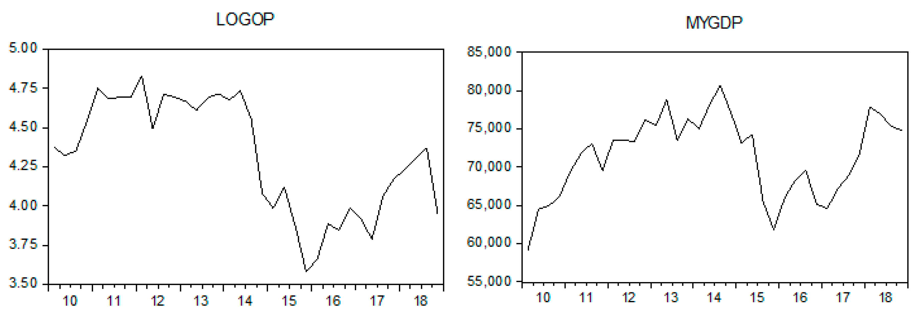
Figure 1 shows the changes in the data series. All of the variables that are plotted in Figure 1 are irregular, suggesting that the variables series are not stationary. Additionally, there are several structural changes present in the series, including the 2011 quarter 2, the 2012 quarters 1 and 2, the 2015 quarters 1, 3, and 4, the 2017 quarter 2, and the 2018 quarter 3. All these changes can be related to an economic crisis such as the Global Economic Crisis of 2012, witnessing the European debt crisis, with a dramatic depression in 2011, the Chinese stock market crash, the Russian financial crisis of 2014–2017, etc. Malaysia is an emerging market that is undergoing rapid growth, and is keen to be affected by other countries, especially trading partners, as mentioned in [28]. Therefore, we can conclude that these series have regime shifts due to the uncertainty in the parameters’ series.

The p-value for the Quandt–Andrews breakpoint test in

Table 2. Findings of the Quandt–Andrews breakpoint test.

Quandt–Andrews Unknown Breakpoint Test
Null Hypothesis: No Breakpoints within 15% Trimmed Data
Varying Regressors: All Equation Variables
Statistic	Value		Prob.
Maximum LR F-statistic (2012Q2)	21.39673		0.0000
Maximum Wald F-statistic (2012Q2)	42.79346		0.0000
Exp LR F-statistic	8.147680		0.0000
Exp Wald F-statistic	18.32268		0.0000
Ave LR F-statistic	9.538625		0.0001
Ave Wald F-statistic	19.07725		0.0001

Note: probabilities calculated using Hansen’s (1997) method. Prob.—Probability.

is at a less than 0.05 level of significance. Thus, we can conclude that there are breaks in the sample data. We next identified the break date by using the Bai–Perron test.

The estimated break dates suggested by the Bai–Perron tests in the

Table 3. The Bai–Perron test outputs.

Multiple Breakpoint Tests
Bai–Perron Tests of L+1 vs. L Sequentially Determined Breaks
Break Test Options: Trimming 0.15, Max. Breaks 5, Sig. Level 0.05
Sequential F-statistic determined breaks:			2
		Scaled	Critical
Break Test	F-statistic	F-statistic	Value **
0 vs. 1 *	21.39673	42.79346	11.47
1 vs. 2 *	7.279554	14.55911	12.95
2 vs. 3	4.667017	9.334033	14.03
Break dates:
	Sequential	Repartition
1	2012Q2	2012Q2
2	2015Q3	2015Q3

* Significant at the 0.05 level, ** Bai–Perron (Econometric Journal, 2003) critical values. Max.—Maximum; Sig.—Significance.

are Quarter 2, 2012 and Quarter 3, 2015. This might be related to the great recession in the United States, and the 2015 Chinese stock market crash. China was the largest trading partner of Malaysia between 2009 and 2017 (16.4 per cent or 67,229 million U.S. dollars (USD); and the United States was Malaysia’s third largest trading partner in 2017, which contributed 8.9 percent or 36,623 million USD. Unstable economic conditions in these two countries can affect the GDP in Malaysia.

To understand the co-integration impact of the time series variables, the Johansen co-integration test was used to evaluate the variables series. The findings are presented as follows.

Table 4. The co-integration test outputs.

Unrestricted Co-Integration Rank Test (Trace)
Hypothesized		Trace	0.05
No. of CE(s)	Eigenvalue	Statistic	Critical Value	Prob.**
None	0.226176	12.01652	20.26184	0.4473
At most 1	0.092458	3.298539	9.164546	0.5264
Hypothesized		Max. Eigenvalue	0.05
No. of CE(s)	Eigenvalue	Statistic	Critical Value	Prob.**
None	0.226176	8.717976	15.89210	0.4647
At most 1	0.092458	3.298539	9.164546	0.5264

Trace test indicates no co-integration at the 0.05 level, * denotes rejection of the hypothesis at the 0.05 level, ** MacKinnon–Haug–Michelis (1999) p-values, Unrestricted Co-integration Rank Test (Maximum Eigenvalue), Max. eigenvalue test indicates no co-integration at the 0.05 level.

shows that all the p-values are greater than 0.05. There is no co-integration between Malaysia’s GDP and the oil price. There is a short term relationship between the changes in oil price and the GDP. This finding is consistent with previous results [7], indicating that the oil price fluctuations only have short-run effects on the inflation, real exchange rate, and GDP in Malaysia.

Table 5. The Markov switching regression outputs.

Method: Markov Switching Regression (BFGS/Marquardt Steps)
Number of states: 2
Initial probabilities obtained from ergodic solution
Ordinary standard errors and covariance using a numeric Hessian
Random search: 25 starting values with 10 iterations using 1 standard
deviation (rng = kn, seed = 1,560,858,386)
Convergence achieved after 28 iterations
Variable	Coefficient	Std. Error	z-Statistic	Prob.
Regime 1
LOGOP	10,254.71	1877.429	5.462102	0.0000
C	29,104.07	7933.635	3.668440	0.0002
Regime 2
LOGOP	21,525.61	6420.504	3.352635	0.0008
C	−30,461.34	29431.43	−1.034993	0.3007

Std.—Standard.

reported the outputs for Markov switching regression. Two regimes of the Markov switching models were selected in this study as suggested by previous studies [29,30] indicating that two-regime models can represent the recession and growth states in the business cycle. A Marquardt step is used in the Markov switching regression model to estimate the parameters of an unobserved state. The findings show that there is a positive correlation between the oil price and the GDP. These results are consistent with previous findings [31], but contradict others [32,33]. It has been argued that the negative effect of oil price shocks on GDP growth is greater than the time of oil price increases [32]. In addition, a study has revealed that the relationship between the GDP and the oil price is relatively turbulent [32]. The changes in the relationship rely on the economic conditions, such as the stability, recession, and growth conditions. Previous studies [32,33] agree that the correlations between the oil price and the GDP are unstable and vary in different phases over time. The present study is expected to provide better insights into the relationship between the oil price and the GDP, since we have divided the datasets into two regimes (regime 1: growth, and regime 2: recession) while measuring the relationship between the oil price and the GDP.

The transition probabilities in the

Table 6. The transition probabilities and expected durations.

Constant Markov Transition Probabilities
Sample: 2010Q1 2018Q4
Included observations: 36
P(i, k) = P(s(t) = k | s(t − 1) = i)
(row = i/column = j)
		1		2
All periods	1	0.975638		0.024362
	2	0.043480		0.956520
Expected duration: Constant Markov transition
probabilities
Sample: 2010Q1 2018Q4
Included observations: 36
Constant expected durations:
	1		2
All periods	41.04773		22.9920

reported from regime 1 to regime 2 are higher than the transition probabilities from regime 2 to regime 1. This indicates that the recovery variable needs a longer time than the stagnant variable. p₁₁ and p₂₂ have a high value; thus, we rejected the null hypothesis of no shifts in the regime.

Based on the findings of expected durations, we can conclude that there is an asymmetric business cycle, since the expected durations in regimes 1 and 2 are approximately 41.048 and 22.999 quarters, respectively. The first regime is more prevalent than the second regime. The results are consistent with previous findings [34,35,36], indicating that there is an asymmetric oil shock.

5. Conclusions

The crude oil price is non-stationary, highly volatile, and unstructured in nature, which makes it difficult to forecast over short-to-medium time horizons. Past studies [29,30,31,32,33,34,35,36] have also shown that the inconsistency may lie in the intrinsic limitations of the theoretical framework, or in ignoring the time series components. The present study aimed to overcome the limitations of the economic models through the detection of the structural changes in the data series, using the breakpoint test and the Markov switching regression model to address the price patterns that led to different market states. The results of the Quandt–Andrews test show the existence of breaks in the data. Moreover, the estimated break dates are Quarter 2, 2012 and Quarter 3, 2015. Based on the Markov switching regression outputs, the oil price has a positive relationship with the GDP, where the increase of the oil price impacts the increase of the GDP. However, according to the transition probabilities and the expected duration results, there is an asymmetric relationship between the oil price and Malaysia’s GDP. Even though Malaysia is an oil exporter, it is not a member of Organization of the petroleum exporting countries (OPEC). This indicates that Malaysia has no influence on the determination of the oil price internationally.

This study has some limitations that future research can address. One such limitation is that we used quarterly data, while daily or monthly data may provide a greater understanding of the breaks in or changes of the time series. Future research may also include daily or monthly data for a better understanding of the changes in the oil price. The results of this study can also be expanded to other financial or economic variables, such as the stock price and exchange rate, to expand the multivariate framework. Further studies with this method can be extended to a three-regime Markov switching model to measure three states: depression, high appreciation, and low appreciation, as suggested previously [37].