Article

Use of Precise Area Fraction Model for Fine Grid DEM Simulation of ICFB with Large Particles

1
School of Mathematics and Statistics, Chongqing Three Gorges University, Chongqing 46000, China
2
Department of Applied Mathematics, Northwestern Polytechnical University, Xi’an 710072, China
*
Author to whom correspondence should be addressed.
Symmetry 2020, 12(3), 399; https://doi.org/10.3390/sym12030399
Submission received: 8 January 2020 / Revised: 9 February 2020 / Accepted: 17 February 2020 / Published: 4 March 2020
(This article belongs to the Special Issue Fixed Point Theory and Computational Analysis with Applications)

Abstract

:
The heterogeneous structures in a gas–solid fluidized bed can be resolved in discrete element simulation so long as the grid is fine enough. In order to conveniently calculate mean porosity in fine grid simulations, a precise area fraction model is given for two-dimensional simulations. The proposed area fraction model is validated by the discrete element simulation test on a small-scale internal circulation fluidized system of large particles, using a fine grid size of two particle diameters. Simulations show that the discrete element method can perform well in modelling time-varying waveforms for the physical quantities in an internal circulating fluidized bed, employing the precise gas area fraction model. This thought of precise calculation can be generalized to construct a volume fraction porosity model for three-dimensional simulation by use of the similar symmetry of a rectangular grid. Moreover, to construct these area and volume fraction models is to enrich and perfect the underlying model of fine grid simulation.

1. Introduction

Internal circulating fluidized beds (ICFB) can find lots of applications in industrial fields such as energy, environment, chemical engineering, etc. [1]. The non-intrusive access of an ICFB is too difficult to hamper the detailed experimental study of granulation. As a complement to experimental study, numerical methods are being used more and more frequently for simulating gas–solid two-phase flow behaviors and transfer characteristics which are significant for the design of an ICFB. Among these methods, the discrete element method (DEM) [2,3,4,5] deals with the solid phase as discrete particles, and thus is advantageous in providing the particle level information. DEM has become a powerful tool in fluidized bed researches and has shown good prospects.
However, the reliable applications of DEM simulations for various fluidized operation types need to be further validated in many ways. Now DEM can find its mature applications in simulations of fundamental fluidization phenomena and analysis of qualitative tendencies, rather than in quantitative researches. Since parameters for both gas and solid phases are calculated within grid circumstance in DEM simulation, results have much to do with the grid size chosen. For example, if one uses a coarse grid in a common DEM simulation code, the distinct heterogeneous particle distribution within the grid will cause large deviation in the calculated drag force [6,7]. On the contrary, fine grid simulation, although it has high spatial resolution, will lead to the complexity of parameter calculation.
Nowadays more and more researchers tend to use a fine grid in their DEM simulations [8,9,10,11]. It can be easily imagined that a fine grid is advantageous in reducing the amount of smoothing of the flow field. It is suggested that the fine grid size of 2–4 particle diameters be sufficient to resolve the complex structures in fluidized beds of various types of particles [12]. Moreover, the main issue of computational limitation in DEM simulation is that it roots in large numbers of particles required, rather than the use of a fine grid. Thus it is both necessary and possible to use a fine grid in DEM simulations.
Unfortunately, the theoretical system of fine grid simulation is far from perfect. The complexity mainly lies in the proper calculation of grid porosity and local porosity, the simulation sensitivity to both of which is high. On the one hand, local porosity is the virtual parameter centered at a particle, which is in fact independent of the grid. It should be calculated accounting for the complex circumstances, often with a heterogeneous particle distribution. Since the existence of a surrounding particle can lead to a comparable deduction of local porosity, the calculation scale for local porosity should be larger than the fine grid scale. On the other hand, in two-dimensional simulation, grid porosity must be obtained from two-dimensional grid porosity, i.e., gas area fraction, which can be precisely calculated theoretically. However, the precise model has never been given in the literature.
This article mainly discusses the methodology of two-dimensional fine grid simulation despite the relative convenience of coarse grid simulation. In this research, the grid porosity and the local porosity are independently calculated. In our previous work [7], a local porosity model independent of grid is used to improve the method of drag calculation. In this work, a precise area fraction model is given to properly calculate the grid porosity. This model is validated by the DEM simulation test on a real small-scale ICFB of large particles, using grid size of two particle diameters.

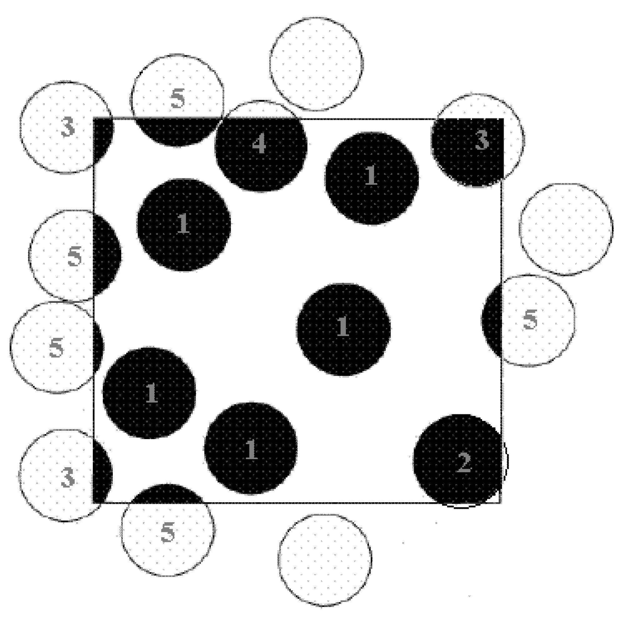
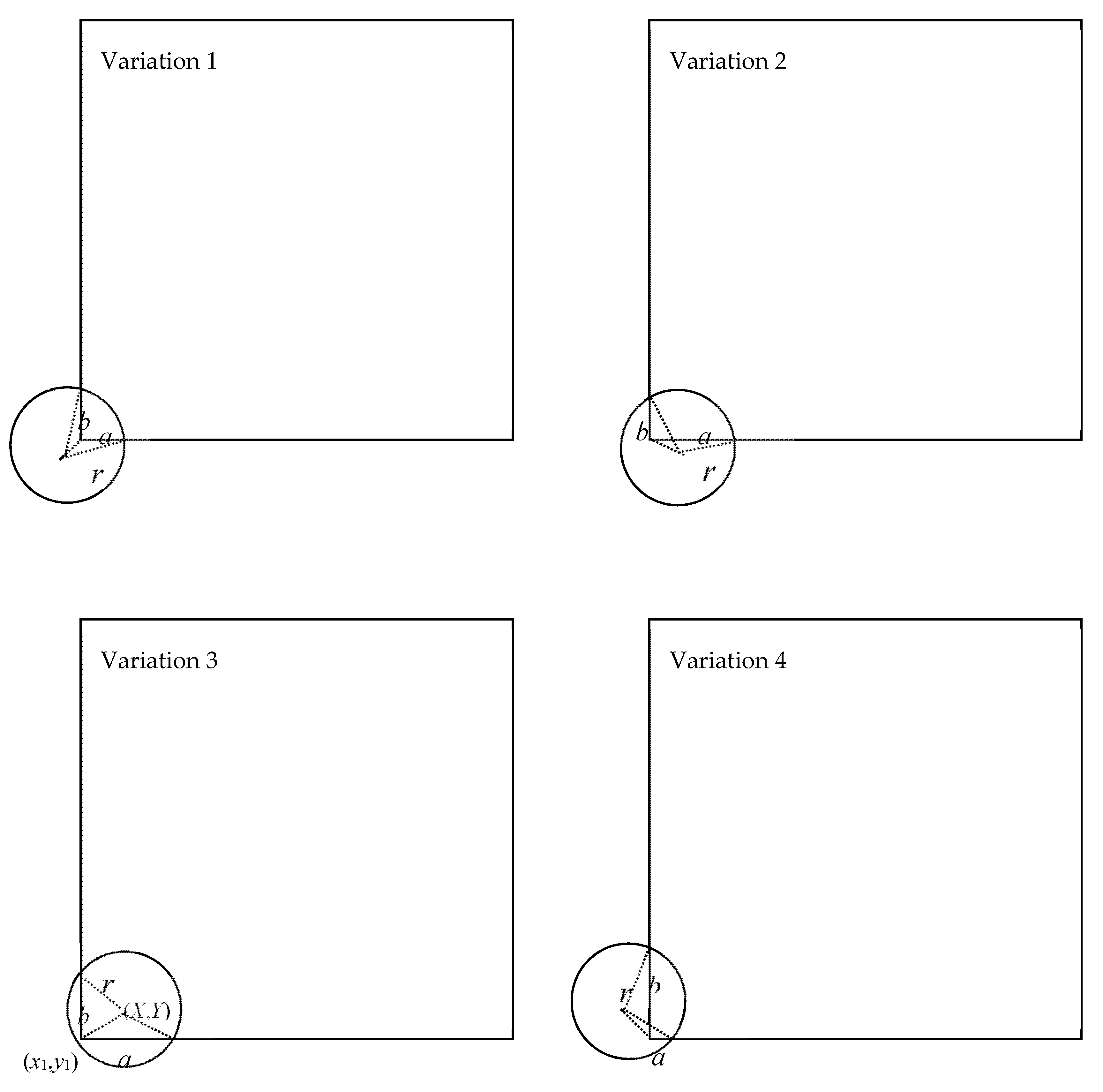
2. Precise Area Fraction Model

In general, two-dimensional grid porosity, i.e., the gas area fraction, can be expressed as
ε 2 D = 1 ε 2 p = 1 k = 1 N f i
where ε 2 p is the solid area fraction, f i is the grid area occupied by particle i and N is the total number of particles overlapped with the grid. For fine grid simulation, a detailed check of overlap should be made and thus the precise expression of f i is complicated. In the following, we will give a precise area fraction (PAF) model.
Figure 1 shows all five cases of particle-grid overlap. For convenience of editing a model code, the five cases when the particle center is relatively close to a certain grid vertex should be separately analyzed. Figure 2 shows the region divisions of the particle-grid overlap. If the particle center is in the total region noticed, then f i   > 0. The lower-left one fourth of the total region determined by the grid center ( x , y ) is also noticed. If the particle center is in this region, it is relatively close to the lower-left grid vertex. Moreover, the lower-left region is further divided into five sub-regions which correspond to the five cases of grid–particle overlap.
According to Figure 2, when the particle center is relatively close to the lower-left grid vertex, there are five cases of grid-particle overlap. Here it is assumed that a square grid is used, and the grid side is at least two times longer than the particle diameter. As will be seen, the model can be easily generalized to a rectangular grid because of similar symmetry. Figure 3 gives the first two cases. For Case 1, the particle center ( x , y ) satisfies x 1 r < X < x and y 1 r < Y < y . Then f i is calculated as
f i = 1 d x · d y π r 2
For Case 2, it satisfies that x 1 r < X < x , y 1 r < Y < y and ( X x 1 ) 2 + ( Y y 1 ) 2 < r . Then f i is calculated as
f i = 1 d x · d y [ π r 2 r 2 arccos X x 1 r r 2 arccos Y y 1 r + 1 2 r 2 sin ( 2 arccos X x 1 r ) + 1 2 r 2 sin ( 2 arccos Y y 1 r ) ]
Figure 4 shows Case 3 when the particle center is relatively close to the lower-left grid vertex. For this case, there are four variations for which the particle center satisfies ( X x 1 ) 2 + ( Y y 1 ) 2 < r . However, the expressions of f i for the four variations are formally consistent. According to Figure 4,
a = r 2 ( Y y 1 ) 2 + ( X x 1 )
b = r 2 ( X x 1 ) 2 + ( Y y 1 )
Then f i is calculated as
f i = 1 d x · d y [ 1 2 r 2 arccos 2 r 2 a 2 b 2 2 r 2 + 1 2 a ( Y y 1 ) + 1 2 b ( X x 1 ) ]
Figure 5 shows Case 4 when the particle center is relatively close to the lower-left grid vertex. For this case, there are two variations. For the first variation the particle center satisfies x 1 < X < x 1 + r and y 1 + r < Y < y . Then the expression of f i is
f i = 1 d x · d y [ π r 2 r 2 arccos Y y 1 r + 1 2 r 2 sin ( 2 arccos Y y 1 r ) ]
For the second variation the particle center satisfies x 1 + r < X < x ,   y 1 < Y < y 1 + r . Then the expression of f i is
f i = 1 d x · d y [ π r 2 r 2 arccos X x 1 r + 1 2 r 2 sin ( 2 arccos X x 1 r ) ]
Figure 6 shows Case 5 when the particle center is closer to the lower-left grid vertex. For this case, there are also two variations. For the first variation, the particle center satisfies x 1 < X < x ,   y 1 r < Y < y 1 . The expression of f i is
f i = 1 d x · d y [ r 2 arccos x 1 X r 1 2 r 2 sin ( 2 arccos x 1 X r ) ]
For the second variation, the particle satisfies x 1 r < X < x 1 ,   y 1 < Y < y . Then the expression of f i is
f i = 1 d x · d y [ r 2 arccos x 1 X r 1 2 r 2 sin ( 2 arccos x 1 X r ) ]
For the above five cases,   f i is calculated provided that the lower-left grid vertex is relatively close to the considered particle. If the considered particle is relatively close to another grid vertex, f i can be similarly calculated. Put f i into Equation (1) and calculate the precise ε 2 p and ε 2 D , then we construct the PAF model.

3. Extension to Three-Dimensional Simulation

We have constructed a three-dimensional porosity model which considers all the cases of particle-grid overlap. Let us take just a particle to be a sphere and a grid to be a cube. Figure 7 gives the schematic of all nine cases of particle-grid overlap. For Case 2 to Case 4, the solid volume can be obtained by precisely calculating the volume of the sphere minus the volume of one, two or three spherical segments, respectively. However, generally the solid volume is complicated and cannot be precisely calculated for the rest of the five cases.
The intersected geometries in Case 5 and 9 are called quasi semi-segment and quasi quarter-segment, respectively. Then the intersected solid volume for all cases can be uniformly expressed as
V solid = V k sphere V l segment ( s ) + V m quasi semi segment ( s ) + V n quasi quater segment
where k and n are equal to 0 or 1, l and m are equal to 0, 1, 2 or 3. As is known, Vsphere and Vsegment can be easily and precisely calculated. In fact, one can also directly calculate Vquasi semi-segment and Vquasi quarter-segment by use of a single mathematical formula, employing the double definite integral and compound numerical integral. See [13] for more details.

4. Simulation Methods

Gas motion over grid k is determined by the Navier-Stokes equations as
( ε g ρ g ) t + · ( ε g ρ g u ) = 0
( ε g ρ g u ) t + · ( ε g ρ g u u ) = ε g p · ( ε g τ g ) + ε g ρ g g β ( u i = 1 N k v i N k )
where ρ g is the gas density, u is the gas velocity, p is the gas pressure, v i is the velocity of particle i , τ g is the viscous stress tensor, β is the momentum exchange coefficient [14], and N k is the number of particles within the grid.
The last term in Equation (13) is the coupling term. This way of coupling, although less frequently adopted by researchers, seems to be more capable of predicting bed expansion [7,15]. Xu and Yu [4] argued that the coupling between gas-solid two phases should follow Newton’s third law of motion. That is to say, drag force on individual particles should react on gas from individual particles. Although the strictly coupling ways is widely used, according to Feng and Yu [16], the difference between the simulations is less significant unless a large particle layer keeps fluidized in the flow region close to the inlet. As the gas–solid interaction scale is thought to be larger than the fine grid scale, we forgo the use of the frequently-adopted coupling way.
The gas area fraction ε 2 D of a grid is calculated by the proposed PAF model. Note that drag correlation is based on the real three-dimensional experimental results. The grid porosity in the Navier–Stokes equations should be three-dimensional porosity ε 3 D which is ε g in Equations (13) and (14). Then ε 2 D is transformed into ε 3 D [4] as
ε 3 D = 1 2 π 3 ( 1 ε 2 D ) 3 2 .
Equations (12) and (13) are discretized by the finite volume method based on the collocated grid. Uniform velocity inlet, pressure outlet and impermeable wall are defined as the boundary conditions. The Navier–Stokes equations are solved according to the method in [17].
The soft-sphere model is used to deal with particle-particle and particle-wall collisions. Presently the time step for the gas motion is 0.00005 s and the DEM time step is 0.00001 s. This DEM time step is much smaller than the required maximum time resolution [2] defined by the spring constant.
The translational motion of each particle i is determined by
ρ p V p d v i d t = ρ p V p g + F D i + F C i V p p i
where ρ p is particle density, V p is particle volume, F D i is drag force, F C i is collision force and p i is local gas pressure.
The rotational motion of particle i is described as
I d ω i d t = T C i
where ω i is the particle angular velocity, I is the inertia moment of the particle as spherical and T C i is the torque due to collision.
The drag force F D i is computed by the Wen and Yu correlation [14], using a so-called complete circumstance-independent model to calculate local porosity [7], as
F D i = 1 8 π d p C D i ρ g | u i v i | ( u i v i ) ε i 2.7
where u i is the local gas velocity which is calculated by area weighted averaging, and the standard drag coefficient C D i is expressed as
C D i = { 24 ( 1 + 0.15 Re i 0.687 ) Re i , Re i 1000 , 0.44 , Re i > 1000 .
The Reynolds number of particle i in Equation (18) is
Re i = ε i ρ g | u i v i | d p μ g .
In the present simulations, the parameters involved are given in Table 1, with the geometry, operation conditions and material properties basically similar to those in the experimental research of van Wachem et al. [18].

5. Results and Discussion
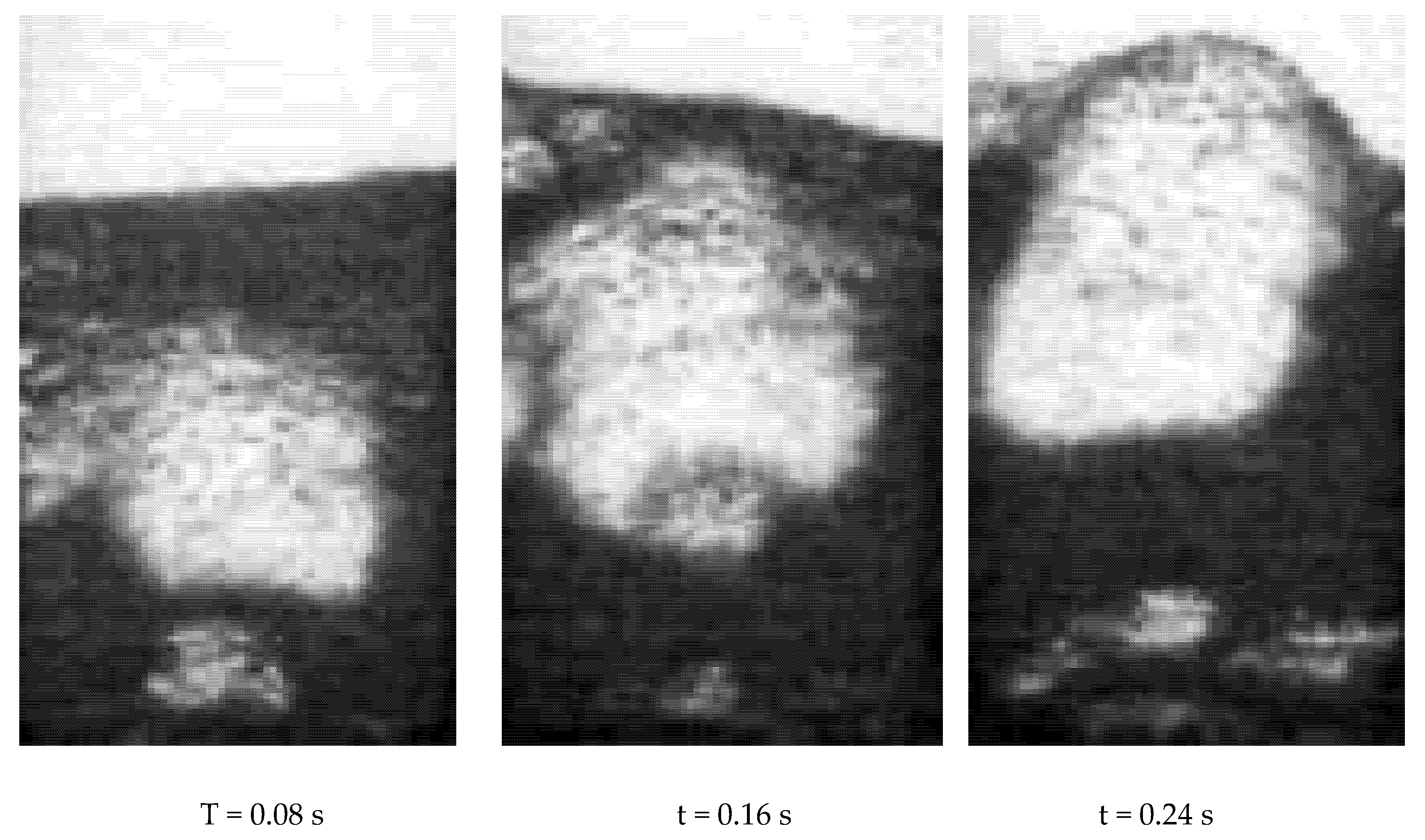
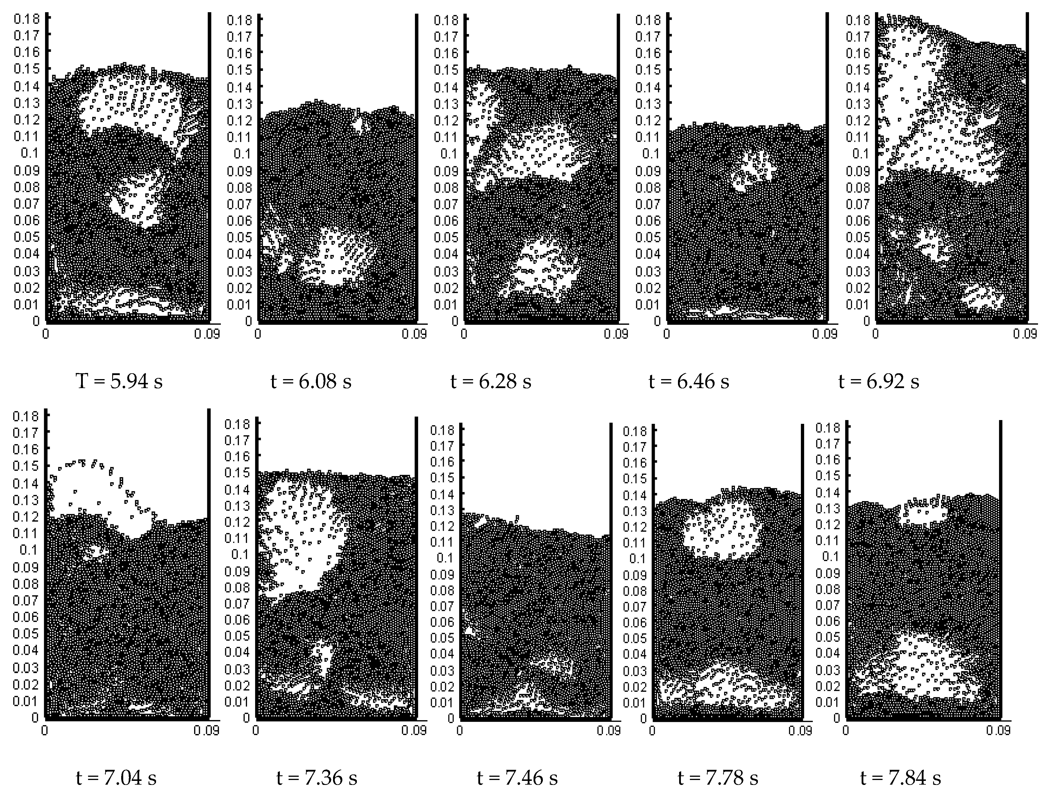
5.1. Big Bubble

Figure 8 demonstrates the particle distributions in the present simulations and previous experiments [18]. The simulated bubble size is in agreement with that in the experiments. The inconsistency of bubble shape may indicate that the real complicated inlet effect cannot be properly reflected by just setting the simple inlet boundary condition. In the simulations the bubble wake effect is stronger than in the experiments. Thus at 0.42 s, the bubble seems bullet-bottom; while at 0.5 s, there are much more particles thrown into the big bubble.

5.2. Solid Volume Fraction

It has been reported that traditional coarse grid DEM simulations may capture some features which deviate from experiments [18]. Drag calculation was improved and better simulations were obtained in our coarse grid simulation work [6,7]. Those previous simulation results should be referred to, but are not given in the following. Only the present simulation results and the pertinent experimental results are given for comparison to validate the present fine grid simulations.
Figure 9 demonstrates the measured and calculated solid volume fraction fluctuations which are averaged in the horizontal plane at 45 mm above the distributor. Although small amplitude fluctuations can be seen in both the experiments and the present simulations, there are more of them in the simulations. Thus, the simulated fluctuations seem a little faster than the measured. The former traverse about 9 cycles in 5–7 s while the latter traverse about 7.5 cycles in 2–4 s. The simulated solid volume fraction fluctuation slightly deviates from the waveform shown in the experiments. This deviation may partly result from the calculation method for the solid volume fraction in the simulations. The solid volume fraction is computed as one plus ε 3 D . However, the transformation of ε 2 D to ε 3 D is adopted, which to some extend may deviate from the real value of porosity, although this transformation formula is widely used. On the whole, the simulated waveform for the solid volume fraction is as good as that in [7], which is much more consistent with the experiment data than that in [6,18].

5.3. Relative Pressure

Figure 10 demonstrates the measured and presently-calculated relative pressure fluctuations which are averaged in the horizontal plane at 45 mm above the distributor. Both the simulated and measured relative pressure values are between –200–200 Pa. As is noticed, small amplitude fluctuations of relative pressure occur in both the experiments (from 3 to 3.75 s) and the present simulations (from 5.5 to 6.25 s). This reflects the random and instable features of the real fluidization. The unconformity of the two frames in the figure lies in the waveforms. The simulated waveform reveals weaker periodicity. Pressure is a basic variable of the Navier–Stokes equations. It is hard to be accurately calculated, which mainly lies not in calculation error, but in model error. The momentum exchange source term in Equation (13) represents the gas-particle interaction which is calculated by the widely used correlation formula proposed by Wen and Yu [14]. This model error may be reduced in two ways. One way is to develop structure-dependent drag force in a coarse grid simulation [6]. Another way is to use a fine grid so that the heterogeneous structure can be fully resolved, which is also adopted in this work. Without consideration of the small amplitude fluctuations during the similar period of 0.75 s, the calculated fluctuations traverse about 6.5 cycles while the measured fluctuations traverse about 5.5 cycles. In this sense, the simulated fluctuation frequency is better than that in [7].

5.4. Bed Layer Height

Since in the study conducted by van Wachem et al. [18], the expression of bed layer height H was not given, we use a visual observation technique as in [7], rather than the on-line output technique as in [6]. Figure 11 shows the simulated particle locations at the time nodes of the locally highest and lowest bed layer height. Figure 12 shows the measured and presently-simulated bed layer height expansion. Again, it is noticed that the waveforms are the most distinct difference. The simulated time-varying H seems like a piecewise linear function of time because it is approximated by just using local extremes. In [7], both the mean minimum and maximum values of the simulated H are a little higher than those in the experiments. However, in the present simulations, both the mean minimum and maximum values of the simulated H are very close to those in the experiment. The simulated fluctuations traverse about five cycles in 6–8 s while the measured fluctuations traverse about 5.5 cycles in 2–4 s. The simulated fluctuation frequency is only a little lower than the measured fluctuation frequency. These results show that the bed expansion in the present simulations is better than that in the previous simulations [7]. Moreover, the tendency of slow expansion and fast fallback, shown in the experiments, can be well described in the present simulations.

6. Conclusions

This article suggests that the use of a fine grid is beneficial to resolve the complex heterogeneous structures in fluidized beds of various types of particles. The major complexity of fine grid simulation is thought to lie in the calculation of grid parameter. The article mainly presents a porosity model and validates it in two-dimensional simulation of an ICFB. The following conclusions can be obtained.
(1)
The PAF model is given to precisely calculate the solid or gas area fraction, and theoretically to more properly calculate the grid porosity.
(2)
The simulated big bubble is generally consistent with the experiment results in shape and size. The present simulation works well enough to model the basic bubbling phenomenon of an ICFB.
(3)
The simulated fluctuation time scales and amplitudes of solid volume fraction, relative pressure and bed layer height are close to the experimental results, showing that DEM can perform well in modelling time-varying waveforms for the physical quantities in a bubbling fluidized bed by use of the PAF model.
(4)
Although the present two-dimensional simulations are in better agreement with the experiments, to model the gas-solid fluidization hydrodynamics more precisely, one should prefer to apply three-dimensional simulations.

Author Contributions

Conceptualization, G.W.; methodology, G.W.; software, G.W.; validation, G.W. and J.O.; formal analysis, G.W.; investigation, G.W.; resources, G.W.; data curation, G.W.; writing—original draft preparation, G.W.; writing—review and editing, G.W.; visualization, G.W.; supervision, J.O.; and project administration, J.O. All authors have read and agreed to the published version of the manuscript.

Funding

This research received external funding supported by Research Foundation of Jingchu University of Technology (QDB201608).

Acknowledgments

The authors acknowledge the financial support from Science and Technology Research Project of Education Department of Hubei Province (B2016261).

Conflicts of Interest

The authors declare no conflict of interest. The funders had no role in the design of the study; in the collection, analyses, or interpretation of data; in the writing of the manuscript, or in the decision to publish the results.

Nomenclature

C standard drag coefficient for particle
d particle diameter, m
d x , d y grid width and height, m
F force on particle, N
f grid area occupied by particle, s2
g gravity acceleration, m s−2
H bed layer height, m
I inertia moment of the particle as spherical, kg m2
h smoothing length, m
i , j , k particle or grid indexes
N particle number
p pressure, Pa
r location vector of particle, m
r particle radius, m
R e Reynolds number of particle
T torque, N m
t time, s
u gas velocity, m s−1
V particle volume, m3
v particle velocity, m s−1
X , Y horizontal and vertical coordinate of particle center, m
x , y horizontal and vertical coordinate of grid center, m
Greek letters
β momentum exchange coefficient, kg m−3 s−1
ε porosity
λ amplification factor
μ gas viscosity, N s m−2
π ratio of circumference
ρ density, kg m−3
τ viscous stress tensor, Pa
ω particle angular velocity, s−1
Subscripts/superscripts
2Dtwo-dimensional
3Dthree-dimensional
C collision
D drag
g gas
i , j , k particle or grid indexes
p particle
1lower-left vertex of grid

References

  1. Jin, Y.; Zhu, J.X.; Wang, Z.W.; Yu, Z.Q. Fluidization Engineering Principles; Tsinghua University Press: Beijing, China, 2001. [Google Scholar]
  2. Tsuji, Y.; Kawaguchi, T.; Tanake, T. Discrete particle simulation of two-dimensional fluidized bed. Powder Technol. 1993, 77, 79–87. [Google Scholar] [CrossRef]
  3. Hoomans, B.P.B.; Kuipers, J.A.M.; Briels, W.J.; Van Swaaij, W.P.M. Discrete particle simulation of bubble and slug formation in a two-dimensional gas-fluidised bed: A hard-sphere approach. Chem. Eng. Sci. 1996, 51, 99–108. [Google Scholar] [CrossRef] [Green Version]
  4. Xu, B.H.; Yu, A.B. Numerical simulation of the gas-solid flow in a fluidized bed by combing discrete particle method with computational fluid dynamics. Chem. Eng. Sci. 1997, 52, 2785–2809. [Google Scholar] [CrossRef]
  5. Ouyang, J.; Li, J.H. Particle-motion-resolved discrete model for simulating gas-solid fluidization. Chem. Eng. Sci. 1999, 54, 2077–2083. [Google Scholar] [CrossRef]
  6. Wu, G.R.; Ouyang, J.; Yang, B.X.; Li, Q. Use of compromise-based local porosity for coarse grid DEM simulation of bubbling fluidized bed with large particles. Adv. Powder Technol. 2013, 24, 68–78. [Google Scholar] [CrossRef]
  7. Wu, G.R.; Ouyang, J.; Li, Q. Revised drag calculation method for coarse grid Lagrangian-Eulerian simulation of gas-solid bubbling fluidized bed. Powder Technol. 2013, 235, 959–967. [Google Scholar] [CrossRef]
  8. Sutkar, V.S.; Deen, N.G.; Patil, A.V.; Salikov, V.; Antonyuk, S.; Heinrich, S.; Kuipers, J.A.M. CFD–DEM model for coupled heat and mass transfer in a spout fluidized bed with liquid injection. Chem. Eng. Sci. 2016, 288, 185–197. [Google Scholar] [CrossRef]
  9. Liu, G.D.; Yu, F.; Lu, H.L.; Wang, S.; Liao, P.W.; Hao, Z.H. CFD-DEM simulation of liquid-solid fluidized bed with dynamic restitution coefficient. Powder Technol. 2016, 304, 186–197. [Google Scholar] [CrossRef]
  10. Lu, Y.J.; Huang, J.K.; Zheng, P.F. A CFD-DEM study of bubble dynamics in fluidized bed using flood fill method. Chem. Eng. J. 2015, 274, 123–131. [Google Scholar] [CrossRef]
  11. Hao, Z.H.; Li, X.; Lu, H.L.; Liu, G.D.; He, Y.R.; Wang, S.; Xue, P.F. Numerical simulation of particle motion in a gradient magnetically assisted fluidized bed. Powder Technol. 2010, 203, 555–564. [Google Scholar]
  12. Wang, J.W.; Van Der Hoef, M.A.; Kuipers, J.A.M. Why the two-fluid model fails to predict the bed expansion characteristics of Geldart A particles in gas-fluidized beds: A tentative answer. Chem. Eng. Sci. 2009, 64, 622–625. [Google Scholar] [CrossRef]
  13. Wu, G.R.; Ouyang, J. Three-dimensional Porosity Model Based on Volume Solver of Curved Top Cylinder. Procedia Eng. 2015, 102, 1643–1649. [Google Scholar] [CrossRef] [Green Version]
  14. Wen, C.Y.; Yu, Y.H. Mechanics of fluidization. Chem. Eng. Prog. Symp. Ser. 1966, 62, 100–111. [Google Scholar]
  15. Wu, G.R.; Ouyang, J.; Yang, B.X.; Li, Q.; Wang, F. Lagrangian-Eulerian simulation of slugging fluidized bed. Particuology 2011, 10, 72–78. [Google Scholar] [CrossRef]
  16. Feng, Y.Q.; Yu, A.B. Assessment of Model Formulations in the Discrete Particle Simulation of Gas−Solid Flow. Ind. Eng. Chem. Res. 2004, 43, 8378–8390. [Google Scholar] [CrossRef]
  17. Patankar, T.V. Numerical Heat Transfer and Fluid Flow; Hemisphere Publishing Corporation: New York, NY, USA, 1980. [Google Scholar]
  18. Van Wachem, B.G.M.; Van Der Schaaf, J.; Schouten, J.C.; Krishna, R.; Van Den Bleek, C.M. Experimental validation of Lagrangian–Eulerian simulations of fluidized beds. Powder Technol. 2001, 116, 155–165. [Google Scholar] [CrossRef]
Figure 1. Cases of grid-particle overlap.
Symmetry 12 00399 g001
Figure 2. Region division of grid–particle overlap.
Symmetry 12 00399 g002
Figure 3. Cases 1 and 2 when particle center is relatively close to lower-left grid vertex.
Symmetry 12 00399 g003
Figure 4. Case 3 when particle center is relatively close to lower-left grid vertex.
Symmetry 12 00399 g004
Figure 5. Case 4 when particle center is relatively close to lower-left grid vertex.
Symmetry 12 00399 g005
Figure 6. Case 5 when particle center is relatively close to lower-left grid vertex.
Symmetry 12 00399 g006
Figure 7. Nine cases of particle–grid overlap.
Symmetry 12 00399 g007
Figure 8. Particle distributions of present simulation and experiment [18].
Symmetry 12 00399 g008aSymmetry 12 00399 g008b
Figure 9. Measured and simulated time-varying solid volume fraction.
Symmetry 12 00399 g009
Figure 10. Measured and simulated time-varying relative pressure.
Symmetry 12 00399 g010
Figure 11. Simulated particle locations at local extremes of bed layer height.
Symmetry 12 00399 g011
Figure 12. Measured and simulated time-varying bed layer height.
Symmetry 12 00399 g012
Table 1. Simulation parameters.
ParameterValue
Particle density ρp1150 kg·m−3
Particle diameter dp1.545 mm
Real particle number 4080
Minimum porosity0.475
Spring constant200 N·m−1
Friction Coef.0.3
Restitution Coef.0.9
Smoothing length h3.8625 mm
Superficial gas velocity0.9 m·s−1
Gas viscosity μg1.8 × 10−5 N·s·m−2
Gas density ρg1.28 kg·m−3
Bed height 0.5 m
Bed width0.09 m
Grid number27 × 150

