Article

A Simplified Method to Avoid Shadows at Parabolic-Trough Solar Collectors Facilities

by
Nuria Novas
1,
Aránzazu Fernández-García
2 and
Francisco Manzano-Agugliaro
1,*
1
Department of Engineering, University of Almeria, ceiA3, 04120 Almeria, Spain
2
CIEMAT-Plataforma Solar de Almería, Ctra. Senés, 04200 Tabernas, Spain
*
Author to whom correspondence should be addressed.
Symmetry 2020, 12(2), 278; https://doi.org/10.3390/sym12020278
Submission received: 10 January 2020 / Revised: 31 January 2020 / Accepted: 6 February 2020 / Published: 13 February 2020
(This article belongs to the Special Issue Symmetry in Renewable Energy and Power Systems)

Abstract

:
Renewable energy today is no longer just an affordable alternative, but a requirement for mitigating global environmental problems such as climate change. Among renewable energies, the use of solar energy is one of the most widespread. Concentrating Solar Power (CSP) systems, however, is not yet fully widespread despite having demonstrated great efficiency, mainly thanks to parabolic-trough collector (PTC) technology, both on a large scale and on a small scale for heating water in industry. One of the main drawbacks to this energy solution is the large size of the facilities. For this purpose, several models have been developed to avoid shadowing between the PTC lines as much as possible. In this study, the classic shadowing models between the PTC rows are reviewed. One of the major challenges is that they are studied geometrically as a fixed installation, while they are moving facilities, as they have a tracking movement of the sun. In this work, a new model is proposed to avoid shadowing by taking into account the movement of the facilities depending on their latitude. Secondly, the model is tested to an existing facility as a real case study located in southern Spain. The model is applied to the main existing installations in the northern hemisphere, thus showing the usefulness of the model for any PTC installation in the world. The shadow projected by a standard, the PTC (S) has been obtained by means of a polynomial approximation as a function of the latitude (Lat) given by S = 0.001 − Lat2 + 0.0121 − Lat + 10.9 with R2 of 99.8%. Finally, the model has been simplified to obtain in the standard case the shadows in the running time of a PTC facility.

Graphical Abstract

1. Introduction

The continued increase in energy demands worldwide is leading in an emergently unsustainable situation [1], then energy-related greenhouse gas emissions will result in substantial climate change if no decisive action is taken to reduce global warming. With the United Nations, this target to hold means global temperature will rise by the end of the century to at least 2 °C [2]. These facts represent an essential driving force for the gradual implementation of safe and feasible alternatives in all power-consuming sectors [3] in addition to policies that help industries implement strategies to improve the efficiency of energy use through innovative technologies. Where they are integrated within national and foreign policies, and with the mechanisms of ecological technological innovation to give demand to energy saving and emissions reduction [4]. Today, not only is it being applied to the industrial sector, but citizen awareness has brought these energy technology innovations into the home. There are examples of the active use of smart technologies with the internet of things for the home, as in [5] with the aim of managing energy performance and optimizing consumption and obtaining net zero energy. The internet and smart phones have enabled real-time monitoring of sensors and actuators that control active consumption in homes.
The society and energy system as a whole need to be more energy efficient, and the development of renewable energy sources can help. One of the problems posed by renewable sources is the balance between production and consumption, for which an accurate prediction of the load and a correctly sized storage system are desirable. In [6], the authors have studied two situations for distributed photovoltaic production: “those that predict by separating the load portion due to consumption habits from the production portion due to local climatic conditions, and those that try to predict the load as a whole”. Predicting the behaviour of the grid and its dependence on climatic conditions largely defines the efficiency of the system. Precise forecasting techniques are tools for integrating renewable energy systems into the power grid [7]. However, it attention should be given to their rate of development, rapidly growing share in energy demand, and impact in the market [8]. Solar energy is a renewable source that is clean, inexhaustible, and allows for local energy independence [9]. The total energy production from the sun is 3.8 × 10²⁰ MW, equivalent to 63 MW/m2 of solar surface; only a small fraction, 1.7 × 10¹⁴ kW, of the total emitted radiation is captured by the Earth [10]. Although it is estimated that even with this tiny portion, 30 min of solar radiation reaching the Earth is equal to the worldwide energy requirement for a year [11]. Scientific research has provided a high importance to solar energy in the last three decades, being the second most important renewable resource, with the 26% of the scientific publications [12].
The relatively low flow of solar energy received at the Earth’s surface can be surpassed by the use of concentrating solar collectors that transform solar energy into other types of energy, usually thermal in Concentrating Solar Power (CSP) [13] and Central Receiver System (CRS) [14]. The concentration of solar radiation by reflective mirrors on the receptor of a Thermal Conversion System has the important advantage of reducing thermal energy losses compared to unconcentrated systems [15], resulting in increased thermal conversion performance for the operating conditions specified and allowing higher working temperatures to be achieved with appropriate efficiencies [16]. The thermal energy collected on the receiver of the concentrating solar systems is typically used to produce electricity through a conventional power block, in the commonly named concentrating solar power plants. Although the basic technology had been under development for about 140 years, solar thermal electricity (STE) on grid was not achieved until the 1980s [17].
The parabolic-trough solar energy technology is the most tested and the cheapest large-scale solar energy technology available today for the use of thermal solar energy with different types of working fluids [18,19]. The improvements in these parabolic-trough systems are still far from complete. The introduction of internal longitudinal fins and a reflector shield together results in a thermal efficiency improvement of 2.41% compared to the same system without the improvements [20].
The electrical capacity of CSP plants currently in operation worldwide is 5.7 GW by the end of 2020, according to the International Energy Agency’s (IEA) forecast for 2050, an 11% of the worldwide energy mix will be provided by CST systems [16]. 84% of this power is produced by plants with parabolic-trough collectors (PTCs) [21]. Although these solar concentration technologies are among the most widely implemented worldwide, alternative systems are still being studied [22,23].
PTCs are integrated by a trough-shaped reflector with a parabolic cross-section that concentrates and focuses the direct solar irradiation in parallel to the axis of the collector in a focal line (see Figure 1). A receiving pipe with a fluid that flows inside it and which absorbs the concentrated solar energy from the pipe walls and increases its enthalpy is placed along the length of the collector at its focus. The tube is typically coated with a selective layer to reduce thermal losses by radiation to the ambient. A cylindrical glass enclosure concentric to the receiver pipe is also employed to reduce thermal heat loss by convection into the environment. A single-axis tracking system turns the collector to be sure that the sun’s ray drops parallel to the collector’s axis.
The solar installation is intended to be modular in design and consists of several parallel rows of solar collectors [18]. It involves a large number of reflecting surfaces, from 0.6 to 10 ha/MWe, depending on the capacity of the storage and auxiliary systems [24]. The different rows are separated among them to avoid shadowing and permit the access and handling of cleaning devices. Collector shadowing means a reduction in the net aperture area, so reducing the amount of thermal energy that can be supplied by the solar field. In this sense, distance between adjacent collector rows should be as high as possible.
In general, the land occupation factor (that is, the aperture area of the solar field divided by the land surface occupied by the whole plant) is around 0.245 [25]. This means that the land area required to install a plant is around four times the solar field area, partially due to the separation among solar collector rows. Hence, this separation should be minimized to avoid an unreasonable land use. Consequently, an optimization process to calculate the collector-row separation is required, searching for a compromise that maximizes separation to reduce shadowing but minimizes it to use land wisely. The effectiveness of this optimization process depends on the method used to calculate the shadowing between adjacent PTCs.

2. Classical Methods for the Sizing of PTC: A Brief Overview

The designs of solar energy installations should be designed for the most efficient use of energy. In a classical model, the area of the solar collector should be perpendicular to the received sunlight. However, given the Earth’s declination, the relative positions of the Earth’s hemispheres vary continuously in relation to the sun throughout the year and therefore the day. Therefore, in order to get the solar rays perpendicular to each PTC, the tilt of a solar installation with respect to the horizon should also change throughout the year. Thus, a common solution to maximize energy generation is getting the solar installation in the most perpendicular position to the sun at the time of the winter solstice.
It is known that the time of the zenithal passing by of the sun or meridian of the location, i.e., the actual 12 h of the solar day, establishes the relationship between latitude (Φ), height of the sun on the horizon (h) and declination angle (δ). See Figure 2, which is provided by the following equation [26]:
γs = (π/2) − |δ| − Φ
θZS = (π/2) − γs = |δ| + Φ
where δ is the Earth’s decline (at the winter solstice), γs is solar altitude angle and θZS as zenith angle.

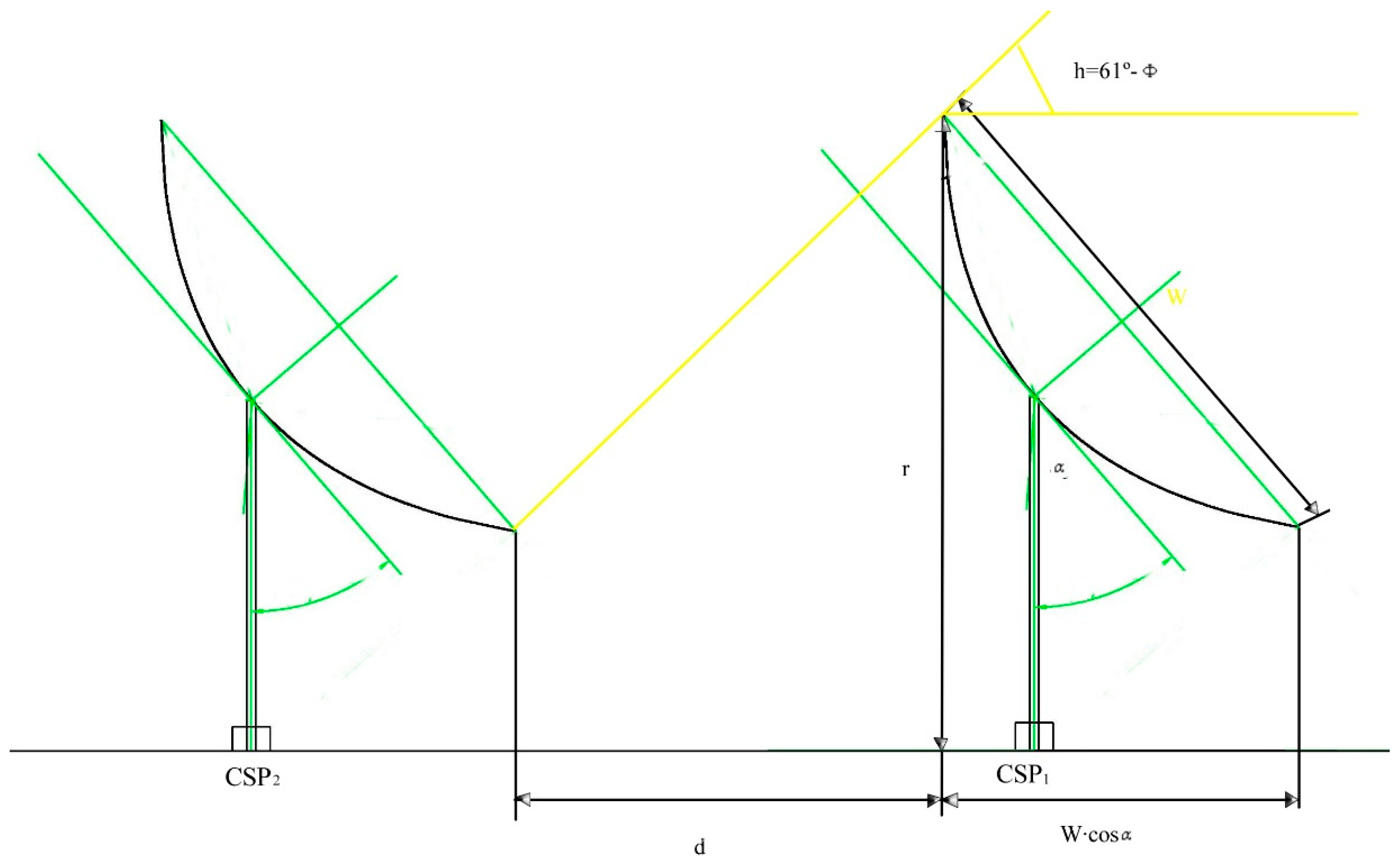
3. Standard Methods for Determining the Spacing between Collectors in PTC Facilities

3.1. Standard Method 1

It is based on the calculation of the distance (D) between the PTCs as a function of the height of the sun (h) for whom the facility was designed. Figure 3 shows the geometry to derive Equation (4):
D = d + d = W · c o s α t g   h + W   s i n   α
D = W · ( c o s α t g   h + s i n   α )
where W is the width of opening plane and α is the tilt angle relative to the vertical of the collector (azimuth of the panel). α is calculated to achieve sun rays perpendicular- Collector along the entire operating time of the solar plant. α is the solar tracking parameter which varies continuously all the time depending on the time, day, and location of the PTC facility.
In this way, the shadow gets a horizontal spacing D since the first line of the PTC being h > h’, see Figure 4, and so the second line must at least be placed in the PTC2h. In case the sun gets a height of h’, the shading would have a horizontal spacing D’, and the second PTC line would be positioned in PTC2h’.
Figure 4 shows the shadow geometry of the first PTC line (PTC 1) over the second PTC line (PTC 2 h).

3.2. Standard Method 2

This other standard method is used mainly in Spain, so that four hours of sunshine are ensured around midday on the winter solstice. In this way, in place of estimating the positions for a particular sun height, the latitude of the place is the necessary data for the use of this other standard method. It is obtained that the measured distance across the rows (d) of the PTCs of height W’ is shown at Equation (5) (Figure 5) [27].
d W · k
where k is the zero-dimensional factor, which varies according to the latitude of the place
k = 1 tg   ( 61 ° Φ )
and Φ as latitude in (°).
The spacing achieved (d) should be added to the horizontal length collector spacing at an inclination angle (α), W·sin α, as reported on Equation (7) [28].
D = d + d = W tg   ( 61 ° Φ ) + W sin   α = W ( cos α tg   ( 61 ° Φ ) + sin   α )

4. Proposed Method

The proposed method provides for the estimation of the accurate shadowing projection of PTCs for every solar hour. This process, it should be used to estimate the optimal use of area in accordance with the energy needs of PTC installations at a given location for a latitude done (Φ) based on the amount of solar gain and the inclination of the collector (α, angle relative to the horizontal PTC panel β).
In this way, the shadow projected on the ground for each PTC can be calculated using three directions: north, east, and west. For this, it is necessary to know the azimuth of the sun at the winter and summer solstices.
With the geometry and the tilt angle of the collector and using the data from the geometrical relations, shadows can be calculated for both of the corners of each PTC, and thus the surrounding polygon of the shadow path as a maximum area. Therefore, the envelope will be the exterior silhouette that forms the shadow for the period studied (see Figure 6). Thus, it is possible to calculate the minimum distance between the rows of PTCs avoid the effect of shadows in the period studied.
Figure 7 shows a flowchart of the methodology followed where from the data of the PTC field location and its dimensions and inclination, all the necessary data for the calculation of the distance between pylons without shadowing are calculated.

4.1. Solar Angle Calculation

At a specific latitude, the height of the sun depends on the hour. To establish the height of the sun-latitude relationship, basic knowledge of celestial physics is used, where the planet Earth is located in the centre (Figure 8). The equatorial plane of the celestial sphere (NS) is the equatorial plane of the Earth, where the azimuth is positive when viewed from the north (A), A* = 360° − A, i.e., clockwise.
The angle of the astronomical meridian with the equatorial plane is the solar height (h), Φ is the latitude, and δ is the declination angle of the Earth. Therefore, to determine the solar height (h) at a particular time (H) at some location on Earth (latitude), for a spherical triangle, the corresponding equations of spherical trigonometry are employed logically, as presented in Figure 7.
If a spherical triangle is used, the Z point will be the origin of the coordinates. Note that the sides are the angles in radians. Therefore, in our case, the sides of the triangle are:
  • (90° − δ) ⇒ hour angle (H)
  • (90° − Φ) ⇒ the azimuth supplement (A*)
  • (90° − h) ⇒ solar height (h)
Using the law of sines to link all these variables in one system of equations, the first two sides and their angles can be replaced according to Equation (8) [28]:
( 90 ° δ ) sin ( A ) = ( 90 ° h ) sin H
sin ( 90 ° δ ) sin ( 360 ° A ) = sin ( 90 ° h ) sin H cos δ sin A = cos h sin H
In the last two fractions, the sine of the 90° and 360° angles are 1 and 0, respectively. In addition, sin (90° − v) = cos v, sin (360° − r) = −sin (r), giving the next equation:
cos δ · sin H = sin A · cos h
Using spherical trigonometry, i.e., the first law of cosines next to it (90° − δ), the consequent equation is:
sin δ = sin Φ · sin h + cos Φ · cos h · cos A
Then, in spherical trigonometry, if the first law of cosines is applied for (90° − h), the next equation can be found:
sin h = sin Φ · sin δ + cos Φ · cos δ · cos H
Thus, the value of h is obtained in terms of the variables (δ, Φ, H).
On the other hand, it is also necessary to know the measures and inclinations (β, α) of the PTC to calculate the shadow. To establish the shading end points, we must consider at first that the solar hours are used for the design of the PTC facility. The solar hours refer to the central peak hour (H0) and the hours that are equally divided backwards and forwards from this central hour. The central peak is assumed to be H0 = 0° for the Greenwich meridian, with each hour corresponds to 15 degrees, with the adding on the right of 15 degrees per hour of solar gain and the subtracting on the left of 15° per hour (with 0 assumed to be 360° to prevent values of angles as negative). e.g., in Spain, for a setting of four hours of sun, at the time of 10:00 h, there would be an H of 330°, and at 12:00 h, it is reached an H of 30° (see Figure 9 as guidance).

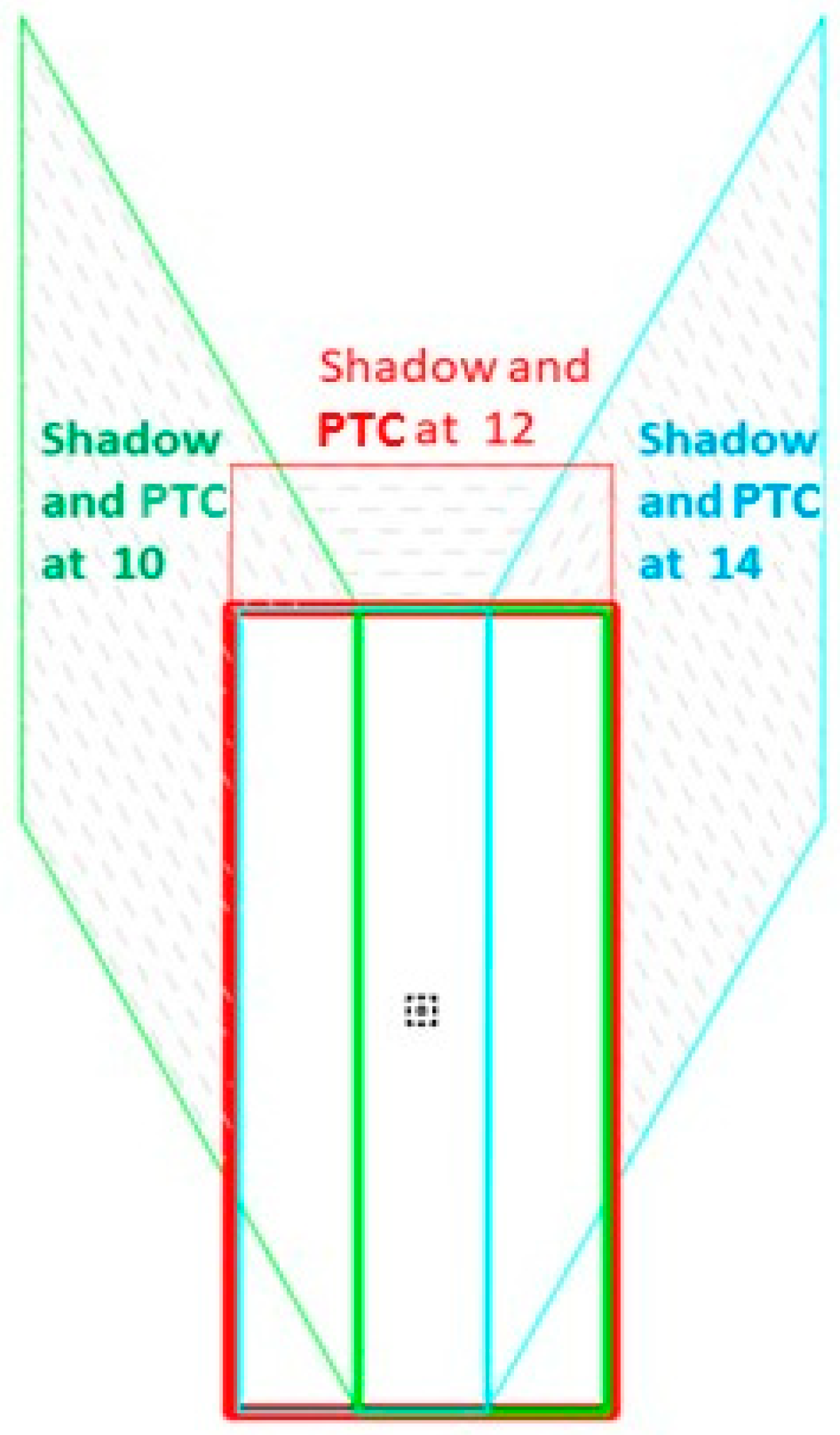
4.2. The Extent of the Shade

For the estimation of the shadow, the four corners of the concentrator are chosen. So, with known values of δ, Φ, H, and using Equation (12), it can be calculated the projected shadow (see Figure 10), where the shadow is calculated at 10, 12, and 14 h in continuous time. The outer contour of both shadows will be the envelope, these are shown in Figure 10, where the contours of full shadow at 10, 12, and 14 h have been represented.
Afterward, the distance (d) to the shading for every point is calculated based on Equation (12), linking the tilt angle of the PTC corner, the length, and the sun height.
d = W · cos α tg   h
Until now, the PTC’s corners have been projected at shadow distances (di). To plot these shading distances on the floor, polar coordinates are applied, whereby the angle Hi is the hourly angle of the point i. The critical event is the shortest day of one year, where h represents the shortest day of the solar field design. The shading envelope of a PTC is obtained, and from this envelope, the shadow projected for each whole row of the PTC assembly can be drawn so that no shadow can be cast between the rows.
The data to be computed is the spacing between the rows of PTC lines or the distance between the pylon (see Figure 11), the triangle must be solved, whose vertexes are: shadow of the first hour, shadow of the last hour (third point), and the projection of the corner of PTC. The vertex angle P is (360 − (H1 − H3)), meaning the difference in the hour angles of the other two vertexes, and the sides from point P to first point and to third point are d1 and d3, respectively. Before for h1 and h3 are calculated the values of d1 and d3. Then, it is possible to determine an effective distance of shade considering the projection angle of the sun, as shown in Equation (14) (Figure 11),
d = d · sin H = W ( cos α tg   h ) · sin H
where the distance between the pylon can be obtained depending on the dimension’s collector, the angle from the vertical of the collector, the solar hour angle, and height, as shown in the following Equation (16). In short, the distance depends the dimensions of the collector and the location of the solar field.
Distance   between   the   pylon = d + d = W ( cos α · sin H tg   h ) + W sin α
Distance   between   the   pylon = W ( sin α + cos α · sin H tg   h )
The hour angle (H) corresponds to the position of the observer with respect to the sun and the azimuth angle (A) is based on the position of the observer with respect to the north. Then, by using Equation (12), shadows at sunrise are calculated, Ortho, h = 0°, that is, sin h = 0; where for the equations, the angles are used in radians, whereas the solutions are expressed as degrees (°) to make it more user friendly (Equation (17)).
0 = tg Φ·tg δ + cos H
The result of the calculations in HORTHO° and HSUNSET°.
Considering the opening plane size as standard one, W = 5.760 m and focal distance f = 1.710 m for the distance calculation. Known W and f, it is possible the calculation of the distance of the vertex of the collector perpendicular to the aperture plane according to Equation (18):
z = ( W 2 ) 2 4 f

5. Results and Discussion

5.1. Case Study: Results

The case study will be the most unfavourable day, i.e., on December 22, the winter solstice. The shadow projected by each PTC was estimated, allowing to determine the minimum distance of the next row of PTC. The first case of study was situated in the southern of Spain, CIEMAT-PSA research centre (latitude 37.091° N; longitude 2.355° W). The data used were declination δ = −23° 27′; latitude Φ = 37.093° N, for Equations (11) and (12). It is estimated that in this location the PTCs do not reach adequate temperature to start working until two hours after sunrise. Therefore, in this case, the shadows will be calculated for the period of time in which the installation is in service. That is, from 10 to 14 h.
HORTHO and HSUNSET are calculated using Equation (17), obtaining HORTHO = 289.09° and HSUNSET = 70.91°.
Table 1 shows the results obtained for each shadow of the three points (first and third) as shown in Figure 9 and Figure 10. These outputs are considered to be valid for every point in time at which the shading distance was calculated. The known angles H1 = 330°; H3 = 30°, angles (h1, h3), and distances d (d1 y d3) are computed, considering the dimensions of a standard PTC of the commonly used Eurotrough model [29] (the aperture plane size W = 5.760 m and focal distance f = 1.710 m) for the calculation of the distance of the vertex of the collector perpendicular to the aperture plane according to Equation (18), resulting in that z = 1.212 m.
As can be observed in the results presented in Table 1, the distance calculated between PTC pylons shows a perfect symmetry throughout the day with respect to the moon, as was expected. This fact proves that a first and essential requirement to check the validity of the proposed model is accomplished.

5.2. Extension of the Case Study to Worldwide

The proposed model has been calculated in several key locations for PTC facilities in the northern hemisphere, from a latitude of 14 degrees to almost 51 degrees. Table 2 summarizes the results obtained. Clearly, the distance increases with increasing latitude.
If, from the data obtained in Table 2, a simple model is established to calculate the shadow of a standard concentrator (the opening plane size W = 5.760 m and focal distance f = 1.710 m), where S is the calculated shadow and Lat is the northern latitude, the following models are obtained:
The Linear Estimation:
S = 0.0796 Lat + 9.9243
with R2 = 0.9769
The Polynomial Estimation:
S = 0.001 Lat2 + 0.0121 Lat + 10.9
with R2 = 0.9984
If the solutions that would be obtained with each model are represented. Figure 12 is obtained, where, the area marked in green, which is to say between 20 and 45 degrees north latitude, there is scarce difference between both models. Outside this area, the linear model underestimates the magnitude of the shadow and therefore its use would not be advisable. For example, at 14 degrees north latitude, the linear model underestimates the shadow by 25 cm, while the polynomial model underestimates it by less than 3 cm. In short, the results suggest the use of the polynomial model obtained for the calculation of the shadows since it offers very good results as it has an R2 greater than 99.8%.
If the maximum value obtained for the distance between the PTC pylons is noted, a separation of around 11 to 14 m must be selected for the layout of the solar field during the design phase. This would involve a significantly lower land occupation (around 50% lower) compared to the total area to be covered if the thumb rule (of four times the aperture area) is considered. Consequently, the model presented is this work is a very useful tool for CSP plant designer because it is easy to apply, and the investment costs are significantly reduced thanks to the reduction in the land occupation for the solar field.

6. Conclusions

In this work, a new methodology has been proposed for calculating the shadows of parabolic-trough solar collectors, PTC, depending on the geographical latitude of the CSP plant location. The latitude and the standard dimensions of a standard PTC has been considered. In addition, the distance between PTC suggested was calculated by estimating that the start-up of the plant is done around two hours after the sunrise. Since the model developed, although not complex but needs quite a lot of calculations, an approximate model has been calculated for this type of standard CSP, obtaining a linear with R2 of 97.69% and a polynomial model with R2 of 99.8%. Both run well within the range of 20 to 45 degrees latitude, but outside this zone, the polynomial model works best. In short, it is proposed to use the polynomial model obtained. Furthermore, this work opens new perspectives for the calculation of shadows in CSPs plants since the methodology developed in this work can be used to establish simple shadow calculation models when the dimensions of the PTC are different from the one used in this work (or even if other type of CSP collectors are studied) or when the operating times of the installation are different.

Author Contributions

N.N., A.F.-G. and F.M.-A. conceived, designed the research and wrote the manuscript. All authors have read and agreed to the published version of the manuscript.

Funding

No external funding was received for this research.

Acknowledgments

The authors would like to thank to the CIAIMBITAL (University of Almeria, CeiA3) for its support. The manuscript was funded by I+D+I Project UAL18-TIC-A025-A, University of Almeria, the Ministry of Economy, Knowledge, Business and University and the European Regional Development Fund (FEDER).

Conflicts of Interest

The authors declare no conflict of interest. The funders had no role in the design of the study; in the collection, analyses, or interpretation of data; in the writing of the manuscript; or in the decision to publish the results.

References

  1. Baños, R.; Manzano-Agugliaro, F.; Montoya, F.; Gil, C.; Alcayde, A.; Gómez, J. Optimization methods applied to renewable and sustainable energy: A review. Renew. Sustain. Energy Rev. 2011, 15, 1753–1766. [Google Scholar] [CrossRef]
  2. Schaeffer, M.; Hare, W.; Rahmstorf, S.; Vermeer, M. Long-term sea-level rise implied by 1.5 °C and 2 °C warming levels. Nat. Clim. Chang. 2012, 2, 867–870. [Google Scholar] [CrossRef]
  3. Meyers, S.; Schmitt, B.; Vajen, K. The future of low carbon industrial process heat: A comparison between solar thermal and heat pumps. Sol. Energy 2018, 173, 893–904. [Google Scholar] [CrossRef]
  4. Miao, C.; Fang, D.; Sun, L.; Luo, Q.; Yu, Q. Driving effect of technology innovation on energy utilization efficiency in strategic emerging industries. J. Clean. Prod. 2018, 170, 1177–1184. [Google Scholar] [CrossRef]
  5. Alfaris, F.; Juaidi, A.; Manzano-Agugliaro, F. Intelligent homes’ technologies to optimize the energy performance for the net zero energy home. Energy Build. 2017, 153, 262–274. [Google Scholar] [CrossRef]
  6. Massidda, L.; Marrocu, M. Decoupling Weather Influence from User Habits for an Optimal Electric Load Forecast System. Energies 2017, 10, 2171. [Google Scholar] [CrossRef] [Green Version]
  7. Massidda, L.; Marrocu, M. Use of Multilinear Adaptive Regression Splines and numerical weather prediction to forecast the power output of a PV plant in Borkum, Germany. Sol. Energy 2017, 146, 141–149. [Google Scholar] [CrossRef]
  8. Islam, T.; Huda, N.; Abdullah, A.; Saidur, R. A comprehensive review of state-of-the-art concentrating solar power (CSP) technologies: Current status and research trends. Renew. Sustain. Energy Rev. 2018, 91, 987–1018. [Google Scholar] [CrossRef]
  9. Hernandez-Escobedo, Q.; Rodriguez-Garcia, E.; Saldaña-Flores, R.; Fernández-García, A.; Manzano-Agugliaro, F. Solar energy resource assessment in Mexican states along the Gulf of Mexico. Renew. Sustain. Energy Rev. 2015, 43, 216–238. [Google Scholar] [CrossRef]
  10. Sansaniwal, S.K.; Sharma, V.; Mathur, J. Energy and exergy analyses of various typical solar energy applications: A comprehensive review. Renew. Sustain. Energy Rev. 2018, 82, 1576–1601. [Google Scholar] [CrossRef]
  11. Sengupta, M.; Xie, Y.; Lopez, A.; Habte, A.; Maclaurin, G.; Shelby, J. The National Solar Radiation Data Base (NSRDB). Renew. Sustain. Energy Rev. 2018, 89, 51–60. [Google Scholar] [CrossRef]
  12. Manzano-Agugliaro, F.; Alcayde, A.; Montoya, F.; Zapata-Sierra, A.J.; Gil, C. Scientific production of renewable energies worldwide: An overview. Renew. Sustain. Energy Rev. 2013, 18, 134–143. [Google Scholar] [CrossRef]
  13. Cruz-Peragón, F.; Palomar, J.; Casanova, P.; Dorado, M.; Manzano-Agugliaro, F. Characterization of solar flat plate collectors. Renew. Sustain. Energy Rev. 2012, 16, 1709–1720. [Google Scholar] [CrossRef]
  14. Behar, O.; Khellaf, A.; Mohammedi, K. A review of studies on central receiver solar thermal power plants. Renew. Sustain. Energy Rev. 2013, 23, 12–39. [Google Scholar] [CrossRef]
  15. Fernández-García, A.; Rojas, E.; Pérez, M.; Silva, R.; Hernandez-Escobedo, Q.; Manzano-Agugliaro, F.; Pérez-García, M. A parabolic-trough collector for cleaner industrial process heat. J. Clean. Prod. 2015, 89, 272–285. [Google Scholar] [CrossRef]
  16. Sutter, F.; Fernández-García, A.; Wette, J.; Reche-Navarro, T.J.; Martínez-Arcos, L. Acceptance criteria for accelerated aging testing of silvered-glass mirrors for concentrated solar power technologies. Sol. Energy Mater. Sol. Cells 2019, 193, 361–371. [Google Scholar] [CrossRef]
  17. Kasaeian, A.; Nouri, G.; Ranjbaran, P.; Wen, D. Solar collectors and photovoltaics as combined heat and power systems: A critical review. Energy Convers. Manag. 2018, 156, 688–705. [Google Scholar] [CrossRef] [Green Version]
  18. García-Segura, A.; Fernández-García, A.; Ariza, M.; Sutter, F.; Diamantino, T.; Martínez-Arcos, L.; Reche-Navarro, T.; Valenzuela, L. Influence of gaseous pollutants and their synergistic effects on the aging of reflector materials for concentrating solar thermal technologies. Sol. Energy Mater. Sol. Cells 2019, 200, 109955. [Google Scholar] [CrossRef] [Green Version]
  19. Jin, J.; Ling, Y.; Hao, Y. Similarity analysis of parabolic-trough solar collectors. Appl. Energy 2017, 204, 958–965. [Google Scholar] [CrossRef]
  20. Bellos, E.; Tzivanidis, C. Enhancing the performance of a parabolic trough collector with combined thermal and optical techniques. Appl. Therm. Eng. 2020, 164, 114496. [Google Scholar] [CrossRef]
  21. Asociación Española para la Promoción de la Industria Termosolar. Informe de Transición del sector Eléctrico Horizonte 2030. 2018. Available online: http://www.protermosolar.com (accessed on 10 December 2019).
  22. Bellos, E.; Tzivanidis, C. Alternative designs of parabolic trough solar collectors. Prog. Energy Combust. Sci. 2019, 71, 81–117. [Google Scholar] [CrossRef]
  23. Bellos, E.; Tzivanidis, C. Investigation of a nanofluid-based concentrating thermal photovoltaic with a parabolic reflector. Energy Convers. Manag. 2019, 180, 171–182. [Google Scholar] [CrossRef]
  24. Fernández-García, A.; Juaidi, A.; Sutter, F.; Martínez-Arcos, L.; Manzano-Agugliaro, F. Solar Reflector Materials Degradation Due to the Sand Deposited on the Backside Protective Paints. Energies 2018, 11, 808. [Google Scholar] [CrossRef] [Green Version]
  25. Sánchez-Lozano, J.; García-Cascales, M.; Lamata, M. Evaluation of suitable locations for the installation of solar thermoelectric power plants. Comput. Ind. Eng. 2015, 87, 343–355. [Google Scholar] [CrossRef]
  26. Kalogirou, S. Solar Energy Engineering, Processes and Systems; Academic Press: New York, NY, USA, 2014; 819p, ISBN 978-0-12-397270-5. [Google Scholar]
  27. IDEA (Instituto para la Diversificación y Ahorro de la Energía). Anexo III. Cálculo de pérdidas de radiación solar por sombras. In Instalaciones de Energía Solar Térmica, Pliego de Condiciones Técnicas de Instalaciones de Baja Temperatura; IDEA: Madrid, Spain, 2011; pp. 40–44. [Google Scholar]
  28. Castellano, N.N.; Parra, J.A.G.; Valls-Guirado, J.; Manzano-Agugliaro, F. Optimal displacement of photovoltaic array’s rows using a novel shading model. Appl. Energy 2015, 144, 1–9. [Google Scholar] [CrossRef]
  29. Fernández-García, A.; Zarza, E.; Valenzuela, L.; Perez, M. Parabolic-trough solar collectors and their applications. Renew. Sustain. Energy Rev. 2010, 14, 1695–1721. [Google Scholar] [CrossRef]
Figure 1. Scheme of working of a PTC facility. (1) Reflector; (2) Absorber tube; (3) Structure; (4) Solar Field Piping.
Symmetry 12 00278 g001
Figure 2. Geometry on a PTC for the sun’s rays (section view).
Symmetry 12 00278 g002
Figure 3. Geometry on a PTC for the sun’s rays (frontal view).
Symmetry 12 00278 g003
Figure 4. Row alignment minimum PTC depending on the solar altitude (Standard Method 1).
Symmetry 12 00278 g004
Figure 5. Minimum PTC row alignment as solar altitude function (standard method 2).
Symmetry 12 00278 g005
Figure 6. Proposed method: isometric view of PTC. (A) Shadowing at 10 a.m.; (B) Shadowing at 12 a.m.
Symmetry 12 00278 g006
Figure 7. Flowchart of the methodology for the calculation of the distance of a PTC row.
Symmetry 12 00278 g007
Figure 8. Spherical triangle model for the estimation of the sun’s shadow at a specific latitude.
Symmetry 12 00278 g008
Figure 9. Shadows. (a) Shadow at 10:00, (b) shadow at 12:00; and (c) Shadow at 14:00.
Symmetry 12 00278 g009
Figure 10. Range of the total projection of the collector’s shadow.
Symmetry 12 00278 g010
Figure 11. Diagram of d‴ calculation polygons.
Symmetry 12 00278 g011
Figure 12. Different models obtained for the calculation of shadows in depending on the latitude.
Symmetry 12 00278 g012
Table 1. Calculations for every shadow of the three points at south of Spain on 22 December 2019 (latitude 37.091° N).
Solar HourTime Angle (° (H)Elevation or Solar Height (°) (h)Flat Tilt Opening (°) (α)Distance between Pylons (m) d‴ + d′ = W (sinα + cosα (sin H/tg h))
10:00:00330.0000.41640.6668.847
12:00:00300.0000.50089.9995.760
14:00:00270.0000.58340.6658.847
Table 2. Calculations according to the proposed modelling the main PTC facilities in the northern hemisphere.
CountryEmplacementLatitude (° N)Solar Hour (2 h after Sunrise)Calculated Shadow Distance d‴ + d′ = W (sinα + cosα (sin H/tg h)) (m)
ThailandKanchanaburi 14.0228:25:0711.294
USAKailua-Kona (Hawai)19.6398:35:4311.546
UEAMedinat Zayed (Abu Dabi)23.6608:43:0011.749
USAIndiantown (Florida)27.0278:51:0711.957
AlgeriaHassiR’mel32.9289:05:0712.407
MoroccoAin Beni Mathar (Oujda)34.0889:08:0012.508
USAMojave Desert (California)35.0319:10:0012.593
SpainAlmeria 37.0519:16:2512.787
ItalyMassa Martana42.77610:08:5913.374
CanadaKingsey Falls (Québec)45.8609:46:0013.699
GermanyJülich50.92210:08:5914.147

